

Abstract
Laser-induced fluorescence measurements of singly-charged xenon ion velocities in Hall thrusters typically target metastable states due to lack of available laser technology for exciting the ground state. The measured velocity distribution of these metastable ions are assumed to reflect the ground state ion behavior. However, this assumption has not been experimentally verified. To investigate the accuracy of this assumption, a recently developed xenon ion (Xe II) collisional-radiative model is combined with a 1D fluid model for ions, using plasma parameters from higher fidelity simulations of each thruster, to calculate the metastable and ground state ion velocities as a function of position along the channel centerline. For the HERMeS and SPT-100 thruster channel centerlines, differences up to 0.5 km s−1 were observed between the metastable and ground state ion velocities. For the HERMeS thruster, the difference between the metastable and ground state velocities is less than 150 m s−1 within one channel length of the channel exit, but increases thereafter due to charge exchange (CEX) that reduces the mean velocity of the ground state ions. While both the ground state ions and metastable state ions experience the same acceleration by the electric field, these small velocity differences arise because ionization and CEX directly into these states from the slower neutral ground state can reduce their mean velocities by different amounts. Therefore, the velocity discrepancy may be larger for thrusters with lower propellant utilization efficiency and higher neutral density. For example, differences up to 1.7 km s−1 were calculated on the HET-P70 thruster channel centerline. Note that although the creation of slow ions can influence the mean velocity, the most probable velocity should be unaffected by these processes.

Original content from this work may be used under the terms of the Creative Commons Attribution 4.0 license. Any further distribution of this work must maintain attribution to the author(s) and the title of the work, journal citation and DOI.
1. Introduction
For Hall thruster development and testing, it is important to thoroughly characterize and understand the plasma behavior such as ion velocities in the thruster channel and plume. Laser-induced fluorescence (LIF) is a minimally-invasive plasma diagnostic tool that is used to measure spatially-resolved and sometimes temporally-resolved ion velocity distribution functions (IVDFs). These measurements can validate or inform Hall thruster models and estimates of facility effects and on-orbit behavior [1–3]. Measurements of ion dynamics are also useful for improving understanding of the physics involved in Hall thrusters and observed phenomena such as anomalous electron transport [4–10]. Since LIF is a well established diagnostic used throughout the electric propulsion community, it is important to be aware of the assumptions involved and to investigate those assumptions when possible [11].
In LIF, a laser is directed into a plasma. Ions moving along the beam direction see the Doppler shifted laser frequency. If their velocity is such that the photon energy matches the energy of a bound electron transition, they can absorb the photon, exciting them to a higher energy level which then spontaneously decays and emits a measurable fluorescent signal. By sweeping the laser over a range of wavelengths, ions moving at different velocities are probed, and the Doppler shift of the excited ions is calculated in constructing the IVDF.
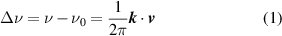
where is the Doppler shift from the recorded frequency in the lab frame, ν, and the unshifted frequency in the ion's frame, ν0. Writing this in terms of wavelength as is done in LIF experiments, the velocity parallel to the wave vector v , vk is given by

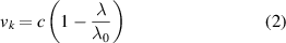
where λ0 is the central wavelength of the transition in the ion's frame, and λ is the laser photon wavelength in the lab frame.
There are two common transition schemes shown in figure 1 for xenon ions used in LIF, both starting from metastable levels. Metastable states are chosen since they have a relatively large population to be excited, and thus higher signal to noise ratio. In the first non-resonant scheme [12], the ions at metastable level are excited by the laser at 605.28 nm to . This upper level de-excites to , resulting in fluorescence at 529.36 nm. In the second [13], now more commonly used scheme, ions at metastable level are excited by the laser at 834.95 nm to . Then, de-excitation occurs to , resulting in fluorescence at 542.06 nm. (The wavelengths listed here are in-vacuum values.) This scheme is possible with commercial diode lasers. The first scheme could be achieved with dye lasers. In both transition schemes, the ground state (g.s.) ion is not directly probed. However, it is commonly assumed that the dynamics of the metastable ions represent the dynamics of the ground state ions. This assumption has not been verified since practical tunable laser technologies are not available for exciting ions out of the ground state and thus directly measuring the g.s. IVDF.
![$5p^4(^3P_2)5d^2[3]_{7/2}$](https://content.cld.iop.org/journals/0963-0252/32/1/015009/revision2/psstacb00bieqn2.gif)
![$5p^4(^3P_2)6p^2[2]^o_{5/2}$](https://content.cld.iop.org/journals/0963-0252/32/1/015009/revision2/psstacb00bieqn3.gif)
![$5p^4(^3P_2)6s^2[2]_{5/2}$](https://content.cld.iop.org/journals/0963-0252/32/1/015009/revision2/psstacb00bieqn4.gif)
![$5p^4(^3P_2)5d^2[4]_{7/2}$](https://content.cld.iop.org/journals/0963-0252/32/1/015009/revision2/psstacb00bieqn5.gif)
![$5p^4(^3P_2)6p^2[3]^o_{5/2}$](https://content.cld.iop.org/journals/0963-0252/32/1/015009/revision2/psstacb00bieqn6.gif)
![$5p^4(^3P_2)6s^2[2]_{3/2}$](https://content.cld.iop.org/journals/0963-0252/32/1/015009/revision2/psstacb00bieqn7.gif)

Figure 1. Partial energy diagrams of LIF transition schemes for singly ionized xenon.
Download figure:
Standard image High-resolution imageTherefore, the objective of this paper is to assess the accuracy of using the metastable ion state velocity as representative of the ground state ion velocity. The Xe II collisional-radiative (CR) model recently developed by JPL [14, 15] is augmented with one-dimensional ion continuity and momentum equations in order to calculate the metastable ion velocity for a given set of plasma parameters, and therefore answer this question. The approach is to choose a thruster with spatially resolved plasma parameters known from validated discharge simulations. Then, using these parameters as inputs to the CR model, we calculate the populating and depopulating rates for each process and energy level included in the model. Using the discretized form of the conservative fluid equations, the velocity and density positional profiles of each energy level included in the model are calculated starting from an initial position where the ion velocity is near zero, integrating along the direction of ion motion. Finally, the ion ground state velocity profile is compared to the velocity profiles of the metastable ions used in LIF. The following sections will discuss this approach and present key results regarding the extent to which the assumption is accurate.
2. Approach
2.1. Hall thruster regimes
We briefly discuss common terminology for Hall thruster geometry and regimes that are referenced in the following sections. We will also discuss the sources of the plasma parameters of the Hall thruster test cases considered. Figure 2 shows a Hall thruster with a centrally mounted cathode which emits electrons. Ions are created inside the channel as neutral gas is injected at the anode in the back of the channel and is ionized by electrons. The location where most ionization occurs is defined as the ionization region. Note that the ionization region may overlap with the acceleration region [13]. Then, ions are accelerated near the channel exit, where they are accessible to LIF diagnostics. The focus of this paper is this acceleration region of ions along the channel centerline.

Figure 2. Hall thruster regions.
Download figure:
Standard image High-resolution imageSeveral thruster test cases are used, including NASA's 12.5 kW HERMeS thruster [16]. Plasma parameters for this thruster are taken from outputs from Hall2De, an experimentally validated Hall thruster code [2, 6–8, 17]. The second test case is the SPT-100 thruster using published simulation outputs [18]. A laboratory thruster, HET-P70, is also considered, with some channel centerline parameters tabulated in Zhu et al [19]. The remaining HET-P70 input parameter profiles are interpolated to have a similar shape as the HERMeS input parameter profiles. These multiple test cases are included to assess the accuracy of the assumption for a range of plasma input parameters.
2.2. Fluid equations
In order to calculate the velocity and density of an excited state in a simple, computationally inexpensive way, we take a fluid approach to the problem. The fluid equations can be derived starting from the 1D Boltzmann equation
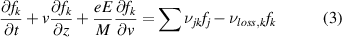
where is the velocity distribution of state k, and νjk and are the source and sink frequencies, respectively. The source and sink frequencies can be calculated from the Xe II CR model and are explained in the next section. The fluid continuity equation can be derived by taking the zeroth moment of the Boltzmann equation, and the momentum equation is derived by taking the first moment of the Boltzmann equation. Assuming steady-state and no pressure term (i.e. zero ion temperature), the resulting fluid equations are


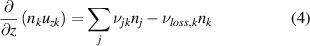
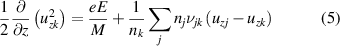
where E is the axial electric field, uzk is the axial velocity of state k, and nk is the population density of state k. We note that this is the conservative form of the momentum equation, so that depopulation events do not affect the velocity of an excited state.
2.3. Xe II CR model
A CR model for singly-charged xenon ions has recently been developed by JPL and compared with experiments [14, 15]. The model was based closely on a CR model for Xe II published by Zhu et al [19], which was made possible by theoretical electron-impact excitation cross sections and spontaneous transition rates published by Wang et al [20]. This CR model can be used to calculate the source and sink frequencies for each xenon ion excited state, which when combined with the fluid equations, can be used to calculate the velocity of the metastable state ions used in LIF. The structure of this CR model is more thoroughly discussed in Chaplin et al [14], with the relevant information and equations given here. The model assumes the plasma is optically thin. Although transitions to the ground state will be significantly absorbed, the transition rate to the ground state from the main non-metastable state explored in this paper is only about one tenth of the total decay rate to other excited states. We calculated the optical thickness of the plasma for the two dominant decay paths at the middle of the acceleration region in HERMeS to be 1 using equation (15) of [14]. Therefore, we expect minimal re-absorption.

In the original 0D version of the CR model, to calculate the population density of an ion excited to some state k, nk , the steady-state rate equation is solved by summing the populating and depopulating processes rates to or from other states j, given in equation (6):
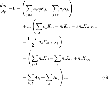
The Xe II model includes the 6s, 5d, and 6p states, with a total of 57 excited states, k. Here, in addition to the subscripts k and j, subscript g refers to the near-ground states of singly-charged xenon ion, and n refers to the ground state of neutral xenon. The rate coefficient, K, for transitions between levels indicated by the subscript is calculated by averaging the cross-section of a transition over the electron velocity distribution f(v), assuming f(v) is a Maxwellian. A is the Einstein coefficient or spontaneous emission rate between the levels also indicated by the subscript. α is defined as the ratio of singly-charged ion density, , to electron density, ne .

The populating methods summarized in equation (6) include e- impact excitation and de-excitation from lower and higher states, spontaneous emission from upper states, e- impact excitation from the near-ground states, and e- and ion impact ionization from the neutral xenon ground state. Depopulating methods include e- impact excitation and de-excitation to higher and lower states, e- impact de-excitation to the near ground states, ionization, and spontaneous emission to lower states, including the near ground states. The expressions for populating and depopulating rates are incorporated in the equations for source and sink frequency terms.
The cross-sections for electron impact excitation are exclusively taken from Wang et al [20] which were calculated using the Dirac-B-spline R-matrix (DBSR) method. The electron impact de-excitation cross sections are calculated using detailed balance [21]. For electron impact ionization-excitation, the cross sections for transitions from the Xe I ground state to eight Xe II 6p levels were measured by Chiu et al [22]. The cross-sections for transitions to the remaining Xe II 6p, 5d, and 6s levels are estimated based on averages and analogies of the known cross-sections. Similarly, the ion-impact excitation cross-sections from the Xe I ground state to the same Xe II 6p levels are given by [22]. The measurements are only at 300 eV for Xe+ impacts and 600 eV for Xe2+ impacts, and the cross-sections are assumed to be independent of energy. These cross-sections are less important than electron-impact excitation cross-sections except at very low electron temperature [23], so the neglect of their weak energy dependence is not expected to significantly increase the uncertainty in our results. Finally, for spontaneous emission rates, experimental data from the NIST database [24] was used when possible. However, the majority of transitions for Xe II were the theoretical DBSR results from Wang et al [20]. Since no DBSR calculations of ionization cross-sections out of excited states were available, the Deutsch-Märk formalism [25] was used to estimate these cross sections.
2.4. Overall computational approach
Given this background, the computational approach for calculating the density and velocity axial profiles of excited states k is to first obtain thruster parameters either from simulations or other published data. Then using these parameters as inputs to the Xe II CR model, calculate the source and sink collision rates (νjk and ):


where Ajk in equation (7) is only finite when j > k. The sum over j in equations (4) and (5) encompasses other xenon ion states including the ground and near ground states and the neutral xenon ground state. The source collision rate specifically from the neutral xenon ground state which is included in could be written separately as

which includes ion impact ionization-excitation (term in parentheses) and electron impact ionization-excitation from the neutral xenon ground state.
Then, these rates and the thruster parameters are interpolated to achieve a smaller step size which are input to the discretized conservative form of the fluid equations. The smaller step size is needed to reduce the local error and avoid unphysical solutions. Using the forward Euler method, the discretized fluid equations are arranged to solve for the velocity and density profiles of an excited state:
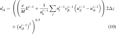
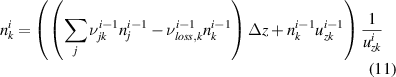
where i is the index of the axial mesh node, and is the mesh spacing or step size.

The overall computational approach is shown in figure 3. The discretized momentum equation for a state k requires the density and velocity of other states j that are either excited or de-excited to state k. Therefore, a set of fluid equations is required to be solved at each step. In the original CR model, there are 57 energy levels. However, to save computational time, only the 39 energy levels that are coupled to the metastable states of interest are included in the calculation.

Figure 3. Flowchart of the computational approach.
Download figure:
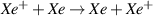
Standard image High-resolution imageAlso, to ensure that the differences calculated between the metastable ion velocities and the ground state ion velocity are due to effects that exist in the thruster, rather than differences in the terms included in the momentum equation in our simple 1D model versus those included in the codes from which we extract plasma parameters or unrealistic assumptions we used to fill in missing data, we calculate the ground state ion velocity for each thruster. In this calculation, we account for the charge exchange (CEX) reaction , where both the neutral atom and the ion are in the ground state. CEX reactions involving metastable ions are not included in the calculation of the excited state velocities because it is expected this will have a small effect on the calculated velocities and the cross section data for these processes is not available. To calculate the ground state ion velocity, we use a modified version of the momentum equation used to calculate the metastable ion velocities shown in equation (5), where state k is the ion ground state and state j is the neutral ground state. Since both the Hall2De and Panelli et al codes neglect stepwise ionization, we also only consider direct ionization. Accounting for CEX, the momentum equation becomes
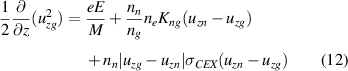
where uzg is the ion ground state velocity and uzn is the neutral ground state velocity. The CEX cross section σCEX is approximated by

where E is the collision energy, expressed in eV [26]. Throughout the calculations, a value of 250 m s−1 is used for uzn , as justified by [27]. As before, this momentum equation is discretized, and arranged to solve for the ground state ion velocity profile using the forward Euler method. By using the calculated ion ground state velocity, any differences that remain between the calculated metastable ion velocities and the ground state ion velocity must be due to real effects in the thrusters.

3. Results
In this paper, the channel centerlines of three thruster test cases (HERMeS, SPT-100, and HET-P70) are considered when assessing the assumption that the metastable state ion velocities reflect the ground state ion velocities. In each case, we will present the calculated metastable ion velocity profiles for each transition scheme. We will also present the calculated velocity profiles for a non-metastable energy level, , which is primarily populated by e- excitation from the ground state and should therefore track the ground state ion velocity well. This more simple case will serve as a proof of concept for the computational method before drawing conclusions about the metastable states which are populated by multiple processes such as e- excitation from the ground state, spontaneous emission from higher states, e- impact de-excitation from higher states, and e- ionization from the neutral xenon (Xe I) ground state. The normalized populating processes for metastable level and non-metastable level along the HERMeS channel centerline are shown in figure 4. Throughout this paper, the axial position, z, is normalized to the channel length, L. For the non-metastable level , the normalized contribution from e- excitation from the ground state is almost one, with a small contribution from spontaneous emission from higher states. Some processes were not included in the cross-section data set and thus do not appear since they were expected to have only a small influence on radiating 6p levels, which are the main focus of the CR model. For example, electron-impact excitation from other xenon ion excited states into 5d states is not included in the model, and thus this process does not appear in figure 4. While electron-impact ionization from the neutral xenon ground state is included for some 5d levels, it is not included for ionization to level since this level decays primarily into 6p levels, and the measured ionization-excitation cross-sections for the 6p levels include cascade contributions. Since the primary goal of the CR model was to accurately estimate the population of the 6p levels, this process was excluded to avoid double-counting ionization-excitations that ultimately lead to population of a 6p level.
![$5p^4(^1D_2)5d^2[2]_{5/2}$](https://content.cld.iop.org/journals/0963-0252/32/1/015009/revision2/psstacb00bieqn17.gif)
![$5p^4(^3P_2)5d^2[4]_{7/2}$](https://content.cld.iop.org/journals/0963-0252/32/1/015009/revision2/psstacb00bieqn18.gif)
![$5p^4(^1D_2)5d^2[2]_{5/2}$](https://content.cld.iop.org/journals/0963-0252/32/1/015009/revision2/psstacb00bieqn19.gif)
![$5p^4(^1D_2)5d^2[2]_{5/2}$](https://content.cld.iop.org/journals/0963-0252/32/1/015009/revision2/psstacb00bieqn20.gif)
![$5p^4(^1D_2)5d^2[2]_{5/2}$](https://content.cld.iop.org/journals/0963-0252/32/1/015009/revision2/psstacb00bieqn21.gif)

Figure 4. Normalized populating process rates for metastable level (left) and non-metastable level (right) along the HERMeS channel centerline.
![$5p^4(^3P_2)5d^2[4]_{7/2}$](https://content.cld.iop.org/journals/0963-0252/32/1/015009/revision2/psstacb00bieqn22.gif)
![$5p^4(^1D_2)5d^2[2]_{5/2}$](https://content.cld.iop.org/journals/0963-0252/32/1/015009/revision2/psstacb00bieqn23.gif)
Download figure:
Standard image High-resolution image3.1. HERMeS channel centerline
For the HERMeS channel centerline case, the calculated velocities and densities of each state are compared to the ground state, indicated with a black dashed line in figure 5. The velocity singly-charged ions would experience starting from rest due to acceleration from the electric field alone is also shown. The HERMeS operating condition being simulated is a discharge voltage of 300 V, discharge current of 20.83 A, and nominal magnetic field. This was chosen largely because the full power operating condition at 600 V and 20.83 A has large-amplitude discharge current and ion velocity oscillations and thus is not a good test case for a steady-state calculation.

Figure 5. Velocity (left) and density (right) profiles of each metastable level (blue and red) and non-metastable level (green) along HERMeS channel centerline.
Download figure:
Standard image High-resolution imageFrom this plot, it appears that non-metastable level ion velocity overlays the ground state ion velocity fairly well, as was expected for this simple case. The density profile of the ground state and non-metastable level ions decrease along the z-axis. The ground state density is from the Hall2De simulation and decreases because of the beam divergence included in the simulation. The non-metastable level ion population density decreases because of loss through spontaneous emission. The metastable state densities, however, remain relatively constant after about since our 1D calculation does not account for beam divergence. Also, spontaneous emission is forbidden from metastable states, and there is less energy available for collisional loss processes downstream. The remainder of this section will examine the differences between the calculated excited states' velocities and the ground state ion velocity and offer explanations for these differences.
![$5p^4(^1D_2)5d^2[2]_{5/2}$](https://content.cld.iop.org/journals/0963-0252/32/1/015009/revision2/psstacb00bieqn24.gif)
![$5p^4(^1D_2)5d^2[2]_{5/2}$](https://content.cld.iop.org/journals/0963-0252/32/1/015009/revision2/psstacb00bieqn25.gif)

Starting with non-metastable level , the difference between the excited state and the ground state is plotted with the momentum acceleration terms in figure 6. The momentum equation terms are , the acceleration due to the electric field, and , the acceleration due to the sum of populating processes. It appears that there is generally good agreement with the ground state ion velocity, with the excited state velocity up to only 30 m s−1 higher than the ground state ion velocity after the channel exit where the acceleration region is located. Beyond the acceleration region, the velocity of this non-metastable level decreases with respect to the ground state ion velocity, but only becomes about 15 m s−1 slower than the ground state ion velocity in the axial region explored. The axial profile of the normalized populating rates shown in the right plot of figure 4 reveal that around , the location at which the ground state ion velocity exceeds the excited state ion velocity, spontaneous emission from higher states has a relatively larger contribution to the population of the non-metastable state. Thus, the behavior of the levels that decay into level are examined.
![$5p^4(^1D_2)5d^2[2]_{5/2}$](https://content.cld.iop.org/journals/0963-0252/32/1/015009/revision2/psstacb00bieqn27.gif)

![$5p^4(^1D_2)5d^2[2]_{5/2}$](https://content.cld.iop.org/journals/0963-0252/32/1/015009/revision2/psstacb00bieqn30.gif)

![$5p^4(^1D_2)5d^2[2]_{5/2}$](https://content.cld.iop.org/journals/0963-0252/32/1/015009/revision2/psstacb00bieqn32.gif)

Figure 6. Difference between local axial velocity uz for non-metastable level ions, uzk , and ground state ions, , along the HERMeS normalized channel axis compared to acceleration terms from the momentum equation.
![$5p^4(^1D_2)5d^2[2]_{5/2}$](https://content.cld.iop.org/journals/0963-0252/32/1/015009/revision2/psstacb00bieqn33.gif)

Download figure:
Standard image High-resolution imageThe levels that decay into non-metastable level have velocities lower than the ground state, shown in figure 7(a), and will therefore slightly lower the mean velocity of the level they spontaneously decay to. To understand why the velocity of these upper levels is lower than the ground state, we look at the populating rates of two of the upper levels. The populating processes from the ion ground state and other ion states will result in a mean velocity close to that of the ion ground state. However, populating processes from the slower neutral ground state will lower the mean velocity.
![$5p^4(^1D_2)5d^2[2]_{5/2}$](https://content.cld.iop.org/journals/0963-0252/32/1/015009/revision2/psstacb00bieqn35.gif)

Figure 7. Axial velocity of levels that decay into level (left) and populating rates of two of these upper levels (right) along the HERMeS channel centerline.
![$5p^4(^1D_2)5d^2[2]_{5/2}$](https://content.cld.iop.org/journals/0963-0252/32/1/015009/revision2/psstacb00bieqn39.gif)
Download figure:
Standard image High-resolution imageFirst, looking at level , we see in figure 7(b) that along the channel centerline beyond the channel exit, the populating rates of the electron impact processes (black, green, and magenta) decrease. This is consistent with the fact that the electron temperature decreases downstream, and thus there are fewer electrons present with energies at which the excitation cross sections are significant. However, the rate of ion impact ionization-excitation from the neutral ground state (blue) remains relatively constant. Therefore, we expect the velocity of this state will diverge from the ground state ion velocity downstream, but the deviation will not be very large given that the populating rates of electron impact excitation from the ion ground state and from other ion states remain larger than the populating rate of ion impact ionization from the neutral ground state.
![$5p^4(^1D_2)6p^2[1]^o_{3/2}$](https://content.cld.iop.org/journals/0963-0252/32/1/015009/revision2/psstacb00bieqn36.gif)
The same pattern is observed in the populating rates for level in figure 7(c). However, in this case, the rate of ion impact ionization from the neutral ground state is much closer to that of the electron impact rates, even exceeding them by the end of the computational domain. Also, the rate of electron impact ionization from the neutral ground state makes up a greater share of the total rate in the upstream region. Therefore, we expect the velocity of this level to more strongly diverge from the ground state velocity. This is consistent with the velocity of level shown in orange in figure 7(a).
![$5p^4(^1D_2)6p^2[2]^o_{3/2}$](https://content.cld.iop.org/journals/0963-0252/32/1/015009/revision2/psstacb00bieqn37.gif)
![$5p^4(^1D_2)6p^2[2]^o_{3/2}$](https://content.cld.iop.org/journals/0963-0252/32/1/015009/revision2/psstacb00bieqn38.gif)
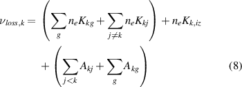
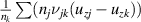
Next, to evaluate and explain the differences between the ground state ion and metastable ion velocities along the channel length, the difference between the ground state ion and metastable ion velocities are plotted with the source acceleration term in the momentum equation, , in figure 8. This source acceleration, the acceleration of state k due to populating events from other states j which have different velocities, is the second term in equation (10). Since both the ground state ions and metastable ions are accelerated by the same electric field, the source acceleration term is the key in understanding the different velocities experienced by each species. The net effect is to decelerate the bulk ion populations since the source acceleration term includes populating processes from the slower neutral ground state.
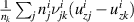

Figure 8. Difference between metastable and ground state ion velocities (blue) versus source acceleration (black) for the state (left) and state (right) along the HERMeS channel centerline.
![$5p^4(^3P_2)5d^2[4]_{7/2}$](https://content.cld.iop.org/journals/0963-0252/32/1/015009/revision2/psstacb00bieqn41.gif)
![$5p^4(^3P_2)5d^2[3]_{7/2}$](https://content.cld.iop.org/journals/0963-0252/32/1/015009/revision2/psstacb00bieqn42.gif)
Download figure:
Standard image High-resolution imageStarting with metastable state , we see that initially from , there is more acceleration for the ground state ion and so the ion velocity is initially higher than the metastable ion velocity. Then, from , there is more deceleration of the ground state ions, and thus the ground state ion velocity decreases with respect to the metastable ion velocity. From , there is more deceleration of the metastable ion velocity, and thus the ground state ion velocity increases relative to the metastable ion velocity. Finally, from , there is more deceleration of the ground state ion velocity, and thus the ground state ion velocity decreases relative to the metastable ion velocity. The vertical dashed lines correspond to the boundaries between regions mentioned above. There are two main differences between the source acceleration profiles that cause the magnitude of deceleration of the metastable state to change relative to the ground state. First, the peak deceleration of the metastable ions is lower in magnitude than that of the ground state ions. Also, the peak deceleration of the metastable ions is slightly downstream of the peak deceleration of the ground state ions. For the second metastable state, , the deceleration of that metastable state is less than the deceleration of the ground state for the entirety of the domain explored, and thus the metastable state ion velocity continuously increases with respect to the ground state ion velocity. For the remainder of this section, details of the source acceleration term are discussed only for the first metastable state, , since the same patterns will apply to the other metastable state.
![$5p^4(^3P_2)5d^2[4]_{7/2}$](https://content.cld.iop.org/journals/0963-0252/32/1/015009/revision2/psstacb00bieqn44.gif)
![$5p^4(^3P_2)5d^2[3]_{7/2}$](https://content.cld.iop.org/journals/0963-0252/32/1/015009/revision2/psstacb00bieqn49.gif)
![$5p^4(^3P_2)5d^2[4]_{7/2}$](https://content.cld.iop.org/journals/0963-0252/32/1/015009/revision2/psstacb00bieqn50.gif)
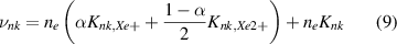
By plotting the source acceleration from each process populating the metastable ion state in figure 9, we see that electron impact ionization from the neutral ground state is the dominant reason for deceleration along the majority of the channel centerline. However, this is still smaller in magnitude than the deceleration of the ground state ions due to ionization from the neutral ground state and CEX. The magnitude of deceleration of state k is determined by the cross-sections of each transition populating that state, the energy of the electrons, and the population density of state k. In this case, the cross-sections for electron impact ionization from the neutral ground state to the ion ground state are on the order of 1000 times larger than those for ionization directly to the metastable ion state. Meanwhile, the ground state ions have up to 600 times higher population density than the metastable state ions. Because there are more ground state ions than metastable ions, the transition of one neutral atom to the ion ground state is not as influential on the mean velocity as the transition to a metastable ion state. Thus, the overall deceleration of the ground state ions is not as different as could be expected from the much larger cross sections. The overall effect is that the deceleration of the ground state ions is only slightly greater than the deceleration of the metastable state ions.

Figure 9. Acceleration of the metastable state from each populating process along the HERMeS channel centerline.
![$5p^4(^3P_2)5d^2[4]_{7/2}$](https://content.cld.iop.org/journals/0963-0252/32/1/015009/revision2/psstacb00bieqn43.gif)
Download figure:
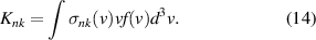
Standard image High-resolution imageThe acceleration specifically from electron impact ionization from the neutral ground state is given by , where the is the source frequency from the neutral ground state and Knk is the rate coefficient. The rate coefficient is given by the integral over velocity space, involving the cross-section of the process as a function of energy as in equation (14)

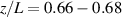
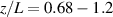
We can compare the deceleration due to just electron impact ionization and due to all populating processes. The far left plot in figure 10 shows the ratio of deceleration of the ion ground state to the deceleration of the ion metastable state due to all populating processes (blue) and just electron impact ionization (orange). The middle plot shows the ratio of the ion ground state density to the metastable state density, and the right plot shows the ratio of the rate coefficient of electron impact ionization from the neutral ground state to the ion ground state to the rate coefficient of that same process to the ion metastable state. Up until , the ratio of deceleration can be explained mostly by electron impact ionization. However, as the electron temperature decreases beyond , ionization directly to the metastable state becomes rare, as shown in figure 11. Meanwhile, spontaneous decays from higher states with lower velocities than the metastable state become the dominant cause of metastable deceleration (see figure 12). This contribution is sufficient to reduce the ratio of ground state to metastable state acceleration shown in figure 10(a).


Figure 10. Ratios of ground state ion to metastable state ion acceleration, population density, and rate coefficients from the neutral ground state along the HERMeS channel centerline.
![$5p^4(^3P_2)5d^2[4]_{7/2}$](https://content.cld.iop.org/journals/0963-0252/32/1/015009/revision2/psstacb00bieqn51.gif)
Download figure:
Standard image High-resolution image
Figure 11. Rate of metastable state ion creation by each process along the HERMeS channel centerline.
![$5p^4(^3P_2)5d^2[4]_{7/2}$](https://content.cld.iop.org/journals/0963-0252/32/1/015009/revision2/psstacb00bieqn52.gif)
Download figure:
Standard image High-resolution image
Figure 12. Acceleration of the metastable state from each populating process along the HERMeS channel centerline, downstream.
![$5p^4(^3P_2)5d^2[4]_{7/2}$](https://content.cld.iop.org/journals/0963-0252/32/1/015009/revision2/psstacb00bieqn53.gif)
Download figure:
Standard image High-resolution image3.2. SPT-100 channel centerline
The differences between the metastable and ground state ion velocities are less than 0.5 km s−1 for the HERMeS centerline test case, with smaller differences near the channel. However, it is important to consider additional test cases before generalizing from the HERMeS results. This section will investigate results using published simulation data of the SPT-100 thruster channel centerline (Test case 106 of the HYPICFLU hybrid model described in [18]). The discharge voltage and discharge current of the simulated test case are 300 V and 4.5 A, respectively. The SPT-100 was chosen because it has been studied extensively, and unlike HERMeS, it is not magnetically shielded, which leads to significant differences in the channel centerline profiles of plasma parameters. The thruster parameters of both the HERMeS channel centerline and the SPT-100 channel centerline are shown in figure 13, each normalized to their respective channel lengths for comparison. We acknowledge that there are some discrepancies between the SPT-100 simulation results used here and available experimental data [3], particularly the acceleration occurring fully within the channel of the thruster. However, the main goal is to demonstrate how the metastable-ground state velocity differential varies for different thruster test cases, and the SPT-100 simulations still serve as a useful test case even if the parameters do not accurately match the real thruster.

Figure 13. Thruster parameters along the channel centerline of the HERMeS and SPT-100 thrusters.
Download figure:
Standard image High-resolution imageThe resulting velocity and density profiles are shown in figure 14. Similar to the HERMeS channel centerline test case, the calculated non-metastable level velocity is close to the ground state ion velocity for the SPT-100 channel centerline. Also as before, the metastable state ions have slightly different velocities than the ground state ions primarily due to different rates at which the metastable ion state and ion ground state are populated by electron-impact transitions and CEX from the neutral ground state.
![$5p^4(^1D_2)5d^2[2]_{5/2}$](https://content.cld.iop.org/journals/0963-0252/32/1/015009/revision2/psstacb00bieqn58.gif)

Figure 14. Velocity (left) and density (right) profiles of each energy level along SPT-100 channel centerline.
Download figure:
Standard image High-resolution imageInvestigating these differences starting with non-metastable level , figure 15 shows that while there is a larger initial difference, the non-metastable state ion velocity moves back towards the ground state ion velocity. Again, electron excitation from the ground state is the dominant populating process.
![$5p^4(^1D_2)5d^2[2]_{5/2}$](https://content.cld.iop.org/journals/0963-0252/32/1/015009/revision2/psstacb00bieqn59.gif)

Figure 15. Left: difference between local axial velocity uz for non-metastable level ions, uzk , and ground state ions, , along the SPT-100 normalized channel axis compared to acceleration terms from the momentum equation. Right: axial populating rates for level ions.
![$5p^4(^1D_2)5d^2[2]_{5/2}$](https://content.cld.iop.org/journals/0963-0252/32/1/015009/revision2/psstacb00bieqn60.gif)

![$5p^4(^1D_2)5d^2[2]_{5/2}$](https://content.cld.iop.org/journals/0963-0252/32/1/015009/revision2/psstacb00bieqn62.gif)
Download figure:
Standard image High-resolution imageThe metastable ion velocities exceed the ground state ion velocity by up to 0.3 km s−1 for the state and up to 0.5 km s−1 for the state. For this case, the magnitude of deceleration of the metastable ion states is consistently lower than the magnitude of deceleration of the ion ground state, and thus the difference between the ground state and metastable ions becomes increasingly negative downstream, as shown in figure 16. Therefore, as with the HERMeS test case, the differences between the ground state ion velocity and the metastable ion velocities can be explained by the relative rates of deceleration which stem from population events from the slower neutral ground state.
![$5p^4(^3P_2)5d^2[4]_{7/2}$](https://content.cld.iop.org/journals/0963-0252/32/1/015009/revision2/psstacb00bieqn65.gif)
![$5p^4(^3P_2)5d^2[3]_{7/2}$](https://content.cld.iop.org/journals/0963-0252/32/1/015009/revision2/psstacb00bieqn66.gif)

Figure 16. Difference between metastable and ground state ion velocities (blue) versus source acceleration (black) for the state (left) and state (right) along the SPT-100 channel centerline.
![$5p^4(^3P_2)5d^2[4]_{7/2}$](https://content.cld.iop.org/journals/0963-0252/32/1/015009/revision2/psstacb00bieqn63.gif)
![$5p^4(^3P_2)5d^2[3]_{7/2}$](https://content.cld.iop.org/journals/0963-0252/32/1/015009/revision2/psstacb00bieqn64.gif)
Download figure:
Standard image High-resolution imageWe again focus on the metastable state . The deceleration from each populating process is shown in figure 17. Compared to the HERMeS test case in figure 9, electron impact ionization from the neutral ground state again is responsible for most of the deceleration, but the magnitude for the SPT-100 test case is about four times larger. The magnitude of deceleration is higher because the neutral density along the SPT-100 channel centerline is higher, and thus there are more populating events from the slower neutral ground state. The higher neutral density also leads to more deceleration of the ion ground state. Because the the deceleration of both the ground state and metastable state ions increase with higher neutral density, the difference between the magnitudes of deceleration will also increase with neutral density. This leads to a larger difference between the resulting ground state and metastable state ion velocities.
![$5p^4(^3P_2)5d^2[4]_{7/2}$](https://content.cld.iop.org/journals/0963-0252/32/1/015009/revision2/psstacb00bieqn69.gif)

Figure 17. Acceleration of the metastable state from each populating process along the SPT-100 channel centerline.
![$5p^4(^3P_2)5d^2[4]_{7/2}$](https://content.cld.iop.org/journals/0963-0252/32/1/015009/revision2/psstacb00bieqn67.gif)
Download figure:
Standard image High-resolution imageBy plotting the rate of metastable ion creation along the channel centerline from each populating process in figure 18, we see that the significance of metastable ion creation from the neutral ground state remains relatively constant compared to creation from other states inside the channel (up until ). After the channel exit, as the neutral population is depleted, the relative rate of metastable ion creation from the neutral ground state decreases. Again, although excitation from the ion ground state has the highest rate of metastable ion creation, the large differences between the metastable ion and neutral ground state velocity make electron impact ionization from the neutral ground state the most significant source of deceleration for the first portion of the channel centerline. As the rate of creation from the neutral ground state decreases, so does the magnitude of ion deceleration.


Figure 18. Rate of metastable state ion creation by each process along the SPT-100 channel centerline.
![$5p^4(^3P_2)5d^2[4]_{7/2}$](https://content.cld.iop.org/journals/0963-0252/32/1/015009/revision2/psstacb00bieqn68.gif)
Download figure:
Standard image High-resolution image3.3. HET-P70 thruster
So far, the differences between the metastable state ion velocities and the ground state ion velocity has been within 0.5 km s−1 for the HERMeS and SPT-100 thruster channel centerline, which indicates the metastable ion velocity can be used as a good approximation of the overall ion velocity. To explore the limits of this assumption, we look at a third test case of a HET-P70 lab thruster that may not be as optimized as either HERMeS or SPT-100. Some limited information on the plume of the HET-P70 thruster was tabulated by Zhu et al. The datapoints provided in the channel of the HET-P70 thruster for electron temperature, electron density, and neutral density were extrapolated to follow the general trends of the HERMeS thruster parameters. The potential, and resulting electric field were assumed to be the same magnitude for the HET-P70 as the HERMeS channel centerline. The ground state ion velocity was calculated following the method described in section 2.4. The generated set of input parameters for the HET-P70 channel centerline are shown in figure 19. The acceleration region is farther upstream in the HET-P70 thruster compared to HERMeS due to differences in magnetic field shape and lack of magnetic shielding.

Figure 19. Input parameters for the HET-P70 thruster channel centerline.
Download figure:
Standard image High-resolution imageThe resulting axial velocity and density profiles are shown in figure 20. As with the previous two test cases, the non-metastable state velocity is close to the ground state ion velocity. The metastable ion state velocities, however, are clearly further from the ion ground state velocity than the previous two test cases. Around , the ground state and non-metastable state velocities decrease, but the metastable ion velocities continue to rise, failing to capture this feature near the end of the acceleration zone.
![$5p^4(^1D_2)6d^2[2]_{5/2}$](https://content.cld.iop.org/journals/0963-0252/32/1/015009/revision2/psstacb00bieqn74.gif)


Figure 20. Velocity (left) and density (right) profiles of each energy level along the HET-P70 channel centerline.
Download figure:
Standard image High-resolution imageThe difference between the ground and metastable state ions along with the source acceleration along the channel centerline is shown in figure 21. For this HET-P70 case, since the neutral density is much higher, the magnitudes of deceleration experienced by each of the ground state and metastable state ions is greater than the previous two test cases. Because the difference between the deceleration of the ground state and metastable state ions also scales with neutral density, the difference between the velocity of each state is larger.

Figure 21. Difference between metastable and ground state ion velocities (blue) versus source acceleration (black) for the state (left) and state (right) along the HET-P70 channel centerline.
![$5p^4(^3P_2)5d^2[4]_{7/2}$](https://content.cld.iop.org/journals/0963-0252/32/1/015009/revision2/psstacb00bieqn71.gif)
![$5p^4(^3P_2)5d^2[3]_{7/2}$](https://content.cld.iop.org/journals/0963-0252/32/1/015009/revision2/psstacb00bieqn72.gif)
Download figure:
Standard image High-resolution imageTo further illustrate the increased significance of electron impact ionization from the neutral ground state for this third test case, the rate of metastable ion creation from each populating process in shown in figure 22. The relative rate of metastable ion creation from the neutral ground state is much higher than the previous two test cases, even exceeding the rate of creation from the ion ground state in the upstream part of the channel.

Figure 22. Rate of metastable state ion creation by each process along the HET-P70 channel centerline.
![$5p^4(^3P_2)5d^2[4]_{7/2}$](https://content.cld.iop.org/journals/0963-0252/32/1/015009/revision2/psstacb00bieqn73.gif)
Download figure:
Standard image High-resolution image4. Discussion
Relatively good agreement has been found between the ground state ion velocity and metastable ion velocities. Here, we discuss potential sources of error in both the CR model used and the overall approach to computing the metastable ion velocities. In the CR model, the electron energy distribution function is assumed to be Maxwellian. A departure from equilibrium would influence the collision rates. The CR model also assumes the plasma is optically thin. This may introduce some error, especially in the high-density regions. However, it has been shown that including photon absorption in the neutral xenon CR model led to a less than ten percent change in results for over the full range of Hall thruster-relevant parameters [14], and the impact for xenon ions is expected to be similar. We also acknowledge that there is some uncertainty in the cross sections. The CR model does not include CEX cross sections, and while we include ground state CEX in our 1D model calculation, we neglect metastable CEX for which we expect the effects to be small.
In the computational approach, a 1D fluid model is implemented. This does not account for beam divergence and for the gradient of the velocity radial component. The fluid model only accounts for the mean velocity, contrary to a kinetic model which would yield the full IVDF. Interpretation of the IVDFs measured by LIF is discussed in the following paragraph. The ion temperature is assumed to be zero so that we may neglect the ion pressure term in the momentum equation, which could lead to error in our mean velocity calculation. The atom velocity is assumed to be constant, and there may be other errors in the plasma parameters of each thruster used in the calculation. We have done a sensitivity study in which we increase or decrease electron density or electron temperature of the HERMeS thruster by 50 and have found that the difference between the metastable state and ground state ion velocities changes by at most 0.1 km s−1.

We have shown that transitions from the slower neutral ground state bring down the mean velocity of metastable ions and ground state ions compared to an ion that has been fully accelerated by the drop in electric potential. However, even a large discrepancy between the ground state and metastable ion mean velocity (as in section 3.3) will not necessarily cause a problem for the interpretation of LIF measurements because slow ions born from the neutral ground state often appear in LIF data as a low-velocity tail that is distinguishable from the main ion population. An example is shown in figure 23. The low-velocity tail affects the overall mean (first moment) of the IVDF but not the most probable velocity, so consideration of the most probable velocity (MPV), or calculation of the first moment over a limited range of ion velocities spanning the main IVDF peak only, allows for errors from ionization and CEX effects to be avoided. Considering the most probable velocity has been recommended in previous Hall thruster LIF studies [3, 27–29]. To quantify the impact of differences between metastable and ground state ion velocities on the overall shape of the measured IVDF, one would need to incorporate the CR model into a kinetic analysis.

Figure 23. IVDFs (Annotated) from Chaplin et al [30].
Download figure:
Standard image High-resolution image5. Conclusions and future work
In conclusion, we have quantitatively assessed the accuracy of using metastable xenon ion states for estimating ion velocities for a Hall thruster. Overall, our results show that the metastable state ion velocities along the channel centerline differ from the overall mean ion velocity by up to ∼0.5 km s−1 for two high efficiency thrusters with low neutral densities, but differ by as much as 1.7 km s−1 for a thruster with higher neutral density. This increased difference with increased neutral density is due to ionization of atoms in the slower neutral ground state consistently lowering the calculated mean velocity of the ground state and metastable state ions proportionally to the rate coefficient of the electron impact ionization to each state times the neutral ground state density, and also CEX lowering the mean velocity of the ion ground state. Therefore, the discrepancy between the ion ground state and metastable state velocities grows with neutral density.
These results were determined by modeling the velocity and density profiles of excited ion states using the Xe II CR model with a variety of thruster parameters as inputs. We see that for each thruster test case, the non-metastable state velocity matches the ground state ion velocity as expected, confirming that the computational approach is reasonable.
![$5p^4(^1D_2)5d^2[2]_{5/2}$](https://content.cld.iop.org/journals/0963-0252/32/1/015009/revision2/psstacb00bieqn77.gif)
The results show that for the HERMeS thruster channel centerline, the metastable ion state overestimates the ground state ion velocity by up to 0.05 km s−1 in the acceleration region, by as low as 0.02 km s−1 just downstream, and by up to 0.3 km s−1 further downstream. The other metastable ion state follows these same trends. At the start of the computational domain, this state underestimates the ground state ion velocity by about 0.015 km s−1, then overestimates it by up to 0.42 km s−1 just downstream of the acceleration region.
![$5p^4(^3P_2)5d^2[4]_{7/2}$](https://content.cld.iop.org/journals/0963-0252/32/1/015009/revision2/psstacb00bieqn78.gif)
![$5p^4(^3P_1)5d^2[3]_{7/2}$](https://content.cld.iop.org/journals/0963-0252/32/1/015009/revision2/psstacb00bieqn79.gif)
We observe similar trends with the SPT-100 thruster channel centerline. Here, the metastable ion state overestimates the ground state ion velocity by up to 0.22 km s−1 in the acceleration region, by as low as 0.2 km s−1 just downstream, and by up to 0.3 km s−1 further downstream. Again, the results for the other metastable ion state are similar, but the differences are shifted in the positive direction. These differences are slightly higher than observed for the HERMeS test case, but overall the first two test cases suggest that the metastable ion velocity can be a reliable estimate of the ground state ion velocity and can be used to identify important features such as location of the acceleration region.
![$5p^4(^3P_2)5d^2[4]_{7/2}$](https://content.cld.iop.org/journals/0963-0252/32/1/015009/revision2/psstacb00bieqn80.gif)
![$5p^4(^3P_1)5d^2[3]_{7/2}$](https://content.cld.iop.org/journals/0963-0252/32/1/015009/revision2/psstacb00bieqn81.gif)
However, in exploring the limits of this assumption, we do see a larger difference between the metastable and ground state ion velocity for the HET-P70 thruster channel centerline. Here, the metastable ion state velocities overestimate the ground state ion velocity by about 0.3 km s−1 for the state and 0.5 km s−1 for the state in the acceleration region, then underestimate the ground state ion velocity by up to 0.7 km s−1 for both metastable states. Further downstream, the metastable ion states overestimate the ground state ion velocity by about 1.2 km s−1 for the state and 1.7 km s−1 for the state. This test case has a much higher neutral density, and lower electron temperature and electron density. Therefore, one should be aware of the thruster plume parameters when analyzing LIF data.
![$5p^4(^3P_2)5d^2[4]_{7/2}$](https://content.cld.iop.org/journals/0963-0252/32/1/015009/revision2/psstacb00bieqn82.gif)
![$5p^4(^3P_1)5d^2[3]_{7/2}$](https://content.cld.iop.org/journals/0963-0252/32/1/015009/revision2/psstacb00bieqn83.gif)
![$5p^4(^3P_2)5d^2[4]_{7/2}$](https://content.cld.iop.org/journals/0963-0252/32/1/015009/revision2/psstacb00bieqn84.gif)
![$5p^4(^3P_1)5d^2[3]_{7/2}$](https://content.cld.iop.org/journals/0963-0252/32/1/015009/revision2/psstacb00bieqn85.gif)
The excitations from the slower neutral ground state consistently lower the calculated mean velocity of the metastable state ions, especially for thrusters with relatively high neutral densities in the plume. Potential future work would include taking a kinetic approach to calculate the full IVDF and thereby isolate the effects of ionization from the neutral ground state and CEX. Another path forward could be to explore other regions of the Hall thruster plume besides the channel centerline, such as the near-pole region. While the channel centerline was chosen for its relative simplicity, understanding the behavior of the metastable ions compared to the ground state ions in these other regions would also be of interest.
Acknowledgments
This research was carried out at University of California, Los Angeles (UCLA) in collaboration with employees of the Jet Propulsion Laboratory, California Institute of Technology (JPL). Part of this research was carried out at the Jet Propulsion Laboratory, California Institute of Technology, under a contract with the National Aeronautics and Space Administration (80NM0018D0004). We gratefully acknowledge the support from the NASA Space Technology Graduate Research Fellowship (Grant Number 80NSSC19K1177).
© 2022. California Institute of Technology. Government sponshorship acknowledged.
Data availability statement
The data that support the findings of this study are available upon reasonable request from the authors.