

Abstract
An extended reaction kinetics model (RKM) suitable for the analysis of weakly ionised, non-thermal argon plasmas with gas temperatures around 300 K at sub-atmospheric and atmospheric pressures is presented. It considers 23 different species including electrons as well as the ground state atom, an atomic and molecular ion, four excited molecular states, and 15 excited atomic states of argon, where all individual 1s and 2p states (in Paschen notation) are included as a separate species. This 23-species RKM involves 409 collision processes and radiative transitions and recent electron collision cross section data. It is evaluated by means of results of time- and space-dependent fluid modelling of argon discharges and their comparison with measured data for two different dielectric barrier discharge configurations as well as a micro-scaled atmospheric-pressure plasma jet setup. The results are also compared with those obtained by use of a previously established 15-species RKM involving only the two lumped 2p states 2p10...5 and  . It is found that the 23-species RKM shows generally better agreement with experimental data and provides more options for direct comparison with measurements than the frequently used 15-species RKM.
Export citation and abstract BibTeX RIS

Original content from this work may be used under the terms of the Creative Commons Attribution 4.0 licence. Any further distribution of this work must maintain attribution to the author(s) and the title of the work, journal citation and DOI.
1. Introduction
Different types of non-thermal argon plasmas have found widespread usage in various fields of plasma-related fundamental research as well as in applied plasma sciences, such as surface modification [1, 2], thin film deposition [3, 4], sterilisation [5, 6], food processing [7], biological and medical applications [8, 9]. The broad interdisciplinary interest in argon plasmas is one reason for the further development of reaction kinetics models (RKMs) for the theoretical description of the various processes in plasmas. RKMs enable a detailed analysis of the properties of electrons and the considered heavy particle species as well as the resulting plasma-initiated chemical processes.
The development of RKMs for the modelling of plasmas with different gas compositions requires the compilation of a list of species present in the plasma and the processes they take part in. At first glance, it may seem that it is sufficient to collect as many species and processes as possible to create an adequate model. However, one also has to take into account the sometimes limited knowledge of data on relevant collision processes and the number of spatial dimensions to be dealt with in the framework of the model description. Furthermore, a reasonable RKM considers only particles necessary for a certain study and avoids the accumulation of insignificant particles, which only increase the complexity of the model and computational requirements.
In many cases, a profound knowledge about the argon plasma behaviour under certain operating conditions can be of tremendous help and facilitates the selection of the appropriate RKM. For instance, it is known that the dominant ion in argon plasmas changes with the change of gas pressure due to the increasing relevance of charge transfer processes at higher pressures. The number density of the argon molecular ion  is small in comparison with the atomic ion Ar+ at lower pressure [10] and can be neglected in the reaction kinetics scheme like in [11–18]. At higher pressures, the
  ion plays an important role and needs to be included in the model. In addition to the pressure, the gas temperature should also be considered during the development of an RKM. Depending on the plasma type, it can range from a few tens of Kelvin [19] via room temperature [20] to a few thousand Kelvin [21]. Taking into account that rate coefficients depend on the gas temperature for a number of collision processes, e.g. for electron–ion recombination and charge-transfer processes [22, 23], it is very likely that the importance of these processes is not the same at different gas temperatures.
The adequate choice of a more simple or more complex RKM depends to a large extent on the type of specific research, its needs, and the availability of data on collision cross sections or rate coefficients. For example, a simple RKM considering only electron–neutral impact ionisation and electron–ion recombination has proven to be very effective in the study of pattern formation and dynamics of plasma filaments in a dielectric barrier discharge (DBD) [24, 25]. Furthermore, the same RKM has also found application in investigations of the temporal non-linear behaviour of atmospheric-pressure DBDs in argon, characterised by the appearance of period-doubling bifurcation, quasi-periodicity, or even chaos [26]. However, if the research aims to determine the number density of specific argon species, the RKM should include all relevant processes for the production and loss of these species. In such cases, the applied RKM can become more complicated with a large number of species and related processes.
The application of RKMs with a large number of species is often hardly feasible for spatial-temporal modelling due to the resulting extensive computing times. Therefore, combining multiple species into a lumped state is a common approach in complex RKMs. For example, the two metastable (m) states of argon, Ar[1s5] and Ar[1s3] (in Paschen notation), and the two resonant (r) states, Ar[1s4] and Ar[1s2], were combined into the effective species Arm and Arr, respectively, in [27]. The same procedure was applied in [28] for the development of a more complex RKM, in which argon atom levels higher than the 1s levels were also taken into account as one effective species Arp. An extensive collisional-radiative model consisting of the ground state, Ar[1p0], the four individual 1s states and 60 higher effective levels was developed by Bogaerts et al [29] for the analysis of an argon glow discharge.
As long as the spatial distributions of plasma properties are not in the focus of the study, zero-dimensional (global) models are commonly used for numerical modelling and analysis of the plasma. Given that the computational time for these models is comparatively short even for the most complex RKMs, the reaction kinetics scheme can contain as many processes as needed, provided that the corresponding data on rate coefficients are available. Some of the largest RKMs can be found in the zero-dimensional studies of argon plasmas with the admixture of different gases [30, 31].
Owing to the increasing development of spectroscopic instruments and techniques in recent years, highly resolved emission data have become readily available to laboratories worldwide. Particularly for argon plasmas, emission lines considering various transitions between the 1s and 2p levels obtained by high-resolution measurements have often been used for different analyses [32, 33]. Typically, the dominant emission of atmospheric-pressure argon discharges is given by radiative quenching of all ten 2p states resulting in line spectra approximately between 700 and 900 nm. In order to be able to understand the argon kinetics in atmospheric-pressure plasmas using a theoretical means in sufficient details and couple it with and validate it by experiments, a detailed description of the individual 2p level kinetics is certainly needed. This is especially the case, if the next step is to develop diagnostic methods for such plasmas using collision-radiative models. Nowadays, diagnostic methods based on the steady-state approximation are used dominantly [34]. Nevertheless, the highly transient character of atmospheric-pressure argon plasmas calls for RKMs, which can be used for the development of time-dependent (i.e. non-steady-state) collision-radiative models for advanced plasma diagnostics—in the far sub-nanosecond time scales for example, see [35, 36]. Therefore, the undoubted need for a model that can meet the above mentioned requirements was one of the main reasons for the development of a complex RKM, as it is proposed here.
The general intention of the manuscript is to present an RKM that can be applied for investigations of weakly ionised, non-thermal argon plasmas with gas temperatures around 300 K at sub-atmospheric and atmospheric pressures. This is the first and a crucial step to clarify the detailed kinetics for pure argon plasmas. It can further serve as a basis for the development of models applicable to different types of argon plasmas at various working conditions.
The proposed reaction kinetics scheme is based on that applied in [15] for analysing the influence of the kinetics of excited atoms on the characteristics of an inductively coupled low-pressure plasma in argon during the early afterglow as well as on the one introduced in [37] for the analysis of microdischarges in an asymmetric DBD in argon. The former distinguishes 16 states including the ground state, the 14 individual excited states Ar[1s5...2] and Ar[2p10...1] as well as the atomic ion of argon. The latter was also utilised in [38] for the analysis of a micro-scaled atmospheric-pressure plasma jet (μAPPJ). In [37], the four 1s5...2 excited states were included in the RKM as individual species, and the ten 2p10...1 levels were combined into the two lumped states Ar[2p] = Ar[2p10...5] and Ar[2p'] = Ar[2p4...1]. All higher atomic excited levels were lumped in one summed state Ar*[hl]. In addition to the atomic and the molecular ion, the four excited molecular argon states ![$\mathrm{A}{\mathrm{r}}_{\mathrm{2}}^{\ast }[{}^{\mathrm{3}}{\Sigma }_{\mathrm{u}}^{+},\mathrm{v}=\mathrm{0}]$](https://content.cld.iop.org/journals/0963-0252/31/12/125002/revision2/psstac9332ieqn4.gif) ,
, ![$\mathrm{A}{\mathrm{r}}_{\mathrm{2}}^{\ast }[{}^{\mathrm{1}}{\Sigma }_{\mathrm{u}}^{+},\mathrm{v}=\mathrm{0}]$](https://content.cld.iop.org/journals/0963-0252/31/12/125002/revision2/psstac9332ieqn5.gif) ,
, ![$\mathrm{A}{\mathrm{r}}_{\mathrm{2}}^{\ast }[{}^{\mathrm{3}}{\Sigma }_{\mathrm{u}}^{+},\mathrm{v}\gg \mathrm{0}]$](https://content.cld.iop.org/journals/0963-0252/31/12/125002/revision2/psstac9332ieqn6.gif) , and
, and ![$\mathrm{A}{\mathrm{r}}_{\mathrm{2}}^{\ast }[{}^{\mathrm{1}}{\Sigma }_{\mathrm{u}}^{+},\mathrm{v}\gg \mathrm{0}]$](https://content.cld.iop.org/journals/0963-0252/31/12/125002/revision2/psstac9332ieqn7.gif) , were also taken into account. It could be shown that this 15-species RKM involving 114 collisional and radiative processes is suitable for the modelling of different types of plasma under various conditions. However, comparison with experimental data did not always give satisfactory agreement, especially when the applied voltage is close to the breakdown voltage.
, were also taken into account. It could be shown that this 15-species RKM involving 114 collisional and radiative processes is suitable for the modelling of different types of plasma under various conditions. However, comparison with experimental data did not always give satisfactory agreement, especially when the applied voltage is close to the breakdown voltage.
The proposed extended RKM aims to overcome these issues. It takes into account 23 different species involved in 409 collisional and radiative processes. In addition to the increase of the number of species and reactions, it also uses more recent data, e.g. for the electron-impact collision cross sections when compared to the RKMs reported in [15, 37].
The applicability of this 23-species RKM is tested by comparing experimental data with results obtained by time-dependent, spatially one-dimensional fluid modelling of argon discharges under different conditions. For this purpose, the measured data of three different experimental setups are used. The first test case considers electrical measurements, measurements of the Ar[1s5] number density as well as phase-resolved optical emission spectroscopy (PROES) measurements performed on the Venturi-DBD system described in [39]. The second evaluation case is based on electrical measurements obtained for a DBD plasma source designed for the analysis of thin-film deposition using mixtures of argon and small amounts of hexamethyldisiloxane (HMDSO) or tetramethylsilane (TMS) as precursor [40–42]. As third test case, PROES measurements on the megahertz-driven μAPPJ studied in [38] are used for the comparison with modelling results. In addition, a direct comparison of results obtained by the proposed 23-species RKM with those obtained by using the previously established 15-species RKM [37] are presented and discussed.
The manuscript is organised as follows. A detailed description of the proposed 23-species RKM is given in section 2. The time- and space-dependent fluid-Poisson modelling approach used for testing the applicability of this RKM is described in section 3. Section 4 provides the comparison between modelling and experimental results. It also includes a discussion about differences between the results obtained by use of the proposed 23-species and the formerly established 15-species RKM. Conclusions are given in section 5.
2. Description of the RKM
In addition to electrons, the proposed RKM for argon takes into account the ground state of the atom, four individual 1s5...2 and ten 2p10...1 excited atomic states, four excited molecular states as well as the atomic and molecular ion. Furthermore, it considers energetically higher states than the 1s and 2p excited states as one lumped state Ar*[hl] with a statistical weight of 289. The statistical weight of the lumped state Ar*[hl] is determined taking into account all levels higher than the 2p levels for which electron-collision cross section data are available from the study of Zatsarinny et al [43, 44]. A complete list of argon species included in the 23-species RKM along with the corresponding energy levels is given in table 1. The included species participate in 409 processes presented in tables 2 and 3. The key difference in comparison to the above-mentioned 15-species RKM [37] is reflected in the treatment of the 2p excited states. In the 15-species RKM, 2p states from 2p10 to 2p5 and from 2p4 to 2p1 are grouped in the accumulated states Ar[2p] and Ar[2p'], respectively. In the proposed RKM, the ten 2p excited states are included as a separate species. The development of the 23-species RKM was supported by the publication of Zatsarinny et al [43], which contains extensive and more recent cross section data for electron-impact excitation processes that are used here for the determination of corresponding rate and transport coefficients of electrons.
Table 1. List of argon species considered in the model.
| Index | Species | Statistical weight | Energy level (eV) |
|---|---|---|---|
| 1 | Ar[1p0] | 1 | 0 |
| 2 | Ar[1s5] | 5 | 11.548 |
| 3 | Ar[1s4] | 3 | 11.624 |
| 4 | Ar[1s3] | 1 | 11.723 |
| 5 | Ar[1s2] | 3 | 11.828 |
| 6 | Ar[2p10] | 3 | 12.907 |
| 7 | Ar[2p9] | 7 | 13.076 |
| 8 | Ar[2p8] | 5 | 13.095 |
| 9 | Ar[2p7] | 3 | 13.153 |
| 10 | Ar[2p6] | 5 | 13.172 |
| 11 | Ar[2p5] | 1 | 13.273 |
| 12 | Ar[2p4] | 3 | 13.283 |
| 13 | Ar[2p3] | 5 | 13.302 |
| 14 | Ar[2p2] | 3 | 13.328 |
| 15 | Ar[2p1] | 1 | 13.480 |
| 16 | Ar*[hl] | 289 | 13.845 |
| 17 | Ar+ | 4 | 15.755 |
| 18 |
![$\mathrm{A}{\mathrm{r}}_{\mathrm{2}}^{\ast }[{}^{\mathrm{3}}{\Sigma }_{\mathrm{u}}^{+},\mathrm{v}=\mathrm{0}]$](https://content.cld.iop.org/journals/0963-0252/31/12/125002/revision2/psstac9332ieqn8.gif)
| 3 | 9.76 |
| 19 |
![$\mathrm{A}{\mathrm{r}}_{\mathrm{2}}^{\ast }[{}^{\mathrm{1}}{\Sigma }_{\mathrm{u}}^{+},\mathrm{v}=\mathrm{0}]$](https://content.cld.iop.org/journals/0963-0252/31/12/125002/revision2/psstac9332ieqn9.gif)
| 1 | 9.84 |
| 20 |
![$\mathrm{A}{\mathrm{r}}_{\mathrm{2}}^{\ast }[{}^{\mathrm{3}}{\Sigma }_{\mathrm{u}}^{+},\mathrm{v}\gg \mathrm{0}]$](https://content.cld.iop.org/journals/0963-0252/31/12/125002/revision2/psstac9332ieqn10.gif)
| 3 | 11.37 |
| 21 |
![$\mathrm{A}{\mathrm{r}}_{\mathrm{2}}^{\ast }[{}^{\mathrm{1}}{\Sigma }_{\mathrm{u}}^{+},\mathrm{v}\gg \mathrm{0}]$](https://content.cld.iop.org/journals/0963-0252/31/12/125002/revision2/psstac9332ieqn11.gif)
| 1 | 11.45 |
| 22 |

| 2 | 14.50 |
Table 2. Electron–neutral particle collision processes considered in the RKM. The kinetic energy range of the electron cross section data used is given in eV. Corresponding references are given in the fourth column.
| Index | Process | Energy range (eV) | References |
|---|---|---|---|
| Elastic electron collision | |||
| 1 | Ar[1p0] + e → Ar[1p0] + e | 0–200;  200 200 | [43]; [46] |
| Electron-impact excitation and de-excitation | |||
| 2, 3 | Ar[1p0] + e ↔ Ar[1s5] + e | 11.548–301 | [43] |
| 4, 5 | Ar[1p0] + e ↔ Ar[1s4] + e | 11.624–300;  300 300 | [43]; [46] |
| 6, 7 | Ar[1p0] + e ↔ Ar[1s3] + e | 11.723–301 | [43] |
| 8, 9 | Ar[1p0] + e ↔ Ar[1s2] + e | 11.828–300;  300 300 | [43]; [46] |
| 10, 11 | Ar[1p0] + e ↔ Ar[2p10] + e | 12.907–301 | [43] |
| 12, 13 | Ar[1p0] + e ↔ Ar[2p9] + e | 13.076–301 | [43] |
| 14, 15 | Ar[1p0] + e ↔ Ar[2p8] + e | 13.095–300;  300 300 | [43]; [46] |
| 16, 17 | Ar[1p0] + e ↔ Ar[2p7] + e | 13.153–301 | [43] |
| 18, 19 | Ar[1p0] + e ↔ Ar[2p6] + e | 13.172–300;  300 300 | [43]; [46] |
| 20, 21 | Ar[1p0] + e ↔ Ar[2p5] + e | 13.273–300;  300 300 | [43]; [46] |
| 22, 23 | Ar[1p0] + e ↔ Ar[2p4] + e | 13.283–301 | [43] |
| 24, 25 | Ar[1p0] + e ↔ Ar[2p3] + e | 13.302–300;  300 300 | [43]; [46] |
| 26, 27 | Ar[1p0] + e ↔ Ar[2p2] + e | 13.328–301 | [43] |
| 28, 29 | Ar[1p0] + e ↔ Ar[2p1] + e | 13.480–300;  300 300 | [43]; [46] |
| 30, 31 | Ar[1p0] + e ↔ Ar*[hl] + e | 13.845–300;  300 300 | [43]; [46] |
| 32, 33 | Ar[1s5] + e ↔ Ar[1s4] + e | 0.076–288;  288 288 | [43]; [47] |
| 34, 35 | Ar[1s5] + e ↔ Ar[1s3] + e | 0.175–288;  288 288 | [43]; [47] |
| 36, 37 | Ar[1s5] + e ↔ Ar[1s2] + e | 0.280–288;  288 288 | [43]; [47] |
| 38, 39 | Ar[1s5] + e ↔ Ar[2p10] + e | 1.359–288;  288 288 | [43]; [47] |
| 40, 41 | Ar[1s5] + e ↔ Ar[2p9] + e | 1.528–288;  288 288 | [43]; [47] |
| 42, 43 | Ar[1s5] + e ↔ Ar[2p8] + e | 1.547–288;  288 288 | [43]; [47] |
| 44, 45 | Ar[1s5] + e ↔ Ar[2p7] + e | 1.605–288;  288 288 | [43]; [47] |
| 46, 47 | Ar[1s5] + e ↔ Ar[2p6] + e | 1.624–288;  288 288 | [43]; [47] |
| 48, 49 | Ar[1s5] + e ↔ Ar[2p5] + e | 1.725–300 | [43] |
| 50, 51 | Ar[1s5] + e ↔ Ar[2p4] + e | 1.735–288;  288 288 | [43]; [47] |
| 52, 53 | Ar[1s5] + e ↔ Ar[2p3] + e | 1.754–288;  288 288 | [43]; [47] |
| 54, 55 | Ar[1s5] + e ↔ Ar[2p2] + e | 1.780–288;  288 288 | [43]; [47] |
| 56, 57 | Ar[1s5] + e ↔ Ar[2p1] + e | 1.932–300 | [43] |
| 58, 59 | Ar[1s5] + e ↔ Ar*[hl] + e | 2.297–288;  288 288 | [43, 44]; [47] |
| 60, 61 | Ar[1s4] + e ↔ Ar[1s3] + e | 0.099–288;  288 288 | [43]; [47] |
| 62, 63 | Ar[1s4] + e ↔ Ar[1s2] + e | 0.204–288;  288 288 | [43]; [47] |
| 64, 65 | Ar[1s4] + e ↔ Ar[2p10] + e | 1.283–288;  288 288 | [43]; [47] |
| 66, 67 | Ar[1s4] + e ↔ Ar[2p9] + e | 1.452–288;  288 288 | [43]; [47] |
| 68, 69 | Ar[1s4] + e ↔ Ar[2p8] + e | 1.471–288;  288 288 | [43]; [47] |
| 70, 71 | Ar[1s4] + e ↔ Ar[2p7] + e | 1.529–288;  288 288 | [43]; [47] |
| 72, 73 | Ar[1s4] + e ↔ Ar[2p6] + e | 1.548–288;  288 288 | [43]; [47] |
| 74, 75 | Ar[1s4] + e ↔ Ar[2p5] + e | 1.649–288;  288 288 | [43]; [47] |
| 76, 77 | Ar[1s4] + e ↔ Ar[2p4] + e | 1.659–288;  288 288 | [43]; [47] |
| 78, 79 | Ar[1s4] + e ↔ Ar[2p3] + e | 1.678–288;  288 288 | [43]; [47] |
| 80, 81 | Ar[1s4] + e ↔ Ar[2p2] + e | 1.704–288;  288 288 | [43]; [47] |
| 82, 83 | Ar[1s4] + e ↔ Ar[2p1] + e | 1.856–288;  288 288 | [43]; [47] |
| 84, 85 | Ar[1s4] + e ↔ Ar*[hl] + e | 2.221–288;  288 288 | [43, 44]; [47] |
| 86, 87 | Ar[1s3] + e ↔ Ar[1s2] + e | 0.105–288;  288 288 | [43]; [47] |
| 88, 89 | Ar[1s3] + e ↔ Ar[2p10] + e | 1.184–288;  288 288 | [43]; [47] |
| 90, 91 | Ar[1s3] + e ↔ Ar[2p9] + e | 1.353–288;  288 288 | [43]; [47] |
| 92, 93 | Ar[1s3] + e ↔ Ar[2p8] + e | 1.372–288;  288 288 | [43]; [47] |
| 94, 95 | Ar[1s3] + e ↔ Ar[2p7] + e | 1.430–288;  288 288 | [43]; [47] |
| 96, 97 | Ar[1s3] + e ↔ Ar[2p6] + e | 1.449–288;  288 288 | [43]; [47] |
| 98, 99 | Ar[1s3] + e ↔ Ar[2p5] + e | 1.550–288;  288 288 | [43]; [47] |
| 100, 101 | Ar[1s3] + e ↔ Ar[2p4] + e | 1.560–288;  288 288 | [43]; [47] |
| 102, 103 | Ar[1s3] + e ↔ Ar[2p3] + e | 1.579–288;  288 288 | [43]; [47] |
| 104, 105 | Ar[1s3] + e ↔ Ar[2p2] + e | 1.605–288;  288 288 | [43]; [47] |
| 106, 107 | Ar[1s3] + e ↔ Ar[2p1] + e | 1.757–288;  288 288 | [43]; [47] |
| 108, 109 | Ar[1s3] + e ↔ Ar*[hl] + e | 2.122–288;  288 288 | [43, 44]; [47] |
| 110, 111 | Ar[1s2] + e ↔ Ar[2p10] + e | 1.079–288;  288 288 | [43]; [47] |
| 112, 113 | Ar[1s2] + e ↔ Ar[2p9] + e | 1.248–288;  288 288 | [43]; [47] |
| 114, 115 | Ar[1s2] + e ↔ Ar[2p8] + e | 1.267–288;  288 288 | [43]; [47] |
| 116, 117 | Ar[1s2] + e ↔ Ar[2p7] + e | 1.325–288;  288 288 | [43]; [47] |
| 118, 119 | Ar[1s2] + e ↔ Ar[2p6] + e | 1.344–288;  288 288 | [43]; [47] |
| 120, 121 | Ar[1s2] + e ↔ Ar[2p5] + e | 1.445–288;  288 288 | [43]; [47] |
| 122, 123 | Ar[1s2] + e ↔ Ar[2p4] + e | 1.455–288;  288 288 | [43]; [47] |
| 124, 125 | Ar[1s2] + e ↔ Ar[2p3] + e | 1.474–288;  288 288 | [43]; [47] |
| 126, 127 | Ar[1s2] + e ↔ Ar[2p2] + e | 1.500–288;  288 288 | [43]; [47] |
| 128, 129 | Ar[1s2] + e ↔ Ar[2p1] + e | 1.652–288;  288 288 | [43]; [47] |
| 130, 131 | Ar[1s2] + e ↔ Ar*[hl] + e | 2.017–288;  288 288 | [43, 44]; [47] |
| 132, 133 | Ar[2p10] + e ↔ Ar[2p9] + e | 0.130–287;  287 287 | [43]; [47] |
| 134, 135 | Ar[2p10] + e ↔ Ar[2p8] + e | 0.153–287;  287 287 | [43]; [47] |
| 136, 137 | Ar[2p10] + e ↔ Ar[2p7] + e | 0.202–287;  287 287 | [43]; [47] |
| 138, 139 | Ar[2p10] + e ↔ Ar[2p6] + e | 0.225–287;  287 287 | [43]; [47] |
| 140, 141 | Ar[2p10] + e ↔ Ar[2p5] + e | 0.322–287;  287 287 | [43]; [47] |
| 142, 143 | Ar[2p10] + e ↔ Ar[2p4] + e | 0.323–287;  287 287 | [43]; [47] |
| 144, 145 | Ar[2p10] + e ↔ Ar[2p3] + e | 0.344–287;  287 287 | [43]; [47] |
| 146, 147 | Ar[2p10] + e ↔ Ar[2p2] + e | 0.368–287;  287 287 | [43]; [47] |
| 148, 149 | Ar[2p10] + e ↔ Ar[2p1] + e | 0.520–287;  287 287 | [43]; [47] |
| 150, 151 | Ar[2p10] + e ↔ Ar*[hl] + e | 0.938–287;  287 287 | [43]; [47] |
| 152, 153 | Ar[2p9] + e ↔ Ar[2p8] + e | 0.019–287;  287 287 | [43]; [47] |
| 154, 155 | Ar[2p9] + e ↔ Ar[2p7] + e | 0.072–287;  287 287 | [43]; [47] |
| 156, 157 | Ar[2p9] + e ↔ Ar[2p6] + e | 0.096–287;  287 287 | [43]; [47] |
| 158, 159 | Ar[2p9] + e ↔ Ar[2p5] + e | 0.192–287;  287 287 | [43]; [47] |
| 160, 161 | Ar[2p9] + e ↔ Ar[2p4] + e | 0.193–287;  287 287 | [43]; [47] |
| 162, 163 | Ar[2p9] + e ↔ Ar[2p3] + e | 0.214–287;  287 287 | [43]; [47] |
| 164, 165 | Ar[2p9] + e ↔ Ar[2p2] + e | 0.238–287;  287 287 | [43]; [47] |
| 166, 167 | Ar[2p9] + e ↔ Ar[2p1] + e | 0.390–287;  287 287 | [43]; [47] |
| 168, 169 | Ar[2p9] + e ↔ Ar*[hl] + e | 0.769–287;  287 287 | [43]; [47] |
| 170, 171 | Ar[2p8] + e ↔ Ar[2p7] + e | 0.049–287;  287 287 | [43]; [47] |
| 172, 173 | Ar[2p8] + e ↔ Ar[2p6] + e | 0.072–287;  287 287 | [43]; [47] |
| 174, 175 | Ar[2p8] + e ↔ Ar[2p5] + e | 0.169–287;  287 287 | [43]; [47] |
| 176, 177 | Ar[2p8] + e ↔ Ar[2p4] + e | 0.170–287;  287 287 | [43]; [47] |
| 178, 179 | Ar[2p8] + e ↔ Ar[2p3] + e | 0.191–287;  287 287 | [43]; [47] |
| 180, 181 | Ar[2p8] + e ↔ Ar[2p2] + e | 0.215–287;  287 287 | [43]; [47] |
| 182, 183 | Ar[2p8] + e ↔ Ar[2p1] + e | 0.367–287;  287 287 | [43]; [47] |
| 184, 185 | Ar[2p8] + e ↔ Ar*[hl] + e | 0.750–287;  287 287 | [43]; [47] |
| 186, 187 | Ar[2p7] + e ↔ Ar[2p6] + e | 0.023–287;  287 287 | [43]; [47] |
| 188, 189 | Ar[2p7] + e ↔ Ar[2p5] + e | 0.120–287;  287 287 | [43]; [47] |
| 190, 191 | Ar[2p7] + e ↔ Ar[2p4] + e | 0.121–287;  287 287 | [43]; [47] |
| 192, 193 | Ar[2p7] + e ↔ Ar[2p3] + e | 0.142–287;  287 287 | [43]; [47] |
| 194, 195 | Ar[2p7] + e ↔ Ar[2p2] + e | 0.166–287;  287 287 | [43]; [47] |
| 196, 197 | Ar[2p7] + e ↔ Ar[2p1] + e | 0.318–287;  287 287 | [43]; [47] |
| 198, 199 | Ar[2p7] + e ↔ Ar*[hl] + e | 0.692–287;  287 287 | [43]; [47] |
| 200, 201 | Ar[2p6] + e ↔ Ar[2p5] + e | 0.097–287;  287 287 | [43]; [47] |
| 202, 203 | Ar[2p6] + e ↔ Ar[2p4] + e | 0.098–287;  287 287 | [43]; [47] |
| 204, 205 | Ar[2p6] + e ↔ Ar[2p3] + e | 0.119–287;  287 287 | [43]; [47] |
| 206, 207 | Ar[2p6] + e ↔ Ar[2p2] + e | 0.143–287;  287 287 | [43]; [47] |
| 208, 209 | Ar[2p6] + e ↔ Ar[2p1] + e | 0.295–287;  287 287 | [43]; [47] |
| 210, 211 | Ar[2p6] + e ↔ Ar*[hl] + e | 0.673–287;  287 287 | [43]; [47] |
| 212, 213 | Ar[2p5] + e ↔ Ar[2p4] + e | 0.001–287;  287 287 | [43]; [47] |
| 214, 215 | Ar[2p5] + e ↔ Ar[2p3] + e | 0.022–287;  287 287 | [43]; [47] |
| 216, 217 | Ar[2p5] + e ↔ Ar[2p2] + e | 0.046–287;  287 287 | [43]; [47] |
| 218, 219 | Ar[2p5] + e ↔ Ar[2p1] + e | 0.198–287;  287 287 | [43]; [47] |
| 220, 221 | Ar[2p5] + e ↔ Ar*[hl] + e | 0.572–287;  287 287 | [43]; [47] |
| 222, 223 | Ar[2p4] + e ↔ Ar[2p3] + e | 0.019–287;  287 287 | [43]; [47] |
| 224, 225 | Ar[2p4] + e ↔ Ar[2p2] + e | 0.045–287;  287 287 | [43]; [47] |
| 226, 227 | Ar[2p4] + e ↔ Ar[2p1] + e | 0.197–287;  287 287 | [43]; [47] |
| 228, 229 | Ar[2p4] + e ↔ Ar*[hl] + e | 0.562–287;  287 287 | [43]; [47] |
| 230, 231 | Ar[2p3] + e ↔ Ar[2p2] + e | 0.024–287;  287 287 | [43]; [47] |
| 232, 233 | Ar[2p3] + e ↔ Ar[2p1] + e | 0.176–287;  287 287 | [43]; [47] |
| 234, 235 | Ar[2p3] + e ↔ Ar*[hl] + e | 0.543–287;  287 287 | [43]; [47] |
| 236, 237 | Ar[2p2] + e ↔ Ar[2p1] + e | 0.152–287;  287 287 | [43]; [47] |
| 238, 239 | Ar[2p2] + e ↔ Ar*[hl] + e | 0.517–287;  287 287 | [43]; [47] |
| 240, 241 | Ar[2p1] + e ↔ Ar*[hl] + e | 0.365–286;  286 286 | [43]; [47] |
| Electron-impact ionisation | |||
| 242 | Ar[1p0] + e → Ar+ + 2e | 15.755–10 000 | [48] |
| 243 | Ar[1s5] + e → Ar+ + 2e | ⩾4.207 | [47] |
| 244 | Ar[1s4] + e → Ar+ + 2e | ⩾4.131 | [47] |
| 245 | Ar[1s3] + e → Ar+ + 2e | ⩾4.032 | [47] |
| 246 | Ar[1s2] + e → Ar+ + 2e | ⩾3.927 | [47] |
| 247 | Ar[2p10] + e → Ar+ + 2e | ⩾2.848 | [47] |
| 248 | Ar[2p9] + e → Ar+ + 2e | ⩾2.679 | [47] |
| 249 | Ar[2p8] + e → Ar+ + 2e | ⩾2.660 | [47] |
| 250 | Ar[2p7] + e → Ar+ + 2e | ⩾2.602 | [47] |
| 251 | Ar[2p6] + e → Ar+ + 2e | ⩾2.583 | [47] |
| 252 | Ar[2p5] + e → Ar+ + 2e | ⩾2.482 | [47] |
| 253 | Ar[2p4] + e → Ar+ + 2e | ⩾2.472 | [47] |
| 254 | Ar[2p3] + e → Ar+ + 2e | ⩾2.453 | [47] |
| 255 | Ar[2p2] + e → Ar+ + 2e | ⩾2.427 | [47] |
| 256 | Ar[2p1] + e → Ar+ + 2e | ⩾2.275 | [47] |
| 257 | Ar*[hl] + e → Ar+ + 2e | ⩾1.910 | [47] |
| 258 |
![$\mathrm{A}{\mathrm{r}}_{\mathrm{2}}^{\ast }[{}^{\mathrm{3}}{\Sigma }_{\mathrm{u}}^{+},\mathit{v}\gg \mathrm{0}]+\mathrm{e}\to \mathrm{A}{\mathrm{r}}_{\mathrm{2}}^{+}+\mathrm{2}\mathrm{e}$](https://content.cld.iop.org/journals/0963-0252/31/12/125002/revision2/psstac9332ieqn125.gif)
| 3.230–50;  50 50 | [49]; [47] |
| 259 |
![$\mathrm{A}{\mathrm{r}}_{\mathrm{2}}^{\ast }[{}^{\mathrm{1}}{\Sigma }_{\mathrm{u}}^{+},\mathit{v}\gg \mathrm{0}]+\mathrm{e}\to \mathrm{A}{\mathrm{r}}_{\mathrm{2}}^{+}+\mathrm{2}\mathrm{e}$](https://content.cld.iop.org/journals/0963-0252/31/12/125002/revision2/psstac9332ieqn127.gif)
| 3.150–50;  50 50 | [49]; [47] |
| 260 |
![$\mathrm{A}{\mathrm{r}}_{\mathrm{2}}^{\ast }[{}^{\mathrm{3}}{\Sigma }_{\mathrm{u}}^{+},\mathit{v}=\mathrm{0}]+\mathrm{e}\to \mathrm{A}{\mathrm{r}}_{\mathrm{2}}^{+}+\mathrm{2}\mathrm{e}$](https://content.cld.iop.org/journals/0963-0252/31/12/125002/revision2/psstac9332ieqn129.gif)
| 4.740–50;  50 50 | [47] |
| 261 |
![$\mathrm{A}{\mathrm{r}}_{\mathrm{2}}^{\ast }[{}^{\mathrm{1}}{\Sigma }_{\mathrm{u}}^{+},\mathit{v}=\mathrm{0}]+\mathrm{e}\to \mathrm{A}{\mathrm{r}}_{\mathrm{2}}^{+}+\mathrm{2}\mathrm{e}$](https://content.cld.iop.org/journals/0963-0252/31/12/125002/revision2/psstac9332ieqn131.gif)
| 4.660–50;  50 50 | [47] |
Table 3. Recombination, heavy particle collisions and radiative processes included in the RKM. The rate coefficients of two-body, three-body and radiation processes are given in units of m3 s−1, m6 s−1 and s−1, respectively. The electron temperature Te = 2/(3kB ue) and gas temperature Tg are given in K, where kB and ue are the Boltzmann constant and mean electron energy, respectively. The unit for the gap width d is m.
| Index | Process | Rate coefficient | References |
|---|---|---|---|
| Electron–ion recombination | |||
| 262 |
![$\mathrm{A}{\mathrm{r}}_{\mathrm{2}}^{+}+\mathrm{e}\to \mathrm{A}\mathrm{r}[\mathrm{1}{\mathrm{s}}_{\mathrm{5}}]+\mathrm{A}\mathrm{r}[\mathrm{1}{\mathrm{p}}_{\mathrm{0}}]$](https://content.cld.iop.org/journals/0963-0252/31/12/125002/revision2/psstac9332ieqn133.gif)
|

| [22] × 0.8 [50] × 0.25 |
| 263 |
![$\mathrm{A}{\mathrm{r}}_{\mathrm{2}}^{+}+\mathrm{e}\to \mathrm{A}\mathrm{r}[\mathrm{1}{\mathrm{s}}_{\mathrm{4}}]+\mathrm{A}\mathrm{r}[\mathrm{1}{\mathrm{p}}_{\mathrm{0}}]$](https://content.cld.iop.org/journals/0963-0252/31/12/125002/revision2/psstac9332ieqn135.gif)
|

| [22] × 0.8 [50] × 0.25 |
| 264 |
![$\mathrm{A}{\mathrm{r}}_{\mathrm{2}}^{+}+\mathrm{e}\to \mathrm{A}\mathrm{r}[\mathrm{1}{\mathrm{s}}_{\mathrm{3}}]+\mathrm{A}\mathrm{r}[\mathrm{1}{\mathrm{p}}_{\mathrm{0}}]$](https://content.cld.iop.org/journals/0963-0252/31/12/125002/revision2/psstac9332ieqn137.gif)
|

| [22] × 0.8 [50] × 0.25 |
| 265 |
![$\mathrm{A}{\mathrm{r}}_{\mathrm{2}}^{+}+\mathrm{e}\to \mathrm{A}\mathrm{r}[\mathrm{1}{\mathrm{s}}_{\mathrm{2}}]+\mathrm{A}\mathrm{r}[\mathrm{1}{\mathrm{p}}_{\mathrm{0}}]$](https://content.cld.iop.org/journals/0963-0252/31/12/125002/revision2/psstac9332ieqn139.gif)
|

| [22] × 0.8 [50] × 0.25 |
| 266 |
![$\mathrm{A}{\mathrm{r}}_{\mathrm{2}}^{+}+\mathrm{e}\to \mathrm{A}\mathrm{r}[\mathrm{2}{\mathrm{p}}_{\mathrm{10}}]+\mathrm{A}\mathrm{r}[\mathrm{1}{\mathrm{p}}_{\mathrm{0}}]$](https://content.cld.iop.org/journals/0963-0252/31/12/125002/revision2/psstac9332ieqn141.gif)
|

| [22] × 0.2 [50] × 0.1 |
| 267 |
![$\mathrm{A}{\mathrm{r}}_{\mathrm{2}}^{+}+\mathrm{e}\to \mathrm{A}\mathrm{r}[\mathrm{2}{\mathrm{p}}_{\mathrm{9}}]+\mathrm{A}\mathrm{r}[\mathrm{1}{\mathrm{p}}_{\mathrm{0}}]$](https://content.cld.iop.org/journals/0963-0252/31/12/125002/revision2/psstac9332ieqn143.gif)
|

| [22] × 0.2 [50] × 0.1 |
| 268 |
![$\mathrm{A}{\mathrm{r}}_{\mathrm{2}}^{+}+\mathrm{e}\to \mathrm{A}\mathrm{r}[\mathrm{2}{\mathrm{p}}_{\mathrm{8}}]+\mathrm{A}\mathrm{r}[\mathrm{1}{\mathrm{p}}_{\mathrm{0}}]$](https://content.cld.iop.org/journals/0963-0252/31/12/125002/revision2/psstac9332ieqn145.gif)
|

| [22] × 0.2 [50] × 0.1 |
| 269 |
![$\mathrm{A}{\mathrm{r}}_{\mathrm{2}}^{+}+\mathrm{e}\to \mathrm{A}\mathrm{r}[\mathrm{2}{\mathrm{p}}_{\mathrm{7}}]+\mathrm{A}\mathrm{r}[\mathrm{1}{\mathrm{p}}_{\mathrm{0}}]$](https://content.cld.iop.org/journals/0963-0252/31/12/125002/revision2/psstac9332ieqn147.gif)
|

| [22] × 0.2 [50] × 0.1 |
| 270 |
![$\mathrm{A}{\mathrm{r}}_{\mathrm{2}}^{+}+\mathrm{e}\to \mathrm{A}\mathrm{r}[\mathrm{2}{\mathrm{p}}_{\mathrm{6}}]+\mathrm{A}\mathrm{r}[\mathrm{1}{\mathrm{p}}_{\mathrm{0}}]$](https://content.cld.iop.org/journals/0963-0252/31/12/125002/revision2/psstac9332ieqn149.gif)
|

| [22] × 0.2 [50] × 0.1 |
| 271 |
![$\mathrm{A}{\mathrm{r}}_{\mathrm{2}}^{+}+\mathrm{e}\to \mathrm{A}\mathrm{r}[\mathrm{2}{\mathrm{p}}_{\mathrm{5}}]+\mathrm{A}\mathrm{r}[\mathrm{1}{\mathrm{p}}_{\mathrm{0}}]$](https://content.cld.iop.org/journals/0963-0252/31/12/125002/revision2/psstac9332ieqn151.gif)
|

| [22] × 0.2 [50] × 0.1 |
| 272 |
![$\mathrm{A}{\mathrm{r}}_{\mathrm{2}}^{+}+\mathrm{e}\to \mathrm{A}\mathrm{r}[\mathrm{2}{\mathrm{p}}_{\mathrm{4}}]+\mathrm{A}\mathrm{r}[\mathrm{1}{\mathrm{p}}_{\mathrm{0}}]$](https://content.cld.iop.org/journals/0963-0252/31/12/125002/revision2/psstac9332ieqn153.gif)
|

| [22] × 0.2 [50] × 0.1 |
| 273 |
![$\mathrm{A}{\mathrm{r}}_{\mathrm{2}}^{+}+\mathrm{e}\to \mathrm{A}\mathrm{r}[\mathrm{2}{\mathrm{p}}_{\mathrm{3}}]+\mathrm{A}\mathrm{r}[\mathrm{1}{\mathrm{p}}_{\mathrm{0}}]$](https://content.cld.iop.org/journals/0963-0252/31/12/125002/revision2/psstac9332ieqn155.gif)
|

| [22] × 0.2 [50] × 0.1 |
| 274 |
![$\mathrm{A}{\mathrm{r}}_{\mathrm{2}}^{+}+\mathrm{e}\to \mathrm{A}\mathrm{r}[\mathrm{2}{\mathrm{p}}_{\mathrm{2}}]+\mathrm{A}\mathrm{r}[\mathrm{1}{\mathrm{p}}_{\mathrm{0}}]$](https://content.cld.iop.org/journals/0963-0252/31/12/125002/revision2/psstac9332ieqn157.gif)
|

| [22] × 0.2 [50] × 0.1 |
| 275 |
![$\mathrm{A}{\mathrm{r}}_{\mathrm{2}}^{+}+\mathrm{e}\to \mathrm{A}\mathrm{r}[\mathrm{2}{\mathrm{p}}_{\mathrm{1}}]+\mathrm{A}\mathrm{r}[\mathrm{1}{\mathrm{p}}_{\mathrm{0}}]$](https://content.cld.iop.org/journals/0963-0252/31/12/125002/revision2/psstac9332ieqn159.gif)
|

| [22] × 0.2 [50] × 0.1 |
| 276 | Ar+ + 2e → Ar*[hl] + e |

| [57] |
| 277 | Ar+ + e → Ar*[hl] + hν |
| [57] |
| Chemo-ionisation processes | |||
| 278 | Ar[1s5] + Ar[1s5] → Ar+ + e + Ar[1p0] | 1.20 × 10⁻¹⁵ | [54] |
| 279 | Ar[1s5] + Ar[1s4] → Ar+ + e + Ar[1p0] | 2.10 × 10⁻¹⁵ | [54] |
| 280 | Ar[1s5] + Ar[1s3] → Ar+ + e + Ar[1p0] | 4.20 × 10⁻¹⁵ | [54] |
| 281 | Ar[1s5] + Ar[1s2] → Ar+ + e + Ar[1p0] | 4.20 × 10⁻¹⁵ | [54] |
| 282 | Ar[1s4] + Ar[1s4] → Ar+ + e + Ar[1p0] | 2.10 × 10⁻¹⁵ | [54] |
| 283 | Ar[1s4] + Ar[1s3] → Ar+ + e + Ar[1p0] | 2.10 × 10⁻¹⁵ | [54] |
| 284 | Ar[1s4] + Ar[1s2] → Ar+ + e + Ar[1p0] | 2.10 × 10⁻¹⁵ | [54] |
| 285 | Ar[1s3] + Ar[1s3] → Ar+ + e + Ar[1p0] | 1.20 × 10⁻¹⁵ | [58] |
| 286 | Ar[1s3] + Ar[1s2] → Ar+ + e + Ar[1p0] | 2.10 × 10⁻¹⁵ | [54] |
| 287 | Ar[1s2] + Ar[1s2] → Ar+ + e + Ar[1p0] | 2.10 × 10⁻¹⁵ | [54] |
| Charge-transfer reaction | |||
| 288 |
![$\mathrm{A}{\mathrm{r}}^{+}+\mathrm{2}\mathrm{A}\mathrm{r}[\mathrm{1}{\mathrm{p}}_{\mathrm{0}}]\to \mathrm{A}{\mathrm{r}}_{\mathrm{2}}^{+}+\mathrm{A}\mathrm{r}[\mathrm{1}{\mathrm{p}}_{\mathrm{0}}]$](https://content.cld.iop.org/journals/0963-0252/31/12/125002/revision2/psstac9332ieqn163.gif)
|

| [23] |
| Quenching processes | |||
| 289 | Ar*[hl] + Ar[1p0] → Ar[2p1] + Ar[1p0] | 1.00 × 10⁻¹⁷ | Estimated |
| 290 | Ar[2p1] + Ar[1p0] → Ar[1s2] + Ar[1p0] | 4.00 × 10⁻¹⁸ | [59] × 0.25 |
| 291 | Ar[2p1] + Ar[1p0] → Ar[1s3] + Ar[1p0] | 4.00 × 10⁻¹⁸ | [59] ×0.25 |
| 292 | Ar[2p1] + Ar[1p0] → Ar[1s4] + Ar[1p0] | 4.00 × 10⁻¹⁸ | [59] ×0.25 |
| 293 | Ar[2p1] + Ar[1p0] → Ar[1s5] + Ar[1p0] | 4.00 × 10⁻¹⁸ | [59] ×0.25 |
| 294 | Ar[2p2] + Ar[1p0] → Ar[2p3] + Ar[1p0] | 5.00 × 10⁻¹⁹ | [60] |
| 295 | Ar[2p2] + Ar[1p0] → Ar[1s2] + Ar[1p0] | 1.32 × 10⁻¹⁷ | [61] ×0.25 |
| 296 | Ar[2p2] + Ar[1p0] → Ar[1s3] + Ar[1p0] | 1.32 × 10⁻¹⁷ | [61] ×0.25 |
| 297 | Ar[2p2] + Ar[1p0] → Ar[1s4] + Ar[1p0] | 1.32 × 10⁻¹⁷ | [61] ×0.25 |
| 298 | Ar[2p2] + Ar[1p0] → Ar[1s5] + Ar[1p0] | 1.32 × 10⁻¹⁷ | [61] ×0.25 |
| 299 | Ar[2p3] + Ar[1p0] → Ar[2p4] + Ar[1p0] | 2.75 × 10⁻¹⁷ | [60] |
| 300 | Ar[2p3] + Ar[1p0] → Ar[2p5] + Ar[1p0] | 3.00 × 10⁻¹⁹ | [60] |
| 301 | Ar[2p3] + Ar[1p0] → Ar[2p6] + Ar[1p0] | 4.40 × 10⁻¹⁷ | [60] |
| 302 | Ar[2p3] + Ar[1p0] → Ar[2p7] + Ar[1p0] | 1.40 × 10⁻¹⁸ | [60] |
| 303 | Ar[2p3] + Ar[1p0] → Ar[2p8] + Ar[1p0] | 1.90 × 10⁻¹⁸ | [60] |
| 304 | Ar[2p3] + Ar[1p0] → Ar[2p9] + Ar[1p0] | 8.00 × 10⁻¹⁹ | [60] |
| 305 | Ar[2p3] + Ar[1p0] → Ar[1s2] + Ar[1p0] | 8.52 × 10⁻¹⁸ | [60, 61] ×0.25 |
| 306 | Ar[2p3] + Ar[1p0] → Ar[1s3] + Ar[1p0] | 8.52 × 10⁻¹⁸ | [60, 61] ×0.25 |
| 307 | Ar[2p3] + Ar[1p0] → Ar[1s4] + Ar[1p0] | 8.52 × 10⁻¹⁸ | [60, 61] ×0.25 |
| 308 | Ar[2p3] + Ar[1p0] → Ar[1s5] + Ar[1p0] | 8.52 × 10⁻¹⁸ | [60, 61] ×0.25 |
| 309 | Ar[2p4] + Ar[1p0] → Ar[2p3] + Ar[1p0] | 2.30 × 10⁻¹⁷ | [60] |
| 310 | Ar[2p4] + Ar[1p0] → Ar[2p5] + Ar[1p0] | 7.00 × 10⁻¹⁹ | [60] |
| 311 | Ar[2p4] + Ar[1p0] → Ar[2p6] + Ar[1p0] | 4.80 × 10⁻¹⁸ | [60] |
| 312 | Ar[2p4] + Ar[1p0] → Ar[2p7] + Ar[1p0] | 3.20 × 10⁻¹⁸ | [60] |
| 313 | Ar[2p4] + Ar[1p0] → Ar[2p8] + Ar[1p0] | 1.40 × 10⁻¹⁸ | [60] |
| 314 | Ar[2p4] + Ar[1p0] → Ar[2p9] + Ar[1p0] | 3.30 × 10⁻¹⁸ | [60] |
| 315 | Ar[2p4] + Ar[1p0] → Ar[1s2] + Ar[1p0] | 4.90 × 10⁻¹⁸ | [60, 61] ×0.25 |
| 316 | Ar[2p4] + Ar[1p0] → Ar[1s3] + Ar[1p0] | 4.90 × 10⁻¹⁸ | [60, 61] ×0.25 |
| 317 | Ar[2p4] + Ar[1p0] → Ar[1s4] + Ar[1p0] | 4.90 × 10⁻¹⁸ | [60, 61] ×0.25 |
| 318 | Ar[2p4] + Ar[1p0] → Ar[1s5] + Ar[1p0] | 4.90 × 10⁻¹⁸ | [60, 61] ×0.25 |
| 319 | Ar[2p5] + Ar[1p0] → Ar[2p4] + Ar[1p0] | 1.70 × 10⁻¹⁸ | [60] |
| 320 | Ar[2p5] + Ar[1p0] → Ar[2p6] + Ar[1p0] | 1.13 × 10⁻¹⁷ | [60] |
| 321 | Ar[2p5] + Ar[1p0] → Ar[2p8] + Ar[1p0] | 9.50 × 10⁻¹⁸ | [60] |
| 322 | Ar[2p6] + Ar[1p0] → Ar[2p7] + Ar[1p0] | 4.10 × 10⁻¹⁸ | [60] |
| 323 | Ar[2p6] + Ar[1p0] → Ar[2p8] + Ar[1p0] | 6.00 × 10⁻¹⁸ | [60] |
| 324 | Ar[2p6] + Ar[1p0] → Ar[2p9] + Ar[1p0] | 1.00 × 10⁻¹⁸ | [60] |
| 325 | Ar[2p7] + Ar[1p0] → Ar[2p6] + Ar[1p0] | 2.50 × 10⁻¹⁸ | [60] |
| 326 | Ar[2p7] + Ar[1p0] → Ar[2p8] + Ar[1p0] | 1.43 × 10⁻¹⁷ | [60] |
| 327 | Ar[2p7] + Ar[1p0] → Ar[2p9] + Ar[1p0] | 2.33 × 10⁻¹⁷ | [60] |
| 328 | Ar[2p7] + Ar[1p0] → Ar[1s2] + Ar[1p0] | 9.22 × 10⁻¹⁸ | [60, 61] ×0.25 |
| 329 | Ar[2p7] + Ar[1p0] → Ar[1s3] + Ar[1p0] | 9.22 × 10⁻¹⁸ | [60, 61] ×0.25 |
| 330 | Ar[2p7] + Ar[1p0] → Ar[1s4] + Ar[1p0] | 9.22 × 10⁻¹⁸ | [60, 61] ×0.25 |
| 331 | Ar[2p7] + Ar[1p0] → Ar[1s5] + Ar[1p0] | 9.22 × 10⁻¹⁸ | [60, 61] ×0.25 |
| 332 | Ar[2p8] + Ar[1p0] → Ar[2p6] + Ar[1p0] | 3.00 × 10⁻¹⁹ | [60] |
| 333 | Ar[2p8] + Ar[1p0] → Ar[2p7] + Ar[1p0] | 8.00 × 10⁻¹⁹ | [60] |
| 334 | Ar[2p8] + Ar[1p0] → Ar[2p9] + Ar[1p0] | 1.82 × 10⁻¹⁷ | [60] |
| 335 | Ar[2p8] + Ar[1p0] → Ar[2p10] + Ar[1p0] | 1.00 × 10⁻¹⁸ | [60] |
| 336 | Ar[2p8] + Ar[1p0] → Ar[1s2] + Ar[1p0] | 6.68 × 10⁻¹⁸ | [60, 61] ×0.25 |
| 337 | Ar[2p8] + Ar[1p0] → Ar[1s3] + Ar[1p0] | 6.68 × 10⁻¹⁸ | [60, 61] ×0.25 |
| 338 | Ar[2p8] + Ar[1p0] → Ar[1s4] + Ar[1p0] | 6.68 × 10⁻¹⁸ | [60, 61] ×0.25 |
| 339 | Ar[2p8] + Ar[1p0] → Ar[1s5] + Ar[1p0] | 6.68 × 10⁻¹⁸ | [60, 61] ×0.25 |
| 340 | Ar[2p9] + Ar[1p0] → Ar[2p8] + Ar[1p0] | 6.80 × 10⁻¹⁸ | [60] |
| 341 | Ar[2p9] + Ar[1p0] → Ar[2p10] + Ar[1p0] | 5.10 × 10⁻¹⁸ | [60] |
| 342 | Ar[2p9] + Ar[1p0] → Ar[1s2] + Ar[1p0] | 1.18 × 10⁻¹⁷ | [60, 61] ×0.25 |
| 343 | Ar[2p9] + Ar[1p0] → Ar[1s3] + Ar[1p0] | 1.18 × 10⁻¹⁷ | [60, 61] ×0.25 |
| 344 | Ar[2p9] + Ar[1p0] → Ar[1s4] + Ar[1p0] | 1.18 × 10⁻¹⁷ | [60, 61] ×0.25 |
| 345 | Ar[2p9] + Ar[1p0] → Ar[1s5] + Ar[1p0] | 1.18 × 10⁻¹⁷ | [60, 61] ×0.25 |
| 346 | Ar[2p10] + Ar[1p0] → Ar[1s2] + Ar[1p0] | 5.00 × 10⁻¹⁸ | [61] ×0.25 |
| 347 | Ar[2p10] + Ar[1p0] → Ar[1s3] + Ar[1p0] | 5.00 × 10⁻¹⁸ | [61] ×0.25 |
| 348 | Ar[2p10] + Ar[1p0] → Ar[1s4] + Ar[1p0] | 5.00 × 10⁻¹⁸ | [61] ×0.25 |
| 349 | Ar[2p10] + Ar[1p0] → Ar[1s5] + Ar[1p0] | 5.00 × 10⁻¹⁸ | [61] ×0.25 |
| 350 | Ar[1s2] + Ar[1p0] → Ar[1s3] + Ar[1p0] | 4.76 × 10⁻²⁰ | [62] |
| 351 | Ar[1s3] + Ar[1p0] → Ar[1s4] + Ar[1p0] | 5.30 × 10⁻²¹ | [63] |
| 352 | Ar[1s4] + Ar[1p0] → Ar[1s5] + Ar[1p0] | 1.50 × 10⁻²⁰ | [64] |
| 353 | Ar[1s4] + 2Ar[1p0] ![$\to \mathrm{A}{\mathrm{r}}_{\mathrm{2}}^{\ast }[{}^{\mathrm{1}}{\Sigma }_{\mathrm{u}}^{+},\mathit{v}\gg \mathrm{0}]+\mathrm{A}\mathrm{r}[\mathrm{1}{\mathrm{p}}_{\mathrm{0}}]$](https://content.cld.iop.org/journals/0963-0252/31/12/125002/revision2/psstac9332ieqn165.gif)
| 1.50 × 10−45 | [64] |
| 354 | Ar[1s5] + Ar[1p0] → Ar[1s4] + Ar[1p0] | 2.50 × 10⁻²¹ | [64] |
| 355 | Ar[1s5] + Ar[1p0] → Ar[1p0] + Ar[1p0] | 1.50 × 10⁻²⁰ | [64] |
| 356 | Ar[1s5] + 2Ar[1p0]![$\to \mathrm{A}{\mathrm{r}}_{\mathrm{2}}^{\ast }[{}^{\mathrm{3}}\mathrm{S}_{\mathrm{u}}^{+},\mathit{v}\gg \mathrm{0}]+\mathrm{A}\mathrm{r}[\mathrm{1}{\mathrm{p}}_{\mathrm{0}}]$](https://content.cld.iop.org/journals/0963-0252/31/12/125002/revision2/psstac9332ieqn166.gif)
| 1.30 × 10−44 | [64] |
| 357 |
![$\mathrm{A}{\mathrm{r}}_{\mathrm{2}}^{\ast }[{}^{\mathrm{1}}{\Sigma }_{\mathrm{u}}^{+},\mathit{v}\gg \mathrm{0}]+\mathrm{A}\mathrm{r}[\mathrm{1}{\mathrm{p}}_{\mathrm{0}}]$](https://content.cld.iop.org/journals/0963-0252/31/12/125002/revision2/psstac9332ieqn167.gif)
![$\to \mathrm{A}{\mathrm{r}}_{\mathrm{2}}^{\ast }[{}^{\mathrm{1}}{\Sigma }_{\mathrm{u}}^{+},\mathit{v}=\mathrm{0}]+\mathrm{A}\mathrm{r}[\mathrm{1}{\mathrm{p}}_{\mathrm{0}}]$](https://content.cld.iop.org/journals/0963-0252/31/12/125002/revision2/psstac9332ieqn168.gif)
| 1.70 × 10⁻¹⁷ | [64] |
| 358 |
![$\mathrm{A}{\mathrm{r}}_{\mathrm{2}}^{\ast }[{}^{\mathrm{3}}{\Sigma }_{\mathrm{u}}^{+},\mathit{v}\gg \mathrm{0}]+\mathrm{A}\mathrm{r}[\mathrm{1}{\mathrm{p}}_{\mathrm{0}}]$](https://content.cld.iop.org/journals/0963-0252/31/12/125002/revision2/psstac9332ieqn169.gif)
![$\to \mathrm{A}{\mathrm{r}}_{\mathrm{2}}^{\ast }[{}^{\mathrm{3}}{\Sigma }_{\mathrm{u}}^{+},\mathit{v}=\mathrm{0}]+\mathrm{A}\mathrm{r}[\mathrm{1}{\mathrm{p}}_{\mathrm{0}}]$](https://content.cld.iop.org/journals/0963-0252/31/12/125002/revision2/psstac9332ieqn170.gif)
| 1.70 × 10⁻¹⁷ | [62, 64] |
| Radiative processes | |||
| 359 | Ar[1s4] → Ar[1p0] + hv |

| [56, 65, 66] |
| 360 | Ar[1s2] → Ar[1p0] + hv |

| [56, 65, 66] |
| 361 | Ar[2p10] → Ar[1s5] + hv | 1.89 × 10⁷ | [67] |
| 362 | Ar[2p10] → Ar[1s4] + hv | 5.43 × 10⁶ | [67] |
| 363 | Ar[2p10] → Ar[1s3] + hv | 9.80 × 10⁵ | [67] |
| 364 | Ar[2p10] → Ar[1s2] + hv | 1.90 × 10⁵ | [67] |
| 365 | Ar[2p9] → Ar[1s5] + hv | 3.31 × 10⁷ | [67] |
| 366 | Ar[2p8] → Ar[1s5] + hv | 9.28 × 10⁶ | [67] |
| 367 | Ar[2p8] → Ar[1s4] + hv | 2.15 × 10⁷ | [67] |
| 368 | Ar[2p8] → Ar[1s2] + hv | 1.47 × 10⁶ | [67] |
| 369 | Ar[2p7] → Ar[1s5] + hv | 5.18 × 10⁶ | [67] |
| 370 | Ar[2p7] → Ar[1s4] + hv | 2.50 × 10⁷ | [67] |
| 371 | Ar[2p7] → Ar[1s3] + hv | 2.43 × 10⁶ | [67] |
| 372 | Ar[2p7] → Ar[1s2] + hv | 1.06 × 10⁶ | [67] |
| 373 | Ar[2p6] → Ar[1s5] + hv | 2.45 × 10⁷ | [67] |
| 374 | Ar[2p6] → Ar[1s4] + hv | 4.90 × 10⁶ | [67] |
| 375 | Ar[2p6] → Ar[1s2] + hv | 5.03 × 10⁶ | [67] |
| 376 | Ar[2p5] → Ar[1s4] + hv | 4.02 × 10⁷ | [67] |
| 377 | Ar[2p5] → Ar[1s2] + hv | 1.00 × 10³ | [67] |
| 378 | Ar[2p4] → Ar[1s5] + hv | 6.25 × 10⁵ | [67] |
| 379 | Ar[2p4] → Ar[1s4] + hv | 2.20 × 10⁴ | [67] |
| 380 | Ar[2p4] → Ar[1s3] + hv | 1.86 × 10⁷ | [67] |
| 381 | Ar[2p4] → Ar[1s2] + hv | 1.39 × 10⁷ | [67] |
| 382 | Ar[2p3] → Ar[1s5] + hv | 3.80 × 10⁶ | [67] |
| 383 | Ar[2p3] → Ar[1s4] + hv | 8.47 × 10⁶ | [67] |
| 384 | Ar[2p3] → Ar[1s2] + hv | 2.23 × 10⁷ | [67] |
| 385 | Ar[2p2] → Ar[1s5] + hv | 6.39 × 10⁶ | [67] |
| 386 | Ar[2p2] → Ar[1s4] + hv | 1.83 × 10⁶ | [67] |
| 387 | Ar[2p2] → Ar[1s3] + hv | 1.17 × 10⁷ | [67] |
| 388 | Ar[2p2] → Ar[1s2] + hv | 1.53 × 10⁷ | [67] |
| 389 | Ar[2p1] → Ar[1s4] + hv | 2.36 × 10⁵ | [67] |
| 390 | Ar[2p1] → Ar[1s2] + hv | 4.45 × 10⁷ | [67] |
| 391 | Ar*[hl] → Ar[1p0] + hv |

| [56, 65, 66] |
| 392 | Ar*[hl] → Ar[1s5] + hv | 7.02 × 10⁴ | [66, 67] |
| 393 | Ar*[hl] → Ar[1s4] + hv | 4.21 × 10⁴ | [66, 67] |
| 394 | Ar*[hl] → Ar[1s3] + hv | 1.32 × 10⁴ | [66, 67] |
| 395 | Ar*[hl] → Ar[1s2] + hv | 4.11 × 10⁴ | [66, 67] |
| 396 | Ar*[hl] → Ar[2p10] + hv | 5.01 × 10⁵ | [66] |
| 397 | Ar*[hl] → Ar[2p9] + hv | 4.21 × 10⁵ | [66] |
| 398 | Ar*[hl] → Ar[2p8] + hv | 7.01 × 10⁵ | [66] |
| 399 | Ar*[hl] → Ar[2p7] + hv | 3.95 × 10⁵ | [66] |
| 400 | Ar*[hl] → Ar[2p6] + hv | 3.00 × 10⁵ | [66] |
| 401 | Ar*[hl] → Ar[2p5] + hv | 9.03 × 10⁴ | [66] |
| 402 | Ar*[hl] → Ar[2p4] + hv | 4.08 × 10⁵ | [66] |
| 403 | Ar*[hl] → Ar[2p3] + hv | 6.48 × 10⁵ | [66] |
| 404 | Ar*[hl] → Ar[2p2] + hv | 3.04 × 10⁵ | [66] |
| 405 | Ar*[hl] → Ar[2p1] + hv | 8.88 × 10⁴ | [66] |
| 406 |
![$\mathrm{A}{\mathrm{r}}_{\mathrm{2}}^{\ast }[{}^{\mathrm{1}}{\Sigma }_{\mathrm{u}}^{+},\mathit{v}\gg \mathrm{0}]\to \mathrm{2}\mathrm{A}\mathrm{r}[\mathrm{1}{\mathrm{p}}_{\mathrm{0}}]+\mathrm{h}\mathrm{v}$](https://content.cld.iop.org/journals/0963-0252/31/12/125002/revision2/psstac9332ieqn174.gif)
| 2.38 × 10⁸ | [62, 68] |
| 407 |
![$\mathrm{A}{\mathrm{r}}_{\mathrm{2}}^{\ast }[{}^{\mathrm{3}}{\Sigma }_{\mathrm{u}}^{+},\mathit{v}\gg \mathrm{0}]\to \mathrm{2}\mathrm{A}\mathrm{r}[\mathrm{1}{\mathrm{p}}_{\mathrm{0}}]+\mathrm{h}\mathrm{v}$](https://content.cld.iop.org/journals/0963-0252/31/12/125002/revision2/psstac9332ieqn175.gif)
| 2.00 × 10⁵ | [69] |
| 408 |
![$\mathrm{A}{\mathrm{r}}_{\mathrm{2}}^{\ast }[{}^{\mathrm{1}}{\Sigma }_{\mathrm{u}}^{+},\mathit{v}=\mathrm{0}]\to \mathrm{2}\mathrm{A}\mathrm{r}[\mathrm{1}{\mathrm{p}}_{\mathrm{0}}]+\mathrm{h}\mathrm{v}$](https://content.cld.iop.org/journals/0963-0252/31/12/125002/revision2/psstac9332ieqn176.gif)
| 2.38 × 10⁸ | [62, 68] |
| 409 |
![$\mathrm{A}{\mathrm{r}}_{\mathrm{2}}^{\ast }[{}^{\mathrm{3}}{\Sigma }_{\mathrm{u}}^{+},\mathit{v}=\mathrm{0}]\to \mathrm{2}\mathrm{A}\mathrm{r}[\mathrm{1}{\mathrm{p}}_{\mathrm{0}}]+\mathrm{h}\mathrm{v}$](https://content.cld.iop.org/journals/0963-0252/31/12/125002/revision2/psstac9332ieqn177.gif)
| 3.50 × 10⁵ | [64] |
The processes presented in table 2 include 261 electron collision processes with neutral argon species taking into account elastic collisions, excitation, de-excitation and ionisation. The rate coefficients for the processes in this table were determined by solving the steady-state electron Boltzmann equation in multi-term approximation using a generalised version of the method for weakly ionised plasmas presented in [45]. This method was adapted to include non-conservative electron collisions and the impact of the random motion of gas particles on elastic collision processes. The values for the reduced electric field (E/N ) and gas temperature (Tg) as well as the cross section data and further atomic data are used as input information. The calculated coefficients are placed in look-up tables and used in the RKM as a function of the mean electron energy.
To determine the rate coefficients for elastic electron collisions and electron-impact excitation processes up to around 200 eV and 300 eV of the kinetic electron energy Ukin, respectively, the collision cross sections reported in [43, 44] were utilised. For higher Ukin, the cross sections were mostly determined following Bethe approximation [47], except for elastic collisions and excitation processes of ground state argon atoms, where the data from [46] was considered. Cross section data for the electron-impact ionisation of argon in its ground state was taken from [48]. The analytic formula given by Vriens and Smeets [47] was applied for the determination of the electron-impact ionisation cross sections of excited argon atoms. The same analytic formula from [47] was utilised in the case of the ionisation of excited argon molecules, except that the cross section data for the high vibrational levels for Ukin ⩽ 50 eV was taken from [49]. The principle of detailed balance was applied for the determination of the cross sections of electron-impact de-excitation.
Furthermore, 16 electron–ion recombination processes, 81 heavy particle collision processes considering chemo-ionisation processes, charge-transfer reactions, and collisional quenching processes of excited argon species as well as 51 radiative processes are taken into consideration. They are listed in table 3. The rate coefficients for electron–ion dissociative recombination (DR) processes (index 262 to 275) depend on the electron and gas temperature according to [22]. The respective branching ratios are applied in accordance with the study of Royal and Orel [50]. In this work the authors state that the 1s atomic levels dominate the DR products, which is in agreement with the findings of Ramos et al [51]. It should be mentioned that an additional production channel of DR resulting in two argon ground state atoms is reported in [52, 53]. However, following the findings of Royal and Orel [50] that there is no evidence of these products, the mentioned production channel of DR is not included in the model. The further distribution of DR products considering the individual excited states is taken into account by assuming branching ratios of 0.25 and 0.1 for the four individual 1s5...2 and ten 2p10...1 states, respectively. Similar branching ratios were assumed in several collisional quenching processes of excited argon atoms. Concerning the chemo-ionisation processes, they involve only atomic excited states as described e.g. in [54]. Note that excimers can also take part in chemo-ionisation processes, which may become important at higher pressures [55]. However, excimer-induced chemo-ionisation is negligible for the conditions under consideration. Regarding the radiative processes, the resonance transitions from Ar[1s4], Ar[1s2] and Ar*[hl] levels to the ground state (i = 359, 360, 391) have high optical depth and the transition probabilities for these radiative processes are determined using the approximation of effective lifetime in agreement with [56]. This approach has already been successfully used in the studies of Becker et al [37] for the modelling of argon plasmas. Finally, it is important to say that the rate coefficients for all presented processes are suitable for the analysis of weakly ionised, non-thermal argon plasmas with gas temperatures around 300 K at sub-atmospheric and atmospheric pressures. For the investigations of much higher gas temperatures and pressures, the dependence of the rate coefficients on these parameters should be taken into account.
3. Fluid-Poisson model
Numerical studies of three different plasma sources were carried out to assess the applicability of the RKM presented in section 2. The first two cases consider different DBDs with plane-parallel configuration consisting of two electrodes, both covered by dielectric layers with a thickness Δ and a gas gap d, as illustrated in figure 1(a). The electrode on the left-hand side is powered by the sinusoidal voltage

with the amplitude U0 and frequency f, and the one on the right-hand side is grounded.

Figure 1. Schematic of the discharge geometries used in the modelling studies.
Download figure:
Standard image High-resolution imageIn the third test case, investigations were performed for the plasma of an atmospheric-pressure plasma jet with parallel electrodes separated by a gap d. A schematic representation of this setup is displayed in figure 1(b). In this case, the electrode on the right-hand side is powered by the sinusoidal voltage (1) and the one on the left-hand side is grounded.
3.1. Basic relations
The modelling studies were performed by means of a time-dependent, spatially one-dimensional fluid model based on a hydrodynamic description of the plasma, where the spatial variation takes place along the x-axis. The particle number densities of the species included in the RKM are obtained by solving their balance equation

Here, nj is the particle number density of the species j, Γj is the particle flux and Sj denotes the source term, which describes the gain and loss of particles in the plasma due to collisional and radiative processes. The spatiotemporal evolution of the mean electron energy ue is described by the energy balance equation

where we = ne ue and Qe denote the energy density and energy flux of electrons, respectively. The first term on the right-hand side of equation (3) represents the power input from the electric field and the second term describes the gain and loss of electron energy due to the different particle collision processes listed in tables 2 and 3.
In addition, the applied fluid model takes into account Poisson's equation

for the determination of the electric potential, Φ(x, t), and electric field, E(x, t) = −∂Φ(x, t)/∂x. Here, ɛr and ɛ0 are the relative and vacuum permittivity and qj is the particle charge.
For the determination of the fluxes of heavy particles, the common drift–diffusion approximation

is applied. Here, bj and Dj represent the mobility and diffusion coefficient of species j, respectively, and the function sgn(qj ) determines the sign of qj . The electron particle and energy flux are expressed by the relations


These relations were obtained by an expansion of the electron velocity distribution function (EVDF) in Legendre polynomials and the derivation of the first four moment equations from the Boltzmann equation of the electrons [70, 71]. The dissipation frequencies of the momentum (νe) and energy  flux as well as the transport coefficients ξ0, ξ2,
  , and
, and  are given as integrals of the isotropic part f0 and the first two contributions f1 and f2 to the anisotropy of the EVDF over the kinetic energy of the electrons as detailed in [72].
The transport coefficients for electrons were determined in the same way as the rate coefficients by solving their steady-state Boltzmann equation in multi-term approximation. The values of rate and transport coefficients of the electrons were used in the fluid-Poisson model as a function of the mean electron energy [73] (local-mean-energy approximation).
Notice that the present modelling approach does not include the impact of superelastic collisions of electrons on the EVDF. The influence of these processes can be taken into account similar to e.g. [74]. Furthermore, it should be mentioned that the present model does not couple self-consistently the time-dependent, spatially one-dimensional fluid-Poisson equations with the solution of the time- and space-dependent electron Boltzmann equation because of the large complexity of that approach and the expected enormous computational expenditure. Corresponding self-consistent approaches were reported e.g. in [75–79].
The mobilities of atomic and molecular argon ions were applied as functions of the reduced electric field E/N considering the data of [80, 81] and their diffusion coefficients were obtained using Einstein's relation [57]. The diffusion coefficients for the metastable argon atoms, Ar[1s5] and Ar[1s3], were determined according to NDm = 1.7 × 1018 cm−1 s−1 [80], where N is the background gas density.
3.2. Boundary conditions
In order to solve the set of equations (2)–(7), appropriate conditions were applied at the plasma-facing surfaces. Flux boundary conditions for electrons, heavy particles and the electron energy density as well as the emission of secondary electrons caused by ions impinging onto the walls were considered in accordance with [37, 82, 83]. Furthermore, surface charge accumulation at the dielectric surfaces was considered for the calculation of the electric field and potential in the test cases 1 and 2 dealing with DBDs (cf figure 1(a)).
4. Results and discussion
The modelling studies of three specific experimental setups with different characteristics and operating conditions were performed to evaluate the 23-species RKM presented in section 2. In the first test case, the analysed plasma source is part of the Venturi-DBD system used in [39, 84, 85]. The investigations are conducted for the gas pressure of 300 mbar and applied sinusoidal voltage with an amplitude of 1.5 kV and a frequency of 24 kHz corresponding to a period T = 41.7 μs. In the second test case, the study is carried out for an atmospheric-pressure DBD used to analyse the formation of thin polymer films in mixtures of argon with small amounts of HMDSO or TMS [40–42]. The analysed DBD in pure argon is driven by a sinusoidal voltage with an amplitude of 4 kV and a frequency of 86.2 kHz (T = 11.6 μs). The third evaluation case deals with a μAPPJ setup operated at the applied powers of 0.6 W and 1.3 W and the frequency f = 27.12 MHz (T = 36.9 ns). The discharge parameters used for the model calculations of the three setups are given in table 4.
Table 4. Discharge parameters for test case 1 (section 4.1), 2 (section 4.2), and 3 (section 4.3).
| Discharge parameter | Test case 1 | Test case 2 | Test case 3 |
|---|---|---|---|
| Gap d | 3 mm | 1 mm | 1.3 mm |
| Electrode area A | 7.62 cm2 | 8 cm2 | 0.2 cm2 |
| Dielectrics | Quartz | Borofloat glass | — |
| ɛr = 3.75 | ɛr = 4.6 | — | |
| Thickness of dielectric plate Δ | 1 mm | 2 mm | — |
| Applied voltage amplitude U0 | 1.5 kV | 4 kV | — |
| Applied power P | — | — | 0.6 and 1.3 W |
| Frequency f | 24 kHz | 86.2 kHz | 27.12 MHz |
| Pressure p | 300 mbar | 1 atm | 1 atm |
| Gas temperature Tg | 300 K | 300 K | 350 K |
| Gas purity | 99.999% | 99.9999% | 99.999% |
4.1. Test case 1
The considered DBD cell consists of two copper electrodes, both covered by 1 mm thick quartz dielectrics. The distance between the dielectric surfaces is d = 3 mm. The electrodes have rectangular shape with a length of 6.6 cm and width of 1.1 cm and provide the discharge area A = 7.62 cm2. The DBD is enclosed by a frame made of poly(methyl methacrylate) with quartz side panels, which make the discharge accessible for optical measurements. At the inlet of the plasma source, argon gas with a purity of 99.999% (Ar 5.0) [86] enters through a variable throttle valve (SS-1RS6MM, Swagelok, USA). The gas flow is driven through the system by a Venturi pump (VP00-060H, Vaccon Company Inc., USA) placed at the outlet of the plasma source. The measurements of the applied voltage and electrical current were performed by means of a 75 MHZ high-voltage probe (P6015A, Tektronix Inc., USA) and a current probe (TCP0030, Tektronix Inc., USA), respectively. The measured voltage signals at the powered electrode during the discharge were used as input for the modelling studies.
The modelling of this DBD was performed with the help of COMSOL Multiphysics® software [87] using the time-dependent solver. The system of partial differential equations (2)–(7) was solved by the finite element method using linear and quadratic Lagrange elements for the fluid equations (2) and (3) and Poisson's equation (4), respectively. The computational domain consists of a plasma region and two dielectric parts (cf figure 1(a)). In the plasma region, a non-uniform mesh with 1500 elements was employed, whose size decreases from the middle of the domain towards the dielectric walls. In both dielectric regions, a uniform mesh with 50 elements was used in accordance with [88]. For all calculations, the time step was adaptively determined considering the maximum relative error tolerance of 10−4. The model calculations were performed until a stable periodic state of the discharge was reached. The initial number density of electrons was 2 × 10¹² m−3 and the number densities of atomic and molecular ions were 1 × 10¹² m−3, assuring quasi-neutrality at the beginning of the calculations. An initial mean electron energy of 3 eV and zero potential in the gap were assumed.
The calculated spatiotemporal evolution of the electron number density and the temporal course of the discharge current

in the first seven voltage periods obtained by use of the 23-species RKM is shown in figure 2. It can be seen that the electron density exhibits a symmetric behaviour with respect to both half-periods of the applied voltage after few periods. Approximately equal intensities of positive and negative current peaks indicate that the calculated discharge current follows the same behaviour.
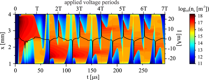
Figure 2. Spatiotemporal variation of the electron number density and temporal evolution of the discharge current obtained by use of the 23-species RKM in the first seven voltage periods at p = 300 mbar, U0 = 1.5 kV and f = 24 kHz (T = 41.7 μs).
Download figure:
Standard image High-resolution imageThe corresponding comparison of the measured and calculated current in the stable periodic state of the discharge represented in figure 3 shows that the measured results are very well described by the model calculation using the 23-species RKM. In addition to the good prediction of the time of the breakdown occurrence, the symmetry of the calculated current is also confirmed by the experimental results. It is important to note that the 15-species RKM could not be applied under the given conditions to analyse the discharge behaviour because the applied voltage was too low to ignite the discharge.
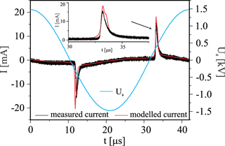
Figure 3. Periodic behaviour of the measured and calculated discharge current at the conditions in figure 2. Zero value of the time axis corresponds to t = 0.3 ms (7.25T ).
Download figure:
Standard image High-resolution imageIn order to reveal the reasons for different results obtained by means of the 15-species and 23-species RKM, their temporal evolutions of the spatially averaged mean electron energy  and electron number density
  during the first voltage period are displayed in figure 4. Here and in the following, the spatially averaged value
  of a property g(x, t) is determined according to

Figure 4(a) shows that the mean electron energy predicted by both RKMs increases synchronously with increasing energy input during the first 0.7 μs. Afterwards,  obtained by use of the 23-species RKM shows a faster increase with increasing time. A quite similar behaviour is noticed from the comparison of
  in figure 4(b), except for that the number densities obtained by both RKMs begin to differ after t = 1.4 μs. This means that at t = 1.4 μs the electron number densities are still approximately equal, while the mean electron energies are already different. In the further temporal course, larger differences between the results of the 15-species and 23-species RKM are found for
  and
and  . In particular, the results obtained by the 15-species RKM make clear that the electron number density remains too low to lead to ignition of the DBD.

Figure 4. Temporal evolution of the spatially averaged mean electron energy  (a) and electron number density
  (b) obtained by use of the 15-species and 23-species RKM during the first voltage period at p = 300 mbar, U0 = 1.5 kV and f = 24 kHz.
Download figure:
Standard image High-resolution imageFigure 5 shows the corresponding spatial variation of the number density and mean energy of the electrons in the gap at the time t = 1.4 μs. The electron number densities determined by both models are almost equal. They exhibit a maximum close to the momentary anode at x = 1.0 mm followed by a continuous decrease towards the momentary cathode at x = 4.0 mm. The mean electron energy is almost constant along the gap. The one obtained by the 23-species RKM is larger by about 0.2 eV than that obtained by the 15-species RKM. Electron-impact excitation processes of ground state argon atoms were found to be responsible for different electron energy losses at the present conditions resulting in different values of the mean electron energy.
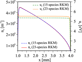
Figure 5. Spatial distributions of the electron number density and mean electron energy in the gap at the time t = 1.4 μs obtained by the 15-species and 23-species RKM at the conditions in figure 4.
Download figure:
Standard image High-resolution imageIn order to analyse the electron energy loss due to electron-impact excitation of Ar[1p0] in more detail, the corresponding frequencies of electron energy loss ![${\tilde{\nu }}_{\mathrm{e},i}^{\mathrm{L}}={\varepsilon }_{i}{k}_{i}{n}_{\text{Ar}[1\text{p}0]}$](https://content.cld.iop.org/journals/0963-0252/31/12/125002/revision2/psstac9332ieqn190.gif) are displayed as a function of the mean electron energy ue in figure 6(a). Here, i denotes the index of the process in table 2 and ɛi
and ki
are the electron energy loss and the rate coefficient of the process i, respectively. For a better presentation and to allow a direct comparison between the data of the 15-species and 23-species RKM, the frequencies of specific processes are summed according to the formula ∑i
ɛi
ki
nAr[1p0]. In particular, the electron energy loss frequencies due to electron-impact excitation processes of Ar[1p0] to the 1s levels (i = 2, 4, 6, 8), the 2p levels from 2p10 to 2p5 (i = 10, 12, 14, 16, 18, 20) and the 2p' levels from 2p4 to 2p1 (i = 22, 24, 26, 28) are shown and denoted by
are displayed as a function of the mean electron energy ue in figure 6(a). Here, i denotes the index of the process in table 2 and ɛi
and ki
are the electron energy loss and the rate coefficient of the process i, respectively. For a better presentation and to allow a direct comparison between the data of the 15-species and 23-species RKM, the frequencies of specific processes are summed according to the formula ∑i
ɛi
ki
nAr[1p0]. In particular, the electron energy loss frequencies due to electron-impact excitation processes of Ar[1p0] to the 1s levels (i = 2, 4, 6, 8), the 2p levels from 2p10 to 2p5 (i = 10, 12, 14, 16, 18, 20) and the 2p' levels from 2p4 to 2p1 (i = 22, 24, 26, 28) are shown and denoted by  ,
,  and
and  , respectively. It can be noticed that all frequencies used in the 23-species RKM are smaller than those of the 15-species RKM above ue = 5 eV. This implies that the 23-species RKM predicts less electron energy loss due to excitation processes with Ar[1p0] atoms. It is also a direct consequence of the use of more recent data on electron-impact collision cross sections in the 23-species RKM when compared to the 15-species RKM [37].

Figure 6. Frequencies of electron energy loss (a) ( —red lines,
  —blue lines,
  —green lines) and electron gain
  (b) as function of the mean electron energy at p = 300 mbar.
Download figure:
Standard image High-resolution imageAlthough the difference between the mean electron energies presented in figure 5 is only around 0.2 eV in main parts of the discharge region, the change of the electron particle gain frequency due to ionisation of ground state argon atoms, ![${\nu }_{\mathrm{e},\mathrm{1}{\mathrm{p}}_{\mathrm{0}}}^{\mathrm{G}}={k}_{242}{n}_{\text{Ar}[1\text{p}0]}$](https://content.cld.iop.org/journals/0963-0252/31/12/125002/revision2/psstac9332ieqn198.gif) , can become quite large. Figure 6(b) shows the corresponding frequencies of the 15-species and 23-species RKM as function of ue in the range from 5 eV to 6 eV. Generally, the presented frequencies show a similar monotonously increasing behaviour with increasing ue. In particular, the rapid increase of the mean electron energy between 5.3 and 5.5 eV by only 0.1 eV is accompanied by an increase of
, can become quite large. Figure 6(b) shows the corresponding frequencies of the 15-species and 23-species RKM as function of ue in the range from 5 eV to 6 eV. Generally, the presented frequencies show a similar monotonously increasing behaviour with increasing ue. In particular, the rapid increase of the mean electron energy between 5.3 and 5.5 eV by only 0.1 eV is accompanied by an increase of  by one order of magnitude. Therefore, the production of electrons in the case of the 23-species RKM is higher, taking into account that the generation of electrons is largely controlled by the aforementioned process.
Furthermore, a comparison between the calculated and measured number densities of the metastable Ar[1s5] atom is performed. For that purpose, a laser atom absorption spectroscopy (LAAS) system (EasyLAAS, neoplas control GmbH, Germany) with a 200 MHz photodetector (HCA-S, Femto, Germany) was used for the time-dependent absorption measurements at the wavelength of 811.53 nm, which corresponds to the  –
– transition. Details regarding the experimental setup are given in [89]. The measurements were performed in the middle of the gap, i.e. at x = 2.5 mm. Figure 7 shows the results of the Ar[1s5] number densities, corresponding calculated rates of main gain and loss processes of Ar[1s5] as well as the mean electron energy ue(x = 2.5 mm, t) during one period of the applied voltage Ua(t) in the periodic state of the discharge.

Figure 7. Periodic behaviour of the measured and calculated Ar[1s5] number density (a), calculated rates of main gain processes of Ar[1s5] and the mean electron energy ue (b) as well as rates of main loss processes of Ar[1s5] (c); i is the index of the processes in the tables 2 and 3. The results are obtained in the middle of the gap (x = 2.5 mm) at the conditions in figure 3.
Download figure:
Standard image High-resolution imageFigure 7(a) demonstrates clearly that the measured temporal evolution of the Ar[1s5] number density is very well described by the fluid-Poisson model using the 23-species RKM. The good agreement confirms an adequate choice of the processes defining the gain and loss of Ar[1s5] atoms as well as appropriate values of their rate coefficients in the modelling approach.
As it can be seen from figure 7(b), the mean electron energy reaches its largest values shortly before breakdown. Here, the direct electron-impact excitation process Ar[1p0] + e → Ar[1s5] + e (i = 2) is mostly responsible for the production of Ar[1s5] during the ignition phase. With breakdown, the mean electron energy decreases rapidly leading to a much smaller production of Ar[1s5] atoms. Note that there is a continuous contribution to the production of Ar[1s5] atoms due to the quenching (i = 293 and 352) and de-excitation (i = 33) of higher levels. This is compensated by the loss in two- and three-body quenching processes (i = 354–356).
Data of PROES measurements for the setup under consideration provide the possibility for an additional validation of the proposed 23-species RKM. The PROES setup used in the experimental studies includes a CCD camera (PicoStar HR12, LaVision GmbH, Germany) with a resolution of 520 × 520 pixels connected to an imaging spectrograph (Shamrock 750, Andor, United Kingdom) with a width of the entrance slit of 200 μm and a grating constant of 600 mm−1. Further details of the PROES measurements can be found in [89].
The measurements reveal the spatiotemporal dynamics of Ar[2p1] atoms in the gap based on the emission at the wavelength of 750.39 nm, which corresponds to the transition from Ar[2p1] to Ar[1s2]. The experimental results are presented in figures 8(a) and (b). They correspond to the emission during the breakdown events in the first and second half of the applied voltage period in the stable state of the discharge, respectively. Zero values of the time axis represent the moment when the magnitude of the discharge current reaches its maximum value. Since the regions with the highest intensity of light emission correspond to the largest production of Ar[2p1] atoms, the rate of production of Ar[2p1] due to all electron-impact excitation processes is presented in figures 8(c) and (d). In addition, the spatiotemporal behaviour of the mean electron energy together with contour lines of the electron number density are exhibited in figures 8(e) and (f). The corresponding electric field variation is shown in figures 8(g) and (h). Notice that the momentary cathode is at x = 1 mm during the first half-period (figures 8(a), (c), (e) and (g)) and at x = 4 mm during the second half-period (figures 8(b), (d), (f) and (h)).
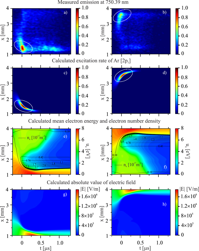
Figure 8. Spatiotemporal variation around breakdown during the first and second half-period of the measured argon emission at 750.39 nm (a) and (b), the calculated excitation rate of Ar[2p1] atoms in all electron-impact excitation processes (c) and (d), the calculated mean energy and number density of electrons (e) and (f), the calculated electric field (g) and (h) obtained in the stable state of the discharge at p = 300 mbar, U0 = 1.5 kV and f = 24 kHz. The values of the measured emission and calculated rate are normalised with respect to their maximum values.
Download figure:
Standard image High-resolution imageFrom the PROES measurement results, regions with the highest light emission can be observed at the moment of the gas breakdown in front of the momentary cathode (figures 8(a) and (b)). These regions are very well reproduced by the calculated excitation rate (figures 8(c) and (d)). This concerns their similar occurrences with respect to time and to the spatial position of the emission maxima. Note that electron-impact excitation of ground state argon atoms to the Ar[2p1] state has the largest contribution to the total production of Ar[2p1] during breakdown. Since the rate of this collision process is determined by the formula k28 ne nAr[1p0], it can be concluded that the good agreement of the measured emission and calculated excitation rate is a further proof of proper spatiotemporal profiles of ne, ue, and E presented in figures 8(e)–(h).
Thus, we can summaries that the proposed 23-species RKM reproduces the plasma behaviour very well at the investigated conditions and that it can be used for different analyses of DBDs in argon plasmas.
4.2. Test case 2
The measured data used for this further evaluation of the 23-species RKM was obtained for an atmospheric-pressure DBD, which has previously proven as suitable for the analysis of the thin-film deposition in mixture of argon with small amounts of HMDSO or TMS [40–42]. The plane-parallel discharge configuration with rectangular steel mesh electrodes is 10 mm long (in gas flow direction) and 80 mm wide. Thus, the discharge area is A = 8 cm2. Dielectric layers made of borofloat glass with a thickness Δ of 2 mm are glued onto the electrodes. The gas gap d is 1 mm. The purity of argon gas used in the experiment was 99.9999% (Ar 6.0) [40]. The discharges were driven by a sinusoidal voltage provided by a high-voltage generator (G2000, Redline Technologies, Baesweiler, Germany) and the gas flow rate was 6 slm. A sketch of the plasma source is given in figure 1(a) and the discharge parameters are listed in table 4.
Two independent approaches were used to measure the discharge current as described in [42]. In the first case, the grounded electrode was connected in series to a 1 Ω precision resistor R and the voltage UR measured across the resistor was used to determine the discharge current Iexp, R(t) = UR(t)/R. In the second case, a capacitor C with a capacitance of 32.5 nF was placed instead of the resistor. The measured transferred charge Q(t) was used for the determination of the current Iexp, C(t) = dQ(t)/dt. All measured signals were monitored by a digital oscilloscope (MDO3052, Tektronix, Beaverton, OR, USA, 500 MHz bandwidth).
In order to analyse the described plasma source by means of the fluid-Poisson model, the same finite-difference method as used in [37, 72] was applied to solve the set of equations (2)–(7). In case of the balance equations of charged particles and mean electron energy, the exponential scheme based on Scharfetter and Gummel [90] was used for the spatial discretisation. The central-difference method [91] was applied for the solution of Poisson's equation and the balance equations of metastable argon atoms. The calculation domain was divided into 500 non-equidistant spatial intervals, logarithmically refined towards the boundaries. The time step size was automatically adapted to keep the relative error of the mean electron energy below the tolerance of 10−4. The same initial conditions as in section 4.1 were used.
Figure 9 shows the comparison of the calculated discharge currents using the 15-species and 23-species RKM and measured data during one voltage period in the stable periodic state of the discharge. The measured current signals Iexp, R(t) and Iexp, C(t) agree very well, which proves the reliability of the measurements. The current peaks representing the breakdown of the discharge are visible in the results of both models. However, the instants of the breakdown events predicted by the two models are different. In case of the 23-species RKM, the moment of the occurrence of the current peaks is in good agreement with the experimental data. The intensity of the calculated current peak around t = 3 μs also agrees well with measured currents and the agreement around t = 9 μs is satisfactory.
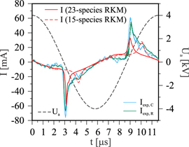
Figure 9. Comparison of the measured (Iexp, C and Iexp, R) and calculated (I ) discharge currents using the 15-species and 23-species RKM in the periodic state of the atmospheric-pressure DBD analysed in [40–42] at U0 = 4 kV and f = 86.2 kHz (T = 11.6 μs). Zero value of the time axis corresponds to t = 84.1 μs (7.25T ).
Download figure:
Standard image High-resolution imageThe results obtained by use of the 15-species RKM show a delayed breakdown compared to the experimental and the calculated 23-species RKM results. It is found again that the electron energy loss due to electron-impact excitation processes of ground state argon atoms resulting from the 15-species RKM is larger than in the case of the 23-species RKM. Thus, the mean electron energy obtained using the 15-species RKM is smaller, which leads to a lower electron production due to electron-impact ionisation processes. This implies that more time is needed to meet the breakdown condition when using the 15-species RKM and explains the delayed breakdown compared to the 23-species RKM.
The corresponding temporal evolution of the spatially averaged electron number density  as well as the discharge current I obtained by model calculations is represented in figure 10. It is found that
  obtained by use of the 15-species RKM is mostly lower than that predicted by the 23-species RKM. The larger electron number density of the 23-species RKM at the moment of gas breakdown leads to higher absolute values of the current peaks. Furthermore, the results of the 23-species RKM demonstrate that the current peaks in the two half-periods have different absolute values. This behaviour of the discharge current agrees with the measured data (figure 9). It is affected by a different temporal evolution of
  in the two half-periods (figure 10(a)). The results obtained using the 15-species RKM do not show this feature of I (figure 10(b)). Here, both current peaks have almost equal intensities.
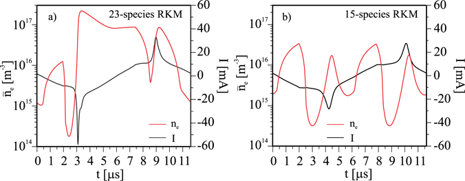
Figure 10. Periodic behaviour of the spatially averaged electron number density  and the discharge current I determined by use of the 23-species (a) and 15-species (b) RKM at the conditions in figure 9.
Download figure:
Standard image High-resolution imageThe asymmetric behaviour of I(t) is strongly connected with an asymmetric spatiotemporal evolution of the electron number density ne(x, t) as shown in figure 11. Here, every breakdown event is highly influenced by the previous one, which indicates that memory effects are responsible for the observed asymmetric discharge behaviour.

Figure 11. Spatiotemporal variation of the electron number density ne(x, t) and temporal evolution of the discharge current I(t) in the first seven voltage periods at U0 = 4 kV, f = 86.2 kHz and p = 1 atm obtained by use of the 23-species RKM.
Download figure:
Standard image High-resolution imageThe reproduction of the temporal evolution of a measured current is quite difficult, regardless of the type of the model. Based on the analysis for test case 2 it can be said that good agreement between calculated and measured discharge currents substantiates that the 23-species RKM can also be used well for investigations of DBDs at atmospheric pressure.
4.3. Test case 3
The third test case of the proposed 23-species RKM is performed for a megahertz-driven μAPPJ. This plasma source consists of two parallel stainless steel electrodes covered with quartz glass windows that allow access for optical measurements. The electrodes are 20 mm long and 1 mm wide resulting in a discharge area A of 20 mm2. The gap d is 1.3 mm so that the embedded discharge channel has the volume V = 26 mm3. Argon gas with the same purity level as in the first test case (99.999%) was used here [86]. A function generator (AFG3252, Tektronix) was used to power the discharge with a sinusoidal voltage. A schematic representation of the plasma source is shown in figure 1(b) and the discharge parameters are listed in table 4.
PROES measurements of the spatiotemporal evolution of the plasma emission at 811.53 nm are conducted similarly as in the first test case (section 4.1) with the aid of a high-repetition rate-gated iCCD camera (PicoStar HR12, LaVision GmgH, Germany). Further details about the experimental setup and measurement procedures can be found in [38].
The discharge generated in the plasma jet under the investigated conditions represents an atmospheric-pressure RF glow discharge. This discharge can be operated in two different modes. In the α-mode, the electron production is mainly determined by bulk ionisation, while secondary electrons generated at the cathode surface are the main channel of electron production in the γ-mode [38]. For the numerical modelling of discharges in these two modes and in the α–γ transition regime, the measured dissipated power was used as input. In each period the applied voltage amplitude U0 was automatically adapted by the relation

until reaching periodic state. Here, Pexp denotes the measured power and Pcalc is the calculated current averaged power. The constant c has been taken to be 0.25 in accordance with [38]. The use of this procedure ensures that Pexp and Pcalc have the same values when the periodic state of the discharge is reached. A similar numerical procedure as in the second test case (section 4.2) was used to solve the fluid-Poisson model. Details about the used initial and boundary conditions are given in [38].
The experimental studies of the μAPPJ reported in [38] were supplemented by time-dependent, spatially one-dimensional fluid model calculations using the 15-species RKM. The results of PROES measurements for the emission line at 750.39 nm (Ar[2p1] → Ar[1s2] transition) at the dissipated power of 0.6 and 1.3 W, respectively, were compared with the calculated ground state excitation rate of the lumped Ar[2p'] state comprising the states 2p4–2p1. At the powers used in the experimental studies, the discharges operate in the α-mode and in the transition regime from α-mode to γ-mode, respectively. To reproduce these discharge modes, the applied power in the model calculations was chosen to be 1.4 and 3.0 W, respectively. Since the argon emission at 750.39 nm is mainly caused by direct electron-impact excitation of Ar[1p0], the comparison became possible and showed very good agreement.
A corresponding analysis was also performed for the emission at 811.53 nm determined by the radiative transition Ar[2p9] → Ar[1s5]. The measured data were compared with the calculated total excitation rate of the lumped Ar[2p] state comprising the states 2p10–2p5. This excitation rate includes ground state and stepwise excitation due to electron collisions. Opposite to the comparison for the emission line at 750.39 nm, certain differences between measured and calculated results were found.
The proposed 23-species RKM includes all individual 2p states, i.e. a direct comparison with the PROES results for the emissions at 750.39 nm and 811.53 nm becomes possible. The results of model calculations using the 23-species RKM show that the main contribution to the emission at 750.39 nm comes from direct electron-impact excitation of Ar[1p0]. Generally, the modelling results show good agreement with the measured emission at 750.39 nm, similar to the results obtained by use of the 15-species RKM shown in [38]. Therefore the focus of the analysis is on the emission at 811.53 nm.
Figure 12 shows corresponding results related to the emission at 811.53 nm, where the applied power of 0.6 and 1.3 W was used for the modelling studies using the 23-species RKM, in accordance with the measurements. The figure includes the periodic behaviour of the calculated discharge voltage and current as well as the spatiotemporal behaviour of the measured argon emission, the calculated production rate of the Ar[2p9] state due to all electron-impact excitation processes and the calculated mean electron energy ue(x, t). Notice that the measured emission and calculated excitation rates are normalised with respect to their maximum values at higher power for direct comparison.

Figure 12. Periodic behaviour of the calculated discharge voltage and current (a) and (b) and spatiotemporal variation of the measured argon emission at 811.53 nm (c) and (d), the calculated excitation rate of Ar[2p9] atoms in all electron-impact excitation processes (e) and (f) and calculated mean electron energy (g) and (h) at the power of 0.6 and 1.3 W, respectively, and the frequency of 27.12 MHz (T = 36.9 ns). The values of the measured emission and calculated excitation rates are normalised with respect to their maximum values at higher power. Zero value of the time axis corresponds to t = 88.6 μs (≈2400T ).
Download figure:
Standard image High-resolution image
As expected, the results for the discharge voltage and current (figures 12(a) and (b)) show larger values at higher applied power. The electrical properties can be related to the emission intensity as well as patterns measured by PROES. When analysing the results of the PROES measurements at 811.53 nm (figures 12(c) and (d)), two maxima labelled as I and II can be clearly noticed. Although the emission at lower power (0.6 W) is much weaker than at higher power (1.3 W), the same emission pattern can be identified. When comparing these results with the calculated total electron-impact excitation rates of Ar[2p9] (figures 12(e) and (f)), very good agreement is found for both applied powers. The same emission maxima are reproduced by the model calculations. Especially, their occurrence in time corresponding to the maximum current magnitude as well as their positions in space are reproduced convincingly. Their existence can be explained by the spatiotemporal evolution of the mean electron energy. It can be seen that the maximum values of the calculated production rate (figures 12(e) and (f)) correspond to the maximum electron energy of bulk electrons (figures 12(g) and (h)) indicating that the bulk electrons are responsible for the excitation. The analysis of the individual electron-impact excitation rates of Ar[2p9] shows that ground state excitation is the predominant process followed by the excitation of Ar[1s5]. Note that for the investigated conditions, secondary electrons accelerated by the strong electric field in front of the momentary cathode have the highest mean energy in the gap, but a small contribution to the total Ar[2p9] production due to the low number density of electrons in this region.
It turns out that the influence of secondary electrons on the plasma behaviour cannot be studied from the emission at 811.53 nm, as it was the case for the emission at 750.39 nm [38]. Based on this analysis, it can be concluded that the proposed 23-species RKM provides the possibility to understand the plasma behaviour not only in DBDs, but also in other types of gas discharges, such as the μAPPJ configuration with plane electrodes.
5. Conclusions
A 23-species RKM for the analysis of weakly ionised, non-thermal argon plasmas with gas temperatures around 300 K at sub-atmospheric and atmospheric pressures is presented and discussed. In addition to electrons, it takes into account the ground state atom, 15 excited atomic and four excited molecular states as well as the atomic and molecular ion of argon. In particular, the four individual 1s and the ten individual 2p excited states are considered as separate species. This RKM includes 409 collision processes and radiative transitions as well as recent data on electron collision cross sections. It has been successfully applied in the framework of time-dependent, spatially one-dimensional fluid modelling of three test cases involving two DBD configurations at atmospheric and lower pressure with different applied voltages, frequencies and setups as well as a megahertz-driven atmospheric-pressure plasma jet.
The comparison of modelling results and experimental data includes measurements of the discharge current, of the absolute number density of Ar[1s5] atoms determined by means of LAAS and different emission lines applying PROES. Generally good agreement between measured and calculated data has been found.
The comparison with results obtained by use of a previously established 15-species RKM using former electron collision cross section data illustrates the wider applicability of the proposed 23-species RKM and demonstrates partly better agreement of the 23-species RKM results with measured data. Thus, the proposed 23-species RKM can be used as a helpful tool for further, more detailed analysis. A final estimation of its applicability requires a broader and more systematic comparison with experimental data, including further plasma sources operating over a wide range of discharge properties. This will be part of future studies.
Acknowledgments
This work was partly funded by the Deutsche Forschungsgemeinschaft (DFG, German Research Foundation)—Project Number 368502453, Project CEPLANT (LM2018097) funded by the Ministry of Education, Youth and Sports of the Czech Republic and Project No. 21-16391S funded by the Czech Science Foundation. The authors also thank R Bansemer, A K Czerny, H Höft and C-P Klages for providing experimental data and helpful discussions related to the experimental investigations. Furthermore, the authors are grateful to K Bartschat and O Zatsarinny for providing additional electron-impact excitation cross sections of Ar[1s5...2].
Data availability statement
The data that support the findings of this study are openly available at the following URL/DOI: https://doi.org/10.34711/inptdat.585 [92].