
Abstract
This is the second part of a set of two papers on radio-frequency (RF) discharges, part of a larger series on the foundations of plasma and discharge physics. In the first paper (Chabert et al 2021 Plasma Sources Sci. Technol. 30 024001) the two basic configurations of RF discharges commonly used in industrial applications, the capacitive and the inductive discharges, are presented. The introduction of an external magnetic field to these discharges results in not only a quantitative enhancement of their capabilities but also leads to qualitatively different interaction mechanisms between the RF field and the plasma. This provides rich opportunities for sustaining dense plasmas with high degrees of ionization. On one hand, the magnetic field influences significantly the particle and energy transport, thus providing new possibilities for control and adjustment of the plasma parameters and opening even lower operation pressure windows. On the other hand, when the magnetic field is introduced also in the region where the plasma interacts with the RF field, qualitatively new phenomena arise, that fundamentally change the mechanisms of power coupling to the plasma—the electromagnetic energy can be transported as waves deeper into the plasma volume and/or collisionlessly absorbed there by wave resonances. The characteristics of these discharges are then substantially different from the ones of the standard non-magnetized RF discharges. This paper introduces the physical phenomena needed for understanding these plasmas, as well as presents the discharge configurations most commonly used in applications and research. Firstly, the transport of particles and energy as well as the theory of waves in magnetized plasmas are briefly presented together with some applications for diagnostic purposes. Based on that the leading principles of RF heating in a magnetic field are introduced. The operation and the applications of various discharges using these principles (RF magnetron, helicon, electron cyclotron resonance and neutral loop discharges) are presented. The influence of a static magnetic field on standard capacitive and inductive discharges is also briefly presented and discussed.
Export citation and abstract BibTeX RIS

Original content from this work may be used under the terms of the Creative Commons Attribution 4.0 licence. Any further distribution of this work must maintain attribution to the author(s) and the title of the work, journal citation and DOI.
1. Introduction
Magnetized discharges, i.e. discharges with an applied external magnetic field (figure 1), constitute a broad class of plasmas with quite diverse characteristics. The application of a magnetic field not only influences the transport of particles and energy in the discharge, but also opens possibilities for wave and resonant heating of the plasma [1]. Combined with the flexibility of customizing the magnetic field configuration and even adapting it to the changing conditions during plasma processing adds a whole new dimension in the control of the properties of the discharges allowing them to suit various applications. Furthermore, such discharges exhibit a large variety of phenomena that are not present in their non-magnetized counterparts such as drifts, waves and resonances, discharge anisotropy and instabilities [2]. This provides rich field for fundamental research as well, although at the expense of making it also more challenging to explore.
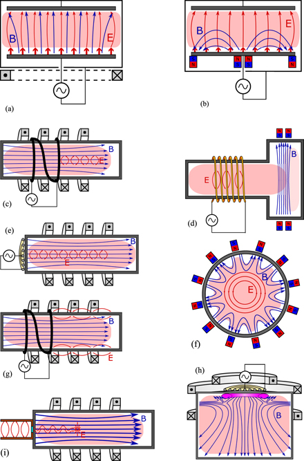
Figure 1. Schematic representation of the various types of magnetized RF discharges: (a) a capacitive discharge with a longitudinal magnetic field, (b) a capacitive discharge with a transverse magnetic field (RF magnetron), (c) inductive discharge with a longitudinal magnetic field (helicon-type discharge), (d) inductive discharge with a transverse field, (e) helicon discharge with a flat coil, (f) inductive discharge with a multi-cusp confining field, (g) discharge with Trivelpiece–Gould mode, (h) neutral loop discharge, (i) electron cyclotron resonance discharge. The force lines of the static magnetic field and of the RF electric field are also shown in blue and red, respectively.
Download figure:
Standard image High-resolution imageIn the industrial application of radio-frequency (RF) discharges, e.g. capacitive and inductive discharges, the addition of an external magnetic field provides possibilities for tailoring the plasma performance beyond what is possible by the standard means [3] (variation of the pressure, power and RF frequency). The enhanced plasma confinement due to the magnetic field leads to an increase of the plasma density and thus reaching ionization degrees close to 100% becomes possible. This in turn improves the processing rates, which is always desired. The beauty of magnetized plasmas is also their ability to exploit resonances rather directly and benefit from this efficient mechanism for energy coupling.
One should then think that all commercially used plasmas nowadays are magnetized. However, this is not the case since creating homogeneous magnetic fields over large areas is very difficult and costly. The resonance condition, providing the efficient energy coupling, is usually only fulfilled in a small spatial region leading to narrow processing windows and very inhomogeneous plasmas. Nevertheless, magnetized plasmas still find their place in industrial applications, albeit usually quite limited. However, these magnetized plasmas really flourish in applications which are rather specific and typically in fields that are emerging only in recent years such as thrusters, plasma accelerators or small ion sources.
The influence of a magnetic field on the transport is used in multi-cusp sources (figure 1(f)) to reduce the particle losses to the walls, thereby enhancing the plasma density and improving the plasma uniformity. Such sources are applied in situations where dense plasmas at low pressures are required. RF magnetrons (figure 1(b)) are another important class of discharges with magnetic confinement of the electrons designed to prevent them from reaching the RF biased electrode. Here a cusp magnetic field configuration traps the electrons in a region in front of the sputtering target. This creates a dense plasma that provides large fluxes of energetic ions needed for the sputtering of the target material. If the magnetic field is oriented parallel to the RF electric field (figure 1(a)) then the plasma is prevented from reaching the grounded side walls. This changes the effective size of the grounded electrode and influences the geometrical symmetry of the discharge and consequently changes the self-bias. Recently, in analogy to the electrical asymmetry effect [4, 5], these two situations have been interpreted as magnetic asymmetry [6, 7]. Strong magnetic fields (about 1 T) with such configurations are also used in the field of dusty plasmas [8, 9]. There the magnetic field is intended to magnetize even the heavy dust particles to allow investigations of their behaviour. The physics of the dusty plasmas is beyond the scope of this paper and discharges containing dust particles will not be discussed in the following. The interested reader is directed to e.g. the textbook by Piel [10] and the references therein.
The design of sources of negative hydrogen ions (figure 1(d)) is based on the reduction of the energy transport across the magnetic field lines. In these discharges a magnetic filter field separates the plasma into a region with abundance of energetic electrons and a region of cold electrons [11, 12]. This was envisioned as an enhancement of the volumetric production of negative hydrogen ions through dissociative attachment to vibrationally excited molecules [12]. Magnetic filtering has also been studied in plasma thrusters designed for ion–ion extraction [13, 14].
In magnetized discharges the RF fields can propagate as electromagnetic waves into the plasma bulk well beyond the skin depth that limits the field penetration in classical inductive discharges (ICP). This permits efficient deposition of RF energy in the plasma volume and allows discharges to be sustained with densities much higher than those in ICPs. This is the principle of operation of the helicon discharges (figures 1(c) and (e)), the discharges with Trivelpiece–Gould modes (figure 1(g)) and the neutral loop discharges (figure 1(h)).
The electromagnetic waves exhibit also resonances in magnetized plasmas. In the vicinity of a resonance point the energy of the wave is fully absorbed by the plasma without the need of collisions. This again allows sustaining dense discharges at low gas pressures. Adjusting the field strength provides control over the region where the energy is deposited. Among the most prominent examples here are the electron cyclotron resonance (ECR) sources (figure 1(i)).
The paper is structured as follows. In the beginning, the basic concepts of particle motion and transport in a magnetic field are introduced in section 2. Here, first the cyclotron gyration and the associated quantities (cyclotron frequency, Larmor radius) are derived. Then the single particle drifts are presented, followed by the fluid description of magnetized plasmas. The focus is on the particle and energy transport of electrons in magnetic field. The plasma conductivity and the dielectric tensor are also derived. The description of magnetized plasmas from a kinetic point of view is also briefly introduced. The next section 3 then presents various discharge configurations where external magnetic field is applied for the confinement of the plasma particles and/or of their energy. The first example is the use of longitudinal 3 magnetic field in capacitive discharges for influencing their geometrical symmetry and consequently the self-bias. The RF magnetrons are introduced as a variant of a capacitive discharge with a transverse magnetic field. Next the RF volume sources of negative hydrogen ions are discussed as an example for the use of a magnetic barrier. Finally, inductive discharges with a confining multi-cusp field are introduced. In section 4 the diversity of waves that can propagate in magnetized plasmas is presented. The focus is set on the transverse modes, since they have the biggest relevance both for discharge maintenance and diagnostics. The concepts of cut-off and resonance are introduced. Both cases of unbounded and bounded plasmas are considered and the dispersion relations of undamped waves are presented. Few examples for the use of wave propagation as a diagnostic tool are also presented. The relations obtained in section 4 are then used in section 5 to describe the physics of the helicon plasma sources. The damping mechanism and the radial structure of the discharge are discussed. The Trivelpiece–Gould mode discharges are mentioned in passing as a subbranch of this type of discharges. The antenna designs and the different regimes of helicon discharges (E, H, W) are presented. Finally, the neutral loop discharge is introduced as a special case of the helicon plasma source. The paper closes with the introduction in section 6 of the sources that use ECR for sustaining the discharge. Their principles of operation are discussed and the energy gain under resonance conditions is presented. The advantages and disadvantages of these sources are briefly presented. The various application fields for these discharges are summarized, followed by the conclusions.
2. Plasma behaviour in a static magnetic field
2.1. General scalings
In a magnetic field B the charged particles with a charge q and a mass m moving at a velocity  exhibit an additional force
  . This is known as the Lorentz part of the electro-magnetic force
  , where
  is the electric field. Under the influence of this additional force the particles gyrate with the cyclotron frequency
4
defined as ωc = |q|B/m [15]. The radius of the gyro-motion, known as the Larmor radius, is determined by the perpendicular component v⊥ of the particle velocity: rL = mv⊥/|q|B = v⊥/ωc. These quantities are among the important parameters that characterize the influence of the magnetic field on the discharge behaviour. The cyclotron frequency for electrons and ions with mass mi is, respectively,
is the electric field. Under the influence of this additional force the particles gyrate with the cyclotron frequency
4
defined as ωc = |q|B/m [15]. The radius of the gyro-motion, known as the Larmor radius, is determined by the perpendicular component v⊥ of the particle velocity: rL = mv⊥/|q|B = v⊥/ωc. These quantities are among the important parameters that characterize the influence of the magnetic field on the discharge behaviour. The cyclotron frequency for electrons and ions with mass mi is, respectively,

where mp is the proton mass. In laboratory plasmas the typical magnetic field strengths are in the range of B = 10 mT or less, although in individual cases, e.g. in linear machines or in ECR sources, also an order of magnitude higher values are possible. Then the cyclotron frequency of the electrons is of the order of fc e = ωc e/2π = 280 MHz and of the protons fc p = 150 kHz. For heavier ions the cyclotron frequency is even lower. This means that for the typical RF frequencies ω/2π in the range 10 MHz–100 MHz the following inequalities are usually well satisfied ωc i ≪ ω ≪ ωc e. The Larmor radius can be estimated using the characteristic velocities of the particles. For the electrons this is their thermal velocity  106 m s−1 and for the ions this is the Bohm velocity uB ∼ 103 m s−1. Then rL e ∼ 0.6 mm for the electrons and rL i ⩾ 10 mm for the hydrogen ions. Useful expressions for the estimation of the Larmor radii for electrons and ions with the kinetic energy ɛ are:
The most prominent effect of the magnetic field is the reduction of the particle and energy transport perpendicular to the field lines. As will be shown later (see equations (33) and (49)), in the DC case the perpendicular mobility μ⊥, diffusion coefficient D⊥ and thermal conductivity coefficient χ⊥ are all reduced by a factor of  , with νm and λm the collision frequency and the mean free path for momentum relaxation, respectively. The transport parallel to the field lines is not affected. Obviously, the effect of the magnetic field is significant when ωc ⩾ νm or rL ⩽ λm, i.e. at low pressures and/or large magnetic field strengths.
For the majority of gases at a pressure p the elastic collision frequencies for momentum exchange of the electrons and the ions with the background gas, νm e and νm i, can be roughly estimated by

Therefore, for the electrons to be magnetized (ωc e > νm e), the magnetic field strength has to exceed B/T > 1 × 10⁻⁴(p/Pa) while to magnetize the ions, a field strength of B/T > 1 × 10⁻³(mi/mp)(p/Pa) is needed. Note that these values are not exact and have to be adjusted for the particular situation at hand. Still, it becomes evident, that even relatively weak magnetic fields of the order of 1 mT are sufficient to magnetize the plasma at low pressures (p ∼ 1 Pa), whereas for atmospheric pressure discharges the effects of the magnetic field can be mostly ignored. The above estimations also show that the laboratory magnetic fields are much more important for the behaviour of the electrons than for that of the ions. Consequently, the energy coupling and the transport of the electrons are strongly influenced, while the heavy ions are mostly unaffected and the magnetic field is usually neglected for their description.
2.2. Cyclotron gyration and drifts
To quantify the effects of a magnetic field we will first discuss its influence on the motion of individual charged particles. Their behaviour in a static magnetic field  under the action of an external force
  is described by the equation of motion:

Due to the cross product the magnetic field influences only the particle motion perpendicular to the field lines. Note that the effect of an electric field  is a special case of this generalized treatment when
  . Multiplying by

it becomes evident that the change in the kinetic energy is determined only by the work W done by the force  per unit time, i.e. by its power
  , while the magnetic field conserves the energy of the particle.
Taking the time derivative of the equation of motion (4) results in:

Here it has been assumed that the force can depend only on time but not on space. This treatment can easily be extended to the case with spatial gradients of the electric field. The magnetic field on the other hand can vary only in space but not in time. The externally applied magnetic fields are usually static or quasi-static, i.e. their temporal variation is slow compared to the changes in the velocity. Fast changing magnetic fields, e.g. those in electromagnetic waves, lead to non-linear phenomena such as the ponderomotive force [3] and generally have negligible effects in gas discharges. The derivative  describes the change in the magnetic field that the particle 'sees' while moving along its trajectory. Substituting the acceleration
  on the right from expression (4) and rearranging one obtains:

The parallel part of this equation is trivial since it does not involve the magnetic field. This can be seen already from equation (4). For further analysis we will concentrate on the part of this vector equation that is perpendicular to the magnetic field, for which the subscript ⊥ will be used. The perpendicular part reads:

where the following notation has been introduced  with:
with:


When  , i.e. when the velocity
  changes little over the cyclotron period, equation (8) has a simple solution:

The first term describes the cyclotron gyration with a frequency ωc around a point called the guiding centre. The sign in the second component of the term depends on the sign of the particle charge and describes the direction of gyration. The rule is that the circular current, resulting from the particle gyration, induces a magnetic field that tries to compensate the external field causing the gyration. Therefore, the plasmas exhibit diamagnetic properties—the external magnetic field is weakened inside the plasma. Looking along the magnetic field lines in the direction of the field, the electrons rotate clockwise following the rule of the right-hand and the positive ions rotate counter-clockwise following the rule of the left-hand (figure 2).

Figure 2. Direction of the gyro-motion of positive and negative charges. The rule of the left and of the right-hand are also illustrated.
Download figure:
Standard image High-resolution imageIntegrating the first term in time again provides the equation for the particle trajectory in static, homogeneous magnetic field:

The trajectory is a circle with a radius rL = v⊥,0/ωc called the Larmor radius of the particle. The rotation is around a point in space called guiding centre. Its position is given by the vector  that is determined by the initial position of the particle.
The second term in equation (12) describes the slow (over many cyclotron periods) motion of the guiding centre in a direction perpendicular to the magnetic field, i.e.  is no longer a constant but depends on time. This process is called 'drift' and equations (9)–(11) give the various types of drifts [16]. The general mechanism behind the drift motion is a small, gradual and periodic change in the Larmor radius throughout the cyclotron motion. This effect is treated as a perturbation to the cyclotron motion and leads to a slow (compared to the gyration period) shift of the guiding centre (figure 3). One of the possible reasons for this gradual change in the gyro-radius is a force that periodically accelerates and decelerates the particle along its orbit. The other possibility is a change in the magnetic field, that entails a change in the Larmor radius. Based on the underlying mechanisms and the nature of the force, various drift motions are possible.

Figure 3. Illustration of the mechanism of the drift motion. The Larmor radius  in the upper half cycle of the gyro-motion is slightly larger than the Larmor radius rL during the lower half cycle, causing a slight shift in the position of the guiding centre (central dot). The movement of the guiding centre with a velocity vd then results in a trajectory similar to the one on the right (the horizontal shift has been significantly exaggerated for clarity).
Download figure:
Standard image High-resolution imageThe simplest form of a drift is the one under the influence of an external force acting perpendicular to the magnetic field. It is described by a motion of the guiding centre with a velocity  that is perpendicular both to the magnetic field and the force (equation (10)). The force accelerates the particle during one half-period and decelerates it during the second half, causing the change in the gyro-radius that leads to the drift. A particular case is the E × B-drift under the influence of the electric force
  [2, 15]:

The direction of this drift does not depend on the charge or the mass of the particles. Therefore, both electrons and ions are drifting in the same direction with the same velocity and the drift motion does not lead to a net current. In many instances only the electrons are drifting, while the ions are only weakly magnetized. In this case, a current due to the E × B drift actually flows.
The polarisation drift (equation (9)) appears under the influence of a slow time variation in the force, e.g. in time-varying electric fields:

The drift occurs because the acceleration phase is slightly different than the deceleration phase due to the small change in the force within the cyclotron period. Under such conditions a polarisation current arises [2]:

Note that when the rate of change in the electric field is comparable to the period of the gyro-motion the term can no longer be separated from the cyclotron motion, i.e. it is no longer a small perturbation. In the case when  (plus sign for the ions) it leads to the cyclotron resonance heating (v⊥ increases linearly in time, see section 6 below).
The last drift motion (equation (11)) describes drifts due to inhomogeneities in the magnetic field. To derive the explicit form of these drifts the magnetic field is expanded in the vicinity of the guiding centre:

and then expression (11) is averaged over the cyclotron period after replacing the velocity with the first term in equation (12). The two typical examples that result from this treatment are the ∇B drift due to a change in the magnetic field strength in the perpendicular direction  and the centrifugal drift due to curvature in the magnetic field lines. These drifts are given as [1, 2]:

and (Rc is the radius of the curvature)

Often they are combined together into a single expression.
In an inhomogeneous magnetic field, the two components of the velocity,  and
and  , are coupled to each other. This follows from the conservation of the energy and the magnetic flux enclosed by the particle gyro-orbit. Traditionally, the latter is written in terms of the first magnetic invariant μ, defined as [2]:

This definition is identical to the definition of the magnetic moment of a current loop that is created by the gyration of the charged particle. The magnetic flux through this loop is:

It can be shown (see e.g. [2]) that μ and hence also Φ are conserved during the particle motion along the magnetic field lines. This implies that when the magnitude of the external field B0 increases, so does the perpendicular velocity of the particles. Since the magnetic field conserves the kinetic energy of the particles, this entails that the velocity along the magnetic field line v|| has to decrease. Eventually v|| can become zero at which point the particle is reflected back towards the region of weaker magnetic field. This principle lies in the basis of the magnetic mirrors. It is also part of the mechanism for plasma confinement by multi-cusp magnetic configuration (section 3.2).
2.3. Particle transport in a static magnetic field
The influence of the magnetic field on the motion of individual particles is also seen in their collective behaviour. This behaviour is described by the macroscopic quantities (moments of the distribution function)—particle density n, fluid flow velocity  , energy flux density
  , etc. These parameters are determined by the corresponding fluid equations. The magnetic field does not enter in the equations for the scalar fluid moments (particle and energy balance), but appears in the ones for the vector (flux) quantities—momentum and energy flux of the particles. Therefore, the magnetic field affects the plasma by influencing the transport of particles and energy. In the following we will concentrate on the electrons since they experience the effects both of the magnetic field and of the RF electric field more strongly than the ions. However, most of the obtained relations can be easily applied also for the ions. For brevity we will be omitting the index 'e'. Further, the relations in this section pertain only to the case of relatively weak magnetic fields (ωc < ωp, with ωp the plasma frequency) when the effect of the magnetic field on the collisions can be neglected. For the opposite case of strongly magnetized plasmas when the electron cyclotron radius becomes smaller than the Debye length, the reader is redirected to [17] and the references therein.
The transport of electrons is described by their momentum balance. In a static magnetic field  it takes the form

where the electric field  can vary in space and time. Here the non-linear convective term
  has been neglected, since the treatment will be restricted only to the linear effects. The description of phenomena based on non-linear interactions generally requires a more involved treatment that goes beyond the scope of the present article. The electron pressure is assumed to be isotropic, i.e. it is represented by the scalar pressure p = nkB
T with kB the Boltzmann constant and T the electron temperature. This requires that the electron velocity distribution function is isotropic:
has been neglected, since the treatment will be restricted only to the linear effects. The description of phenomena based on non-linear interactions generally requires a more involved treatment that goes beyond the scope of the present article. The electron pressure is assumed to be isotropic, i.e. it is represented by the scalar pressure p = nkB
T with kB the Boltzmann constant and T the electron temperature. This requires that the electron velocity distribution function is isotropic:  , i.e. it does not depend on the direction of the electron velocity
  . Note, that in magnetized plasmas this is generally not guaranteed. In this case the electron pressure has to be treated as a tensor, i.e. the pressures along and perpendicular to the magnetic field lines are not necessarily the same (p|| ≠ p⊥). Then the gradient of the pressure has to be replaced by the divergence of the pressure tensor
  where the latter is given by

when the magnetic field is directed along the third axis. The two components of the pressure are determined by two temperatures: p||,⊥ = nkB T||,⊥. The mean energy of the electrons is then ⟨ɛ⟩ = kB T⊥ + kB T||/2 (two degrees of freedom for the perpendicular and one for the parallel motion).
Replacing the derivative in time in equation (22) with iω 5 , i.e. performing a Fourier transform in the time domain, and after some manipulation the following expression for the electron flow velocity can be obtained [18]:

with

When discussing quasi-stationary transport, e.g. deriving the ambipolar diffusion, the limit ω → 0 is taken and then Ω = ωc/νm. For the treatment of undamped wave propagation the limit νm → 0 is considered resulting in Ω = −iωc/ω. When the frequency of the field oscillation approaches the cyclotron frequency, care has to be taken in the treatment since the term  diverges in the collisionless case.
The tensor

is characteristic for the transport properties in magnetized plasmas. As it will become evident, it appears also in the expression for the energy flux as well as in the kinetic description. It is also related to the conductivity and the dielectric tensor of the plasma (equations (53) and (54)). In a Cartesian coordinate system, in which the magnetic field is along the third axis, it is represented by the matrix:

The first two diagonal elements, arising from the unit tensor  , describe the transport perpendicular to the magnetic field. The third diagonal element results from the combination of the first two tensors in (27) (
 is the dyadic product) and gives the transport along the field. The off-diagonal elements come from the cross product term and represent the drifts. With this tensor, equation (24) can be rewritten in a form similar to the non-magnetized case:

The mobility and diffusion tensors are expressed by the tensor  (equation (27)):

and
The parallel components of these tensors coincide with the usual expressions in non-magnetized discharges (μ and D, respectively):

In magnetized plasmas usually only the static (ω = 0) transport is considered and the expressions become:

The perpendicular components are thus reduced by the magnetic field by a factor  :
:

It becomes evident that at high pressures, i.e. high collisionality (ωc ≪ νm) the effect of the magnetic field is diminished while for strong magnetic fields the transport coefficients are strongly suppressed. The off-diagonal components describing the drifts are

These terms describe transport perpendicularly to the applied forces and are a consequence of the magnetic field. In case of strong collisions (ωc ≪ νm) they vanish.
To aid the understanding of the meaning of the off-diagonal elements, they can be written out separately in equation (28). Then from the mobility term one obtains the E × B drift (equation (14)), scaled by  . The diffusion term produces the diamagnetic drift:

also scaled by the same factor. The diamagnetic drift is a pure collective effect and does not appear in the single particle description [2, section 3.4].
With the mobility μ⊥ and the diffusion coefficient D⊥ given by equation (33) the coefficient for ambipolar diffusion perpendicular to the magnetic field can be derived in the usual way. The result is:

where the indices e and i pertain to the electrons and the ions, respectively. Due to the stronger influence of the magnetic field on the electrons, in magnetized plasmas the mobility of the ions can be higher than that of the electrons. Then for the usual case of cold ions (Ti ≪ Te), D⊥a ≈ D⊥e, i.e. the plasma is diffusing to the walls with the diffusion constant of the electrons. However, the electron diffusion is much slower (better plasma confinement) due to the reduction of the electron transport by the magnetic field by the factor  . Then the particle loss rate also scales as
  . However, in strongly magnetized discharges it was observed that the actual diffusion constant is better described by [19]

This is called Bohm diffusion after David Bohm, the first to describe it [20]. The qualitative explanation involves E × B-drifts in turbulent electric fields caused by plasma instabilities [20, 21]. The weakening of the magnetic confinement by turbulence fluctuations has been observed in numerical simulations [22]. However, the numerical factor in (37) is just an empirical value and has no theoretical explanation. It can also slightly vary between the different experiments.
For magnetized plasmas contained in vessels with conducting walls sometimes also another form of diffusion is possible. It is termed Simon diffusion after the person who has first derived the transport coefficients. They differ from expression (36) [23–26]. In this case the ion flux perpendicular to the magnetic field is much larger than the electron flux due to the strongly reduced transport coefficients of the electrons. The electrons then leave the plasma mainly in the direction parallel to the field lines (figure 4). This imbalance of the particle fluxes leads to electrical current that closes along the conducting walls of the plasma vessel. Naturally, this is only possible, if the transport of the electrons along the magnetic field lines is more efficient than that across them. This aspect has been demonstrated by simulations in [27]. The transition between the two limiting cases is studied by Fruchtman [28].
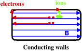
Figure 4. Illustration of the principle of Simon diffusion.
Download figure:
Standard image High-resolution imageThe fluid equations presented above provide correct description only for the ensemble of particles. However, the ensemble-averaged coefficients in those equations, e.g. the collision rates, cannot be calculated within the fluid description and require external information in the form of a particle distribution function. Usually either an assumption for the type of the distribution function is made or some simplified version of a kinetic treatment is invoked. Furthermore, the obtained quantities depend on the stage at which the ensemble average is carried out. This can lead to results for the transport coefficients that differ from the ones obtained via (29) and (30). Furthermore, stochastic effects, like e.g. wave–particle interactions cannot be described within the fluid picture. To capture such effects, one needs to turn to kinetic description.
For obtaining the kinetic counterparts of the transport coefficients (29) and (30), the two-term approximation for the distribution function [29] is used. The essential aspect here is that in magnetized plasmas the anisotropic deviations from the equilibrium distribution f0(v) appear in all three directions and can be different, i.e. the second term in the expansion of the distribution function  is a vector-valued function
  [18]:
[18]:

The anisotropic part is obtained as a solution to the following vector equation:

where the electric field can vary both in space and time. Note that here the elastic collision frequency can depend on the velocity:  , with Ng the density of the neutral atoms and
  the cross section for momentum exchange in elastic collisions with the neutrals. Equation (39) is obtained as an average of the Boltzmann equation over the solid angle in velocity space. The major approximations are related to the treatment of the collisional integrals. Consequently, this equation, and the two-term approximation in general, as well as the results obtained within the approximation allow capturing of all non-local stochastic effects contained also in the collisionless Boltzmann equation. However, the structure of the approximation, i.e. the decomposition of the distribution function, is not particularly well suited for that (both f0 and f1 can vary in space and time), especially in magnetized plasmas. Therefore, perturbative approaches are preferred instead and are practically the standard for dealing with non-local effects. One has to also point out that the magnetic field actually reduces the extent of the non-local effects since it binds the particles to the field lines and limits their movement along possible spatial gradients.
The structure of (39) is identical to the one of equation (22) and, consequently, the solution has a very similar form:

In obtaining this expression again only the stationary situation is considered and hence Ω(v) = ωc/νm(v). Inserting this result into the expression for the velocity:

provides a relation similar in structure to equation (28). Through comparison of the corresponding terms, the kinetic expressions for the mobility and the diffusion coefficient are obtained:


In the last step it has been assumed that  . For this condition to be satisfied, it is sufficient that the magnetic field and the gas density do not vary in space. Then

Similarly to the non-magnetized case, the kinetic treatment results in the diffusion coefficient appearing under the spatial derivative. Further, the kinetic mobility and diffusion coefficients coincide with their fluid counterparts when the collision frequency does not depend on the velocity: νm(v) = const, i.e. when all electron groups experience the same collisionality.
2.4. Energy transport
The energy transport is provided by two main mechanisms. The convective transport is determined by the particle fluxes:  and the effect of the magnetic field on it is captured by the above relations through the influence on the flow velocity
  (equation (28)). The conductive transport is given by the heat flux of the electrons. In magnetized plasmas it is determined from the following equation (third order moment of the distribution function) [18]:

For obtaining this relatively simple form a number of approximations have been made and the following results are intended only as a demonstration of the effects. The most significant simplifications involve the treatment of the collisional integral as well as assuming a nearly Maxwellian distribution of the electrons [18]. Further, the elastic collision frequency νɛ here is generally not the one for momentum relaxation that appears in equation (22). However, the difference between the two is not large [18] and often the same quantity is used in both cases.
Replacing again the time derivative by iω, an explicit expression for the heat flux can be obtained:

where again the tensor  from equation (27) appears and

is the thermal conductivity coefficient of the electrons [18, 30]. For the transport of energy usually the oscillatory part is neglected and the conductivity coefficient is

Its tensor counterpart is:

Again the result of the tensor  is the reduction of the heat flux perpendicular to the magnetic field by the same factor of
  , while the transport parallel to the field is unaffected.
A kinetic expression for the thermal conductivity tensor  can in principle be obtained following the approach outlined at the end of the previous section. For that the energy flux density

is evaluated using expression (40) for the anisotropic part of the distribution function  . The result contains both the convective
  and the conductive part
  of the energy flux density. By comparing the respective terms, a kinetic expression for the thermal conductivity tensor can be obtained.
2.5. Conductivity and dielectric tensor of magnetized plasmas
For the description of waves, we will need the conductivity and the dielectric constant of magnetized plasmas. Due to the anisotropy introduced by the magnetic field, both of these quantities are tensors. Their expressions are obtained with the use of equation (28) when the diffusion, i.e. the term ∇n is neglected. This is justified by the diffusion times (typically of the order of ms) being much longer than the period of the considered oscillations (of the order of 100 ns). Then the current density is proportional to the electric field:

with

the cold plasma conductivity [3]. The plasma conductivity tensor is given by [31, p 26, equation (1.43)]

The dielectric tensor is obtained from the expression [3]:

where [1, p 111]


As expected, the parallel component ɛ|| coincides with the expression for non-magnetized plasmas [3]. The off-diagonal components ɛ× are proportional to ωc/ω, i.e. they become important for low-frequency waves in strongly magnetized plasmas. In analogy with the non-magnetized case, a conductivity tensor can be introduced that accounts also for the displacement current in the plasma (first term on the right-hand side):

Both approaches, i.e. describing the plasma as an imperfect dielectric with permittivity  or as a conducting medium with conductivity
  , are equivalent and deliver the same results. However, the two descriptions should not be mixed or used in conjunction.
In strongly magnetized plasmas, where also the ions are influenced by the magnetic field, both the dielectric tensor  and the plasma conductivity tensor
  in equations (54) and (58) have to be extended to include the contribution of the ionic component. However, in most laboratory discharges the ions are not magnetized and for RF discharges ω ≫ ωic with ωic the ion cyclotron frequency. Then the ionic effects are negligible and for the sake of simplicity we will not provide these expressions here.
3. Capacitive and inductive discharges with a transverse magnetic field
The previous section described how an external magnetic field affects the behaviour of the plasma particles by influencing their fluxes and the energy transport. This opens the possibility for controlling the plasma properties by tailored magnetic fields that can confine the charged particles and/or their energy in particular regions of the discharge and prevent them from reaching other parts. Examples of discharges using these principles are presented in this section. These include capacitive discharges with longitudinal and TE 6 magnetic fields. A prominent example of the latter configuration is the RF magnetron. Further examples include inductive discharges with a magnetic filter for preventing the energetic electrons from reaching the volume on the other side as well as with a cusp magnetic field for better plasma confinement. Note that the magnetic field in the discharges covered in this section does not fundamentally change the mechanisms by which the energy is coupled from the external power source to the plasma. This is different from the discharges discussed in sections 5 and 6 where qualitatively new ways of interaction of the RF field with the discharge are responsible for the energy coupling.
3.1. Capacitive discharges
Typically the capacitive discharges are ignited between two parallel plates, one grounded and another one biased by an RF voltage [3]. Then the electric field sustaining the discharge is mostly in a direction perpendicular to the surface of the electrodes (figures 1(a) and (b)). Two basic magnetic field configurations are possible here: magnetic field parallel to the electric field (figure 1(a)) and perpendicular to it (figure 1(b)).
In the first case, the magnetic field reduces the particle motion in a direction parallel to the electrodes (perpendicular to the magnetic field lines). With a strong enough magnetic field, the system theoretically should become essentially one-dimensional and the contact of the plasma with the walls of the surrounding vacuum vessel would be limited. The result would be a more geometrically symmetric discharge configuration, closer to the systems described by 1D models, e.g. particle in cell (PIC) codes. This is relevant for the comparison between theoretical and experimental results.
In the experiments, due to the contact of the plasma with the grounded walls, most laboratory capacitive discharges exhibit some level of geometrical asymmetry. This leads to the appearance of a self-bias [3]. However, in a one-dimensional description, such as in simple analytical models and in more advanced PIC simulations, this geometrical asymmetry cannot be reproduced. Consequently, certain discrepancies between experiment and simulations always exist, preventing more rigorous benchmarks of the models and predictive analysis of the experimental situation. For rigorous comparison between simulation and experiment, ways are sought to compensate the geometrical asymmetry and to make the discharge more symmetric. The application of a longitudinal external magnetic field is one possibility which leads to a more homogeneous distribution of the plasma emission intensity that is concentrated in the region between the electrodes (figure 5). While a definite improvement towards a more geometrically symmetric discharge is achieved, some asymmetry still remains [32, 33].

Figure 5. Emission pattern of an argon discharge at a pressure of 50 Pa and a power of 10 W without an imposed axial magnetic field (top) and with a magnetic field (bottom). The powered electrode is at the bottom. Reproduced with permission from [32].
Download figure:
Standard image High-resolution imageMagnetic fields with a longitudinal configuration are also used in experiments with dusty plasmas [8]. Fields of the order of mT are applied to control the plasma properties [34], while magnetic field strengths of a few T are used in an attempt to magnetize the dust particles themselves [9, 35]. However, the application of such strong magnetic fields leads to instabilities and the formation of structures in the discharge [36] (figure 6). While these filamentary structures are well studied experimentally and reproduced by simulations, the physical mechanisms behind their formation appear not to be so well understood [36].

Figure 6. The top view of pattern formation in an RF argon plasma at a discharge power of 1.38 W, magnetic field of 0.77 T, and different neutral gas pressures with a glass plate placed on the lower electrode. (a) 2.7 Pa, (b) 3.9 Pa, (c) 4.7 Pa, (d) 5.8 Pa, (e) 6.9 Pa, and (f) 8.4 Pa. Reprinted from [36], with the permission of AIP Publishing.
Download figure:
Standard image High-resolution imageThe other configuration investigated more extensively in recent years for discharge control is a magnetic field perpendicular to the RF electric field (figure 7). In this orientation, the magnetic field is used to influence the movement of the electrons along the lines of the electric field through its impact on the perpendicular mobility and diffusion coefficients given by equation (33). The effects of such a configuration are addressed in a number of one-dimensional PIC simulations [37–40] as well as two-dimensional axisymmetric fluid models [41], all focusing on various aspects. The magnetic field configuration bears different names in the literature, ranging from magnetically enhanced capacitive discharges [41], magnetically enhanced reactive ion etching (MERIE) [42], magnetized capacitive discharge [37] or magnetic asymmetry effect (MAE) [7].

Figure 7. A schematic representation of a capacitive discharge with a perpendicular external magnetic field. Reproduced from [40]. © IOP Publishing Ltd. All rights reserved.
Download figure:
Standard image High-resolution imageThe investigations of the effect of a TE magnetic field concentrate on its influence on the discharge symmetry and the related aspects of control of the self-bias and the ion flux to the biased electrode. The parameters that are varied are the spatial profile of the strength of the magnetic field, its magnitude as well its combination with other known methods to influence the discharge asymmetry, e.g. the electrical asymmetry effect [4, 5]. It is found out that in a certain range of field strengths, the spatial symmetry of the plasma distribution in the gap can be influenced [39], giving a rise of a self-bias in an otherwise symmetric discharge. The distribution of the ions at the powered electrode also changes with the magnetic field [41]. With increasing magnetic field strength, the ions shift to lower energies and their motion becomes less directed (figure 8). This is related to a decrease in the self-bias and a reversal of the electric field, resulting from the better confinement of the electrons in the plasma region.

Figure 8. Ion energy and angular distribution (in eV−1 sr−1) at the substrate for radii  cm and magnetic field strengths of 0, 100, and 250 G. The contours span 2 orders of magnitude and use a log scale. The decrease in DC self-bias, i.e. becoming more positive, with increasing magnetic field strength results in ions with lower energy that have broader angular distributions. Reprinted from [41], with the permission of AIP Publishing.
Download figure:
Standard image High-resolution imageSimulations [37] of the combination of a TE magnetic field with the electrical asymmetry effect [3, 5] show that a weak magnetic field (B0 = 1 mT) does not influence the self-bias but increases the plasma density and, consequently, the ion flux (figure 9). A stronger field (B0 = 10 mT) significantly increases the latter, but at the cost of a reduction of the control range of the self-bias that can be achieved by variation of the phase angle between the two RF frequencies. The reason for this behaviour is the reduction of the mean free path of the electrons due to the electron gyromotion [37]. At low magnetic field strengths this enables multiple electron collisions with the oscillating RF sheath [42], enhancing the efficiency of the stochastic heating and, thus, of the plasma density. At high magnetic field strengths, a transition from non-local to local regime is observed [43], shifting some of the heating to the bulk. In electronegative gases, e.g. oxygen, the effect of the magnetic field is the opposite [40]. At low field strengths, the heating is occurring in the plasma bulk through the drift-diffusion mode, while at high field strengths the main energy deposition shifts closer to the sheath edge due to a more pronounced α-mode. The appearance of field reversal further enhances the energy deposition near the edges of the oscillating sheaths [40].

Figure 9. Variation of the DC self-bias (left) and of the ion flux (right) as a function of the phase angle θ between the two frequencies for different strengths of the magnetic field. Results from 1D3V PIC simulation of an argon discharge at 30 mTorr with an electrode spacing 2.5 cm, driven at 13.56 MHz and its second harmonic having an amplitude of 150 V each. Reproduced from [37]. © IOP Publishing Ltd. All rights reserved.
Download figure:
Standard image High-resolution imageThe use of a magnetic field whose strength varies along the discharge gap offers some additional independence of the control of the self-bias, i.e. of the ion energy, and of the plasma density, i.e. of the ion flux. The effect, termed MAE, has been initially discovered in simulations by Trieschmann et al [44] and recently confirmed in series of further PIC simulations [6, 38] as well as experimentally [7]. The results show that through the gradient in the magnetic field strength, the ion flux can be controlled while the phase angle between the two RF frequencies allows a relatively independent adjustment of the self-bias.
While these studies already identify the leading relations, the three-dimensional nature of the magnetic field effects cannot be fully captured. One such aspect is the plasma non-uniformity caused by the various particle drifts described in section 2.2. To avoid this problem in industrial reactors, the magnetic field is rotated in a plane parallel to the electrode surface [41, 45]. This is characteristic for the MERIE discharges [42] where the rotation of the magnetic field is achieved by two pairs of Helmholtz coils powered by an AC supply. Further discussions on the plasma non-uniformity due to a magnetic field are provided in the next subsection. Another aspect in three-dimensional geometries could be the closing of the RF current not through the grounded electrode but through the conducting walls of the vacuum chamber. In the simulations, the charge neutrality forces the electrons to reach the grounded electrode by crossing the magnetic field lines, whereas in reality the path along the magnetic field to the chamber walls might be easier to follow. This depends on the electron collisionality, discharge geometry and strength of the magnetic field. As far as we are aware, this aspect has not been investigated.
RF magnetrons can be seen as a variation of this concept used for coating depositions by sputtering the material of the driven electrode [46]. The difference here is that the magnetic field is not parallel to the driven electrode, but forms a ringed-shaped cusp configuration (figure 10). This can be considered as a combination of the TE and the longitudinal magnetic field configuration. The RF magnetrons are close relatives to the DC magnetrons [47]. However, unlike the DC magnetrons, the RF magnetrons are powered by an RF bias. This leads to fundamentally different balance of the charged particle fluxes (currents) on the electrode surface. In RF magnetrons it is not required that a period-averaged current flows through the discharge. The absence of such a current leads to the formation of a negative self-bias on the electrode. Further, this allows the sputtering also of dielectric materials such as aluminum oxide [48], silicon oxide [49] and tantalum oxide [50].

Figure 10. Schematic representation of the magnetron configuration. The large green arrow indicates the direction of the E × B drift of the plasma (Hall current). Reproduced from [51]. © IOP Publishing Ltd. All rights reserved.
Download figure:
Standard image High-resolution imageThe magnetic field in front of the powered electrode is created by permanent magnets beneath its surface. The field confines the electrons close to the electrode. Consequently, the ionization region is also there, which increases the efficiency of the sputtering, since no energy is lost for sustaining a plasma away from the sputtering target. The magnetic field confinement also reduces the losses to the walls and allows higher plasma densities to be achieved which further enhances the sputtering rate and enables operation at lower pressures (1 Pa and below [46]). The latter is highly desirable since the sputtered atoms from the electrode can directly be deposited onto the surface of the object to be coated instead of being deflected by collisions and end on the chamber walls.
The magnetic field configuration of the magnetrons exists in two main variants [46]. In the balanced magnetron configuration all field lines of the inner magnet close onto the outer ring magnet. In this case only the region in front of the powered electrode is magnetized, while for the rest of the discharge the effects of the magnetic field can be ignored. In practice it is difficult to exactly balance the strength of the two magnets and more commonly the magnetrons are in an unbalanced configuration. In this case some of the field lines of one of the magnets close onto the target where the sputtered material is to be deposited. Such configurations are also intentionally sought, since these escaping field lines help guide the plasma particles to the target and thus improve the quality of the coating [46].
The combination of the RF electric field perpendicular to the electrode surface and the cusped magnetic field of the magnetron leads to the appearance of a E × B-drift (equation (14)). As a result, the plasma rotates in the azimuthal direction (figure 10). The erosion rate of the electrode beneath the ring-shaped path of the plasma (racetrack) is particularly high. The existence of the racetrack is therefore closely related to the magnetic field configuration and is characteristic for the magnetron discharges. Another specific aspect is the appearance of spokes—self-organized instabilities along the race track (figure 11). These formations are usually connected to high power densities, such as in the high-power impulse magnetron sputtering, but recently have been observed also in RF magnetron discharges [52]. These structures move along the racetrack but on a timescale that spans many RF periods. Their existence is therefore not directly related to the RF oscillations. This is supported by the fact that these structures have similar appearance in magnetrons with other types of voltage forms [46].

Figure 11. Spoke patterns in an RF magnetron for different discharge powers and working gas pressures. Sputtering of Ti target by Ar ions. Reprinted from [52], with the permission of AIP Publishing.
Download figure:
Standard image High-resolution imageIn terms of physics and operation, RF magnetron discharges share also a number of common characteristics with the classical capacitively coupled plasmas. For example, similarly to the capacitive discharges, a DC self-bias develops over the powered electrode [46]. The origin of this self-bias is the same as in capacitive discharges—the requirement that the electron and ion fluxes averaged over an RF period are balanced. This feature is among the essential differences between the functioning of RF and DC magnetrons. For more details on the physics and the technology of the magnetron discharges the interested readers are directed to the review by Gudmundsson [46] and the references therein.
3.2. Inductive discharges
External magnetic fields are used also in a combination with inductive discharges. Here we will cover two of their main applications: as a magnetic filter for separating the discharge into two spatial regions with different mean electron energies (figure 1(d)) and as a multi-cusp configuration for the production of dense plasmas (figure 1(f)). However, both of these configurations are interacting only with the plasma and do not directly influence the RF field. In fact, these configurations are also used with other types of discharges, e.g. DC discharges with hot filaments [53].
The multi-cusp magnetic field configuration is very similar to the one in the magnetron configuration. Here, the walls of the vacuum chamber are covered by strong permanent magnets with alternating orientation to create the cusp field (figure 12). The field strength at the surface is usually of the order of 100 mT but quickly diminishes with distance. The field is confined within a region of a few centimeters from the walls and does not penetrate deep into the plasma volume. The purpose of the field is to limit the particle and through that also the energy losses to the walls. In the regions with a field parallel to the walls, this is achieved by the reduction of the electron transport coefficients perpendicular to the direction of the magnetic field (regions marked as (1) in figure 12). In the regions where the field lines are in the direction towards the walls, the particles are held back by the principle of the magnetic mirror (regions marked as (2) in figure 12).

Figure 12. Schematic representation of the principle of operation of a confining cusp magnetic field. In the regions (1) the flux reduction is determined by the perpendicular transport coefficients (equation (33)) and in the regions (2) by the deflection of particles due to the magnetic mirror effect.
Download figure:
Standard image High-resolution imageAn example of an inductive discharge with a cusp magnetic field confinement is presented in figure 13. The discharge has been operated in various noble gases and the density has been measured using a THz time domain spectroscopy [54]. Due to the confining cusp field, the discharge is able to sustain plasma densities (figure 14) that well exceed the values normally found in inductive discharges. The measured density (figure 14) increases with the power and with the atomic mass number. The latter is due to the decrease in the ionisation energy of the atoms of the noble gases with higher atomic number, which leads to a decrease in the energy required to create an electron–ion pair [1].

Figure 13. A schematic representation of a chamber for an inductive discharge with a cusp magnetic field confinement. In the horizontal cross section on the left one of the magnetic field cusp lines is also shown to illustrate the field structure. Reproduced from [54]. © IOP Publishing Ltd. All rights reserved.
Download figure:
Standard image High-resolution image
Figure 14. Measured plasma density as a function of the RF power in an inductive discharge confined by a multi-cusp field and operated in noble gases at a pressure of 20 Pa. Reproduced from [54]. © IOP Publishing Ltd. All rights reserved.
Download figure:
Standard image High-resolution imageNote that at the neutral pressure of 20 Pa at which the discharge has been operated, the density of the neutral atoms is about 5 × 1015 cm−3 at room temperature and less if also gas heating effects are considered. Simultaneously, the obtained plasma densities reach 0.7 × 1014 cm−3. This indicates that the cusp confinement allows significant ionisation degrees of the order of few percent to be reached. The ionisation degree is likely even higher if the effects of neutral gas depletion are considered [55–59]. With such high plasma density, the estimated plasma pressure reaches up to 80% of the total pressure [54].
The ability of the magnetic cusp confinement to sustain dense plasmas even at low pressures is used also in the various source configurations designed for the production of negative hydrogen ions [60, 61]. Here we will cover another characteristic feature of these sources—the magnetic filter. This is a relatively narrow region in the volume of the plasma with a magnetic field.
The magnetic filter was firstly introduced as a means to enhance the volume production of negative hydrogen and deuterium ions [11]. Its purpose was to separate the plasma into two regions with distinct characteristics by impeding the transport of energy from one side of the filter to the other [12]. Currently, the magnetic filter has evolved to a method to suppress the amount of co-extracted electrons [62].
Various mechanisms are responsible for the operation of the magnetic filter. PIC simulations [63] show that from microscopic (single particle) viewpoint the magnetic field acts as an energy filter by prolonging the stay of energetic electrons in its region causing them to lose their energy in collisions. The macroscopic (fluid) view explains the effect through the reduced heat conductivity (equation (49)) in a magnetic field [64].
The presence of a region with a magnetic field in the middle of the plasma leads to the formation of complex spatial structures, both in the electron temperature (figure 15) and in the electron density (figure 16). These structures have been observed both in simulations [64–67] and in experiments [14, 68, 69]. They shift with the position of the magnetic filter [69, 70] and become more pronounced as the filter field strength is increased [64]. Shifting the magnetic filter too close to the region of RF power deposition, i.e. within the skin layer, leads to a mode transition of the discharge [71].
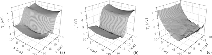
Figure 15. Spatial distribution of the electron temperature in (a) the (x–z)-plane at y = 0, (b) the (y–z)-plane at x = 0 and (c) the (x–y)-plane at z = 10 cm. Reproduced from [65]. © IOP Publishing Ltd. CC BY 3.0.
Download figure:
Standard image High-resolution image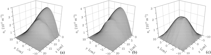
Figure 16. The same as in figure 15 but for the electron density. Reproduced from [65]. © IOP Publishing Ltd. CC BY 3.0.
Download figure:
Standard image High-resolution imageThe explanation of the transport across the magnetic filter and the appearance of these structures involves several drift motions (figure 17). Firstly, the presence of a magnetic barrier reduces the electron transport coefficients (equation (33)). This causes a gradient in the density and a related ambipolar electric field. This drives a drift 7 that shifts the plasma parallel to the extent of the magnetic filter (in vertical direction in figure 17). This effect is complemented by a ∇B-drift that transports the electrons in the same direction. Then in a plasma bounded by walls this transport causes density gradients in this direction that in a combination with the magnetic field of the filter drive a diamagnetic/E × B drift across the magnetic filter (horizontal direction in figure 17). Similar mechanisms are causing also the inhomogeneity in the electron temperature. Note that these effects are not captured by one-dimensional models.

Figure 17. Particle (a) and fluid (b) view on the electron transport across the magnetic filter. The shaded region on the left of the domain is the particle injection area and the shaded region in the middle is the magnetic filter. Reproduced from [66]. © IOP Publishing Ltd. All rights reserved.
Download figure:
Standard image High-resolution imageThe effects covered in this chapter are examples of the interaction of the magnetic field with the plasma, but generally the magnetic field does not interact directly with the RF field sustaining the plasma. Therefore, they can be observed also in other discharge types, e.g. DC or microwave plasma sources. The effects of the magnetic field, specific for RF discharges are covered in the following sections.
4. Electromagnetic wave propagation along a static magnetic field
One of the distinct characteristics of magnetized plasmas is the richness of waves that exist [2, 72, 73]. This is related to the anisotropy of the plasma, introduced by the magnetic field and described by the tensor nature of the plasma conductivity (53) and the dielectric constant (54). While in the isotropic, non-magnetized plasmas the waves with frequencies in the RF region generally cannot propagate, in magnetized plasmas various wave modes in this frequency range can be excited. As we will see in the following sections, this allows maintaining dense plasmas, owing to the fact that the RF energy can be delivered directly into the volume of the discharge since the electric field of the wave is now not confined only to the boundary skin layer like in the case of non-magnetized discharges and the discharges discussed in section 3. Here we will limit ourselves only to those types of waves that are relevant for the discharge maintenance or are commonly used as a diagnostic tool. A more complete spectrum of the wave modes in magnetized plasmas can be found in the respective textbooks, e.g. [2, 72–74].
4.1. General aspects
The characteristics of the electromagnetic waves follow from the dispersion relation that connects the angular frequency ω of the wave with its wave vector  . This relation is obtained from the wave equation

that follows from Maxwell's equations. The dots signify the temporal derivatives and μ0 and ɛ0 are the permeability and permittivity of vacuum, respectively, with c−2 = ɛ0 μ0 the velocity of light. Further, the derivation of this equation considers that in plasmas only free charge carriers are present, i.e. polarisation effects are neglected.
We will concentrate our attention on TE (electro-magnetic) waves. For such waves  and consequently the space charge
  is zero. A Fourier transform both in the space
  and the time domain (∂/∂t → iω) converts the differential equation into an algebraic one
8
:
and the time domain (∂/∂t → iω) converts the differential equation into an algebraic one
8
:

This is a system of homogeneous linear equations for the field components Ex , Ey and Ez . A non-trivial solution exists when:

This expression defines the dispersion relation  or
or  . For completeness we provide also the general form of the dispersion relation for waves that have also a longitudinal component of the electric field, i.e. the wave propagation involves also space charge oscillations ρ ≠ 0:

However, further on we will not be investigating the waves described by this relation (e.g. the x-wave [2]).
When the waves are damped, the frequency or the wavevector become complex:  or
or  . The choice which of the two paths to follow depends on whether we are dealing with an initial value problem (complex frequency) or a boundary value problem (complex wavevector). The damping in time is given by
  and the spatial reduction in the wave amplitude is described as
  . The damping length δ is related to the imaginary part of the wavevector:
  , while its real part is related to the wavelength of the wave: λ = 2π/kr
. In the presence of damping, the dispersion relation is also complex. When the damping is weak, the corresponding imaginary parts can be obtained from the approximate relations [74]:
, while its real part is related to the wavelength of the wave: λ = 2π/kr
. In the presence of damping, the dispersion relation is also complex. When the damping is weak, the corresponding imaginary parts can be obtained from the approximate relations [74]:


where the real part of the frequency, respectively of the wavevector, are obtained from the real roots of  .
.
The frequency at which kr = 0, i.e. λ → ∞, is called a cutoff. When the wave reaches a region in the plasma where the dispersion relation exhibits a cutoff point, the wave is reflected from that region. Beyond the point of the cutoff, the wave exists as an evanescent wave. This is the situation for the classical inductive discharges [3], where the antenna launches an electromagnetic wave with a frequency below the cutoff frequency. The discharge is then sustained by the evanescent wave. If for a finite frequency kr → ∞ (λ = 0), then the wave has a resonance there. At the point of the resonance the wave becomes evanescent and its energy is absorbed by the plasma. This is an efficient way to couple energy into the plasma and is used in the ECR sources, covered further on.
4.2. Waves in unbounded plasmas
The dispersion relation (61) describes three different modes (eigenmodes). The first one has an electric field along the magnetic field lines:  . For this mode holds:

This dispersion relation coincides with the one for the electromagnetic waves in non-magnetized plasmas (including damping due to electron collisions):

Here these waves propagate perpendicularly to the magnetic field  . Since the electric field is parallel to the magnetic field, the electrons can follow the wave oscillations in much the same wave as in non-magnetized discharges. This explains the lack of influence of the magnetic field on this mode. The property can then be used for diagnostic purposes e.g. for microwave interferometry. If the microwave beam is sent across the magnetized discharge in such a way that the electric field oscillates parallel to the B-field, then the phase shift of the wave will not be affected by the magnetic field and the same relations for obtaining the plasma density can be used. Then the phase shift of the wave through the plasma (wavevector kp) relative to the vacuum case (wavevector k0) is

The first relation considers the inhomogeneity in the plasma density that through the plasma frequency influences the wavelength and the accrued phase shift in the plasma. When the plasma length L is known, the line-averaged electron density  can be obtained.
The other two modes propagate along the magnetic field lines and are generally coupled due to the off-diagonal elements ɛ× of the dielectric tensor (54). The reason is that an electric field in the x-direction leads to a displacement of the electrons, i.e. a current along the y-axis due to the E × B-drift. This displacement then creates an electric field in the same direction, that in turn leads to electron displacements along the x-axis. The two modes can be decoupled if circularly polarized fields are considered:

The electric field of the R-wave (minus sign)
9
rotates in the same direction as the electrons, i.e. clockwise following the rule of the right-hand, while the field of the L-wave (plus sign) rotates in the direction of the ion gyration, i.e. counterclockwise and follows the rule of the left-hand (figure 2). Note that the notation R- and L-wave is then related to the direction of rotation with respect to the orientation of the magnetic field and not with respect to the direction of the wave propagation, i.e. the direction of  . Since the latter determines the polarisation of the wave, both waves can be either left or right circularly polarized (figure 18).

Figure 18. Illustration demonstrating the difference in polarization relative to the magnetic field and relative to the direction of propagation. A right circularly polarized wave propagating along the magnetic field lines (right) is an R-wave that can experience an ECR (same direction of rotation as the electron gyration). The same wave propagating against the magnetic field lines (left) is an L-wave that cannot resonate with the electrons.
Download figure:
Standard image High-resolution imageThe dispersion relation of these modes is (top sign for the R-wave, bottom for the L-wave):

For the R-wave a cutoff occurs at the frequencies 0 and ωR while the L-wave has a cutoff at ωL, where

The R-wave has also a resonance at the electron cyclotron frequency. At the resonance the electric field of the wave rotates with the same frequency and in the same direction as the electron gyration. Then, in the reference frame of the electrons, they experience a constant electric field that continuously accelerates them, leading to the resonant absorption of the wave energy. This aspect is the foundation of the ECR sources covered in section 6.
The dispersion relations for the R- and L-waves, together with the characteristic frequencies are illustrated in figure 19. The R-wave exists for frequencies in the range 0 to ωc and ωR to ∞. In the region between ωc and ωR the wave cannot propagate. This is called bandgap. The L-wave can propagate for frequencies that exceed ωL. If the ion motion is also taken into account, the L-wave can propagate also for frequencies between 0 and ωc,i. It then has a resonance at ωc,i and a bandgap between ωc,i and ωL.
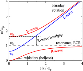
Figure 19. Dispersion relation for the R- and L-waves for the case ωc = ωp. The cutoff and resonance frequencies are also indicated. The region of RF frequencies is usually below ωL.
Download figure:
Standard image High-resolution imageFor very large frequencies (ω ≫ ωp, ωc) the dispersion relations of the two waves approach the dispersion relation for electromagnetic waves in vacuum: k2 = ω2/c2. Nevertheless, small differences in their wavevectors exist, leading to the Faraday rotation. The effect works in the following way. The electric field of a wave with a linear polarisation in a perpendicular direction to the magnetic field can be represented as a sum of an R- and an L-wave (figure 20). After traversing a magnetized plasma of a length L, the phase of the L-wave would be slightly higher than that of the R-wave. The field of the L-wave will then be rotated by an angle α, where

The two waves can again be summed together to a linear polarisation. Due to the phase difference of the L- and the R-wave, the polarisation is now rotated to an angle θ = α/2 relative to the original polarisation. By measuring the angle of rotation the plasma density can be determined when the magnetic field strength is known. This finds applications mainly in the investigations of fusion plasmas [75]. Alternatively, the magnetic field can be inferred if the plasma density is known from other measurements. This approach is commonly used in the astronomy to measure the interstellar magnetic fields [76].
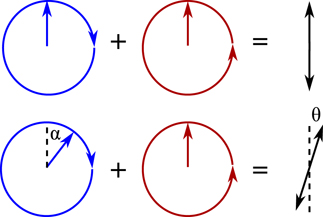
Figure 20. Illustration to the principle of the Faraday rotation. The linearly polarized wave can be represented as a sum of an L- and an R-wave. After traversing the plasma, due to the slight difference in their dispersion relations, the two waves have completed different number of cycles. The resulting linearly polarized wave appears to have rotated its direction of polarisation.
Download figure:
Standard image High-resolution imageThe low-frequency limit of the R-wave is called a whistler wave. For this wave ω ≪ ωc, ωp and

Such waves are excited by lightning strikes and they propagate in the ionosphere along the field lines of the Earth's magnetic field. They can be received by radio-stations at the end of the field line. Since the phase velocity of the wave vph = ω/k increases with the wave frequency the high-frequency components are received first followed by components with decreasing frequencies. The result is a specific hiss which promoted the term whistler [2].
4.3. Bounded plasmas
The dispersion relation (69) is derived for infinite plasmas, i.e. without boundaries. Then the wavevector kR,L has only a component k|| parallel to the magnetic field. In finite-size plasmas the field components are additionally subject to boundary conditions at the surrounding surfaces. For conducting (metallic) surfaces the tangential components of the electric field have to vanish and on non-conducting surfaces the tangential components of the magnetic field have to be continuous across the boundary. The latter condition is equivalent to continuity of the normal derivatives of the electric field. To satisfy these boundary conditions, the electric field of the wave has to have a spatial profile in a direction perpendicular to the direction of propagation, in this case also the direction of the external magnetic field:

This corresponds to the existence in (69) not only of a longitudinal component k|| of the wavevector but also of a TE one k⊥. This TE component is generally fixed by the dimensions of the plasma chamber. The relation is obtained by inserting the ansatz (73) for the electric field into the wave equation (59) and solving for the spatial structure of the field by invoking also the boundary conditions.
We will demonstrate this aspect for the helicon waves. These waves are whistler waves (low-frequency R-wave) modified due to the presence of boundaries. The helicon discharges are sources of very dense plasmas. Their physics and practical aspects are covered in the following section 5.
The relation determining the spatial variation of the amplitude E0 in equation (73) is

where for the helicon waves ω ≪ ωc, ωp holds and  . Note that the latter approximation essentially means neglecting the component ɛ⊥ relative to ɛ×. The physical interpretation is that the electron current induced by the electric field of the wave is not due to cross-field conductivity but due to the E × B-drift perpendicularly to the field:

Note that in this work we explicitly neglect the contribution of the ions. When the ion gyro-motion is also included, additionally the condition ω > ωc,i has to hold. However, even in hydrogen plasmas operated at the standard RF frequency of ω/2π = 13.56 MHz this condition is well fulfilled for magnetic field strengths of up to 0.89 T justifying the omission of the ion motion from the treatment.
The typical situation is cylindrically-symmetric, i.e. E0(x, y) = E0(r)eimφ , with m an integer number defining the azimuthal mode and r the radial coordinate. The solutions in this case are given in terms of the Bessel functions of first kind Jm (x) as demonstrated by Chen [77]. In that work, the structure and the various modes of cylindrically-symmetric helicon waves are derived and presented in a very intuitive way. Here we will not reproduce the rather lengthy results. We will only provide the link between the approach followed here and the path taken by Chen by pointing out that the parameter α defined in [77] is related to the components of the dielectric tensor by [78]:

The dispersion relation of the helicon waves is

The radius R of the plasma vessel determines the transversal wavenumber k⊥ through the boundary conditions [77]:

The prime denotes the derivative of the Bessel function Jm
with respect to its argument. These two equations provide the relation between the wavevector  and the frequency of the wave ω, the magnetic field (through ωc) and the plasma density (through ωp). In the general case (arbitrary m), this relation cannot be obtained explicitly and only approximate numerical solutions are possible. An exact solution is possible only for the azimuthally-symmetric case (m = 0) where k⊥ = λ1,1/R with λ1,1 ≈ 3.832 the first zero of the Bessel function J1(x). In this case the dispersion relation of these helicon waves

differs from the one for the whistler waves (equation (72)) only by a factor  that depends on the wavelength of the helicon wave λ. This illustrates the similarities in the behaviour of the two waves. However, the differences due to the presence of boundaries provide some unique properties of the helicon waves that are important for their practical usage.
5. Helicon plasma sources
In this section we cover the various aspects and details of the application of helicon waves for sustaining a discharge. These waves exist only in the presence of an external magnetic field and do not have an unmagnetized counterpart. The discharges using these waves for plasma production are called helicon discharges and are characterized by very dense plasmas with high degree of ionisation that can easily be operated at very low pressures (at and below 1 Pa). The helicon discharges generally require a specific antenna design and due to the low operational pressures exhibit collisionless heating mechanisms such as Landau damping. This discharge type falls in the category of wave-sustained discharges and shows in general a number of fascinating physical phenomena, e.g. double layer formation. However, due to the strong radial gradients in the plasma density (inhomogeneity) and the complexity of the equipment and discharge design that are required for sustaining them, these discharges find only limited application in specific fields. These various aspects are covered in the following.
5.1. Basic design
The term 'helicon' was first introduced by Aigrain for electromagnetic waves propagating in the free electron plasma within a solid metal [79]. The name comes from the helical trajectory the electric field follows as the wave propagates [80]. Shortly after, the propagation of equivalent waves was studied also in gaseous plasmas. However, they were studied purely as a wave phenomena in the plasma and not as a source of energy for sustaining the plasma. The first proposal to use them to couple energy to the electrons and to sustain a discharge was made in 1970 by Boswell [81, 82]. This has been followed by extensive investigations of the properties and the characteristics of these discharges. The period is covered in a two-part review by Boswell and Chen [83, 84] and in a book chapter by Chen [85]. A review by Chen [80] covers also the more recent developments and trends in the field while Boswell has established a workshop on the physics and applications of helicon plasmas [82]. Shinohara, also among the prominent contributors to the field, demonstrates the main aspects of these sources and shows images from the operation of various helicon sources in a recent review [86].
The helicon discharges have been originally ignited in cylindrical tubes (figure 21 (top)) with an axial magnetic field [83]. The trend continues to this day. These configurations have typically a radius of a few cm and a length of few tens of cm up to over a meter. A series of coils along the length of the tube provide a nearly homogeneous axial magnetic field for the propagation of the helicon waves. Sometimes the magnetic field structure is modified on one or both sides of the tube to realize a magnetic mirror for better plasma confinement and an additional increase of the plasma density.

Figure 21. Schematic representation of typical discharge configurations for sustaining helicon discharges. (Top) Standard cylindrical configuration for study of the discharge properties. Axial plasma confinement through cusp magnetic field can be achieved by switching off the end coils. Reproduced from [80]. © IOP Publishing Ltd. All rights reserved. (Bottom) Modified configuration envisioned for application in semiconductor industry. Such configuration is also used for studies of double layer formation. Reproduced from [87]. © IOP Publishing Ltd. All rights reserved.
Download figure:
Standard image High-resolution imageMotivated by a strive to introduce the helicon discharges into the microelectronics industry, also configurations have been investigated where the helicon tube opens up in a second chamber with a much larger radius (figure 21 (bottom)). This is where the processed wafers could be introduced. To provide an even spread over the wafer of the narrow plasma column from the first tube, the magnetic field in the second chamber is let to diverge. Despite their promising characteristics, the helicon discharges have not been adopted on a large scale for industrial applications [80]. Nevertheless, the investigations of this two-chamber configuration revealed some interesting phenomena, such as double layer formation (see below).
5.2. Antenna design and mode structure
The antennas for the helicon discharges are tailored to induce a field structure similar to the one of the wave. The structure of the electric field of the wave is obtained as a solution to equation (74). In cylindrical coordinates the solution is characterized by the azimuthal mode number m and its radial distribution is given by Bessel functions [77]. The field distribution for the most common cases m = 0 and m = +1 are illustrated in figure 22. At each point in the transversal cross section the direction of the electric field rotates as the wave propagates forwards, in accordance with the ansatz for ER in equation (73). The electric field drives an electron current with density described by equation (75) which also twists along the direction of wave propagation (figure 23). The field of the other base configuration, the m = −1 mode, bears some similarity to the one of the m = +1 mode (figure 24). However, this mode is more difficult to excite and is less efficient in sustaining a discharge (a longer plasma column is sustained by the m = +1 mode [88]).
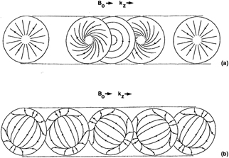
Figure 22. Structure of the field lines of the TE electric field of a helicon wave with (a) m = 0 and (b) m = +1. The orientation of the external magnetic field and of the longitudinal wavevector k|| ≡ kz are also shown. Reprinted from [89], Copyright (1994), with permission from Elsevier.
Download figure:
Standard image High-resolution image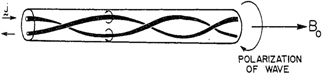
Figure 23. Sketch of the current density in the plasma column for the m = +1 mode. Reproduced from [90]. © IOP Publishing Ltd. All rights reserved.
Download figure:
Standard image High-resolution image
Figure 24. Electric (dotted) and magnetic (solid) field lines of the m = +1 (left) and the m = −1 (right) azimuthal modes for a uniform plasma. Reproduced from [80]. © IOP Publishing Ltd. All rights reserved.
Download figure:
Standard image High-resolution imageThe m = 0 azimuthal mode can be launched by the standard antennas used for inductive discharges [3, 91]. Both the flat spiral antennas and the cylindrical solenoid type coils induce a circular (azimuthal) electric field configuration that easily couples to the same field configuration depicted in the middle cross section in figure 22(a). To excite the m = +1 or the m = −1 mode, the field configuration depicted in figure 24 has to be induced. This requires a special antenna design. Several different configurations have been developed to this end, the most widespread ones are shown in figure 25. A common trait is that they have probably one of the most complex design among all discharge antennas. The higher helicon modes (|m| > 1) have an even more complex field structure that makes it rather challenging to design an antenna that couples exclusively to one of these modes.

Figure 25. Half-wavelength antenna configurations for m = 1 helicon discharges: (A) Nagoya type III, (B) Boswell type, and (C) Shoji (helical) type. The arrows indicate the current flow at a given instant. Reproduced from [92]. © IOP Publishing Ltd. All rights reserved.
Download figure:
Standard image High-resolution imageThe underlying idea of the antenna designs in figure 25 is to create the twisted structure of the electric field (figure 22(b)). The amount of the twist is fixed by the length L of the antenna which then determines the wavelength λs
= 2L/(2s + 1) and the longitudinal wavenumber k|| = 2π/λs
. The integer number s gives the longitudinal mode. From here follows a peculiarity of the helicon discharges: the plasma density is actually determined by the dispersion relation (77) and not by the balance of the electron energy as is usually the case in most discharge types. The longitudinal and the transversal parts of the wavevector are fixed by the antenna size and by the discharge tube dimensions (via the boundary condition (78)), respectively. Then  is also fixed and for a given RF frequency ω and a set magnetic field B0 the plasma density n is uniquely defined. As a consequence the electron density remains nearly constant until a jump in another longitudinal mode becomes energetically more favourable.
The linear scaling of the electron density with the magnetic field (figure 26) has been established already in the pioneering works on helicons [90]. Superimposed on that are the aforementioned mode jumps. The helicon discharges often exhibit also longitudinal mode jumps due to the formation of standing waves in the source (cavity modes) due to the reflection of the helicon wave at the end plates. These have been observed both with antennas exciting the m = +1 azimuthal mode, e.g. in reference [87], as well as in discharges with planar coils operating in the m = 0 mode, e.g. in [91] (figure 27). For the m = +1 mode the density jumps due to these cavity modes are usually more pronounced than the jumps due to the size of the antenna.
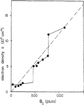
Figure 26. Variation of the radially averaged plasma density with the strength of the magnetic field. The continuous curve is a fit to the experimental data and the dashed curve is the prediction from the dispersion relation for whistler waves. Reproduced from [90]. © IOP Publishing Ltd. All rights reserved.
Download figure:
Standard image High-resolution imageThe behaviour of the plasma density with the power in helicon discharges is well illustrated by figure 28. As discussed, the plasma density no longer scales with the RF power, but remains nearly constant until the next mode becomes energetically more favourable. In this case, the density jumps are related to changes in the wavelength of the helicon wave, i.e. changes in k||. This is demonstrated in figure 29 through measurements of the wave field for the different density regions. The nodes of the standing wave pattern seen both in the amplitude of the field as minima and in its phase as phase jumps are a measure for the wavelength, i.e. for k||. The change of the wavelength is then visible by the change in the distance between the nodes. At higher power levels the distance and correspondingly the wavelength are shorter, i.e. k|| is larger. Then also α in equation (77) increases due to a higher density permitted by the energy balance of the electrons.
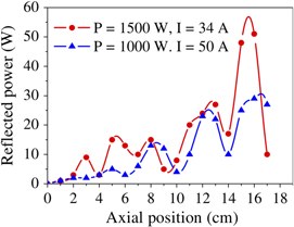
Figure 27. Standing wave patterns of the reflected power as a function of the discharge length at a neutral gas pressure of 0.5 Pa and two different discharge conditions. The legend provides the values of the RF power and the current through the coil creating the static magnetic field. The curves are splines to guide the eye. Reproduced from [91]. © IOP Publishing Ltd. All rights reserved.
Download figure:
Standard image High-resolution image
Figure 28. Variation of the ion saturation current to a Langmuir probe, i.e. of the plasma density with the RF power for a fixed value of the magnetic field. Reproduced from [87]. © IOP Publishing Ltd. All rights reserved.
Download figure:
Standard image High-resolution imageThe helicon discharges in the azimuthal m = 0 mode are created by a standard antenna for an inductive discharge. These antennas do not set the longitudinal wavevector. However, standing waves corresponding to the cavity modes of the discharge chamber still appear (figure 27). The standing wave patterns in the reflected power observed in [91] can be understood as follows. For a given value of the RF power and the magnetic field, the reflected power is minimal when the chamber length is sufficient to fit a whole number of half-wavelengths, as determined by the dispersion relation (77). This happens for a specific value of the plasma density which requires a given amount of power to be absorbed by the plasma, in accordance with the electron energy balance equation. Any additional power is not absorbed and is returned as reflected power.

Figure 29. Axial variation of the longitudinal magnetic field of the wave for the W1, W2 and W3 modes in figure 28: amplitude (top) and phase (bottom). The measurements cover the entire length of the discharge but are performed with two different probes, inserted from the two ends of the chamber. The left and right panes show the results from each of the probes. The measurements are taken in the source in figure 21 (bottom) where also the position of the helicon antenna is marked. Reproduced from [87]. © IOP Publishing Ltd. All rights reserved.
Download figure:
Standard image High-resolution image5.3. Electron heating mechanisms
The helicon plasmas belong to the special class of wave-heated discharges. They rely on the interaction of the plasma with the wave: as the wave propagates, it transfers its energy to sustain the plasma while the plasma provides the conditions for the propagation of the wave in accordance with the dispersion relation [30]. The wave propagation was covered in the previous subsection and here we will briefly discuss the mechanisms behind the energy dissipation of the helicon waves.
The dissipation of the wave energy and the plasma heating are described by a term of the form  . However, when the current density is given by the relation (75), the scalar product in Q is zero, i.e. in the idealized treatment the dissipation was neglected and the helicon wave could not sustain a discharge. For a transfer of energy, the electric field needs to have a finite component along the direction of the current density, i.e. in a direction parallel to the static magnetic field B0. In this case Chen [77] has shown that the wave decomposes into two branches. One of them corresponds to a dissipative helicon mode. The other mode is the electrostatic Trivelpiece–Gould mode [94]. This latter mode is highly damped due to the strong dissipation of its energy. Unlike the helicon mode, whose fields peak on the discharge axis, the field of the Trivelpiece–Gould mode (figure 30) is concentrated close to the radial boundaries of the plasma.
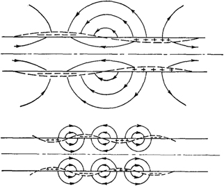
Figure 30. Schematic representation of the electric field configuration and the space charge for the azimuthally symmetric surface wave of the Trivelpiece–Gould mode. The cylindrical plasma column is in the middle surrounded outside by vacuum. Reprinted from [94], with the permission of AIP Publishing.
Download figure:
Standard image High-resolution imageIt has been proposed that the efficient plasma production in the helicon discharges is due to coupling of the helicon wave to this highly dissipative mode [95], i.e. the helicon wave excites a Trivelpiece–Gould mode which then efficiently transfers its energy to the plasma electrons that sustain the ionization. The existence of the Trivelpiece–Gould mode together with indications for its contribution to the plasma heating have been provided in [95, 96]. However, this hypothesis has been strongly contested [85] in favour of other mechanisms. The alternatives that have been considered include the usual electron-neutral collisions related to the standard ohmic (collisional) heating, Coulomb collisions as well as linear and non-linear wave–particle interactions (Landau damping). The collisionless Landau damping is often the leading candidate. Its rate νLD is usually estimated by using the classical formula [77]:

where ζ = ω/kvth with  the thermal velocity of the electrons. For example in references [91, 97] the authors have obtained very good agreement between the measured axial structure of the helicon wave and an analytical model, which includes a damping rate whose value is in good agreement with the one predicted by equation (80). It is possible that the heating mechanism will remain a matter of debate as the leading mechanism for energy absorption depends on the particular discharge, e.g. through the antenna design or chamber geometry, and experimental conditions so that the different experiments can provide contradicting conclusions.
At low power levels the helicon discharges exhibit also operation in the E- and H-mode (figure 28). These mode transitions are related to changes in the power coupling mechanism. Similarly to the inductive discharges [3], the helicon discharges initially ignite in a capacitive E-mode, i.e. the discharge is sustained by the oscillating electric field that exists due to the voltage drop over the helicon antenna. At a given power level, the discharge transitions into an inductive H-mode. In this mode the current in the antenna creates oscillating magnetic field that induces the electric field sustaining the discharge. The plasma density in these two modes have the classical behaviour with the power, characteristic for capacitive and inductive discharges [3].
Both in the E- and in the H-mode the power is not sufficient to maintain the plasma density necessary for the propagation of the helicon wave. Only at higher power the plasma density allows the dispersion relation of the helicon wave (equation (77)) to be satisfied. A helicon wave is launched and the discharge enters the W-mode (W for 'wave'). The energy of the helicon wave is efficiently coupled to the plasma electrons, producing another jump in the density (figure 28). As discussed, further increase of the power leads to other jumps in the density, related to various modes of the helicon wave.
Lieberman and Boswell [98] have described the mechanism of the E-H-W mode transition in the frame of a global model. However, the model does not include the collisionless power absorption (Landau damping). Since it also considers only a simplified geometry of the plasma, the results of the model provide only the qualitative picture of the processes. The situation is similar to the E-H mode transition in non-magnetized discharges. The energy losses of the electrons scale linearly with their density, while the power coupling efficiency through the different channels (capacitive, inductive and wave heating) depend in a non-linear manner on it (figure 31). The crossing point between the curves for the power input and the power losses determine the electron density, i.e. consistent with their energy balance. As the power to the antenna is changed, the crossing point shifts and provides the new density. The wave heating channel has generally a multitude of maxima (figure 32(a)), corresponding to the resonant conditions when the wavelength of the helicon wave matches the conditions for the cavity modes. As with their non-magnetized counterparts, at low plasma densities the capacitive power input channel dominates also in the helicon discharges (figure 32(b)). However, as the density increases, the W-mode quickly becomes the dominant one. The range where the H-mode is the leading heating mechanism can vary, depending on the magnetic field strength, antenna design and other parameters [79].
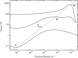
Figure 31. Schematic representation of the power balance for the E-H-W transitions in a helicon discharge. Reproduced with permission from [79]. © Cambridge University Press.
Download figure:
Standard image High-resolution image
Figure 32. (a) Contributions of the different power coupling channels to the electron energy balance as a function of the edge electron density at an antenna voltage of 300 V, a pressure of 3 mTorr and a vessel length of 50 cm. Electron losses (straight line), capacitive (decreasing dashed line), inductive (dotted curve) and wave (increasing dashed line) power input channels together with the net power input (curve with dots). (b) Relative contribution of the different power input channels—capacitive (continuous curve), inductive (dashed curve) and wave heating (curve with dots). Reproduced with permission from [98].
Download figure:
Standard image High-resolution image5.4. Applications
From the physics perspective there is no doubt that the helicon discharges are an interesting subject to explore. However, the elaborate and costly equipment needed for their ignition together with the limited flexibility in the plasma parameters due to the resonant nature of the excitation of the helicon waves has vastly limited their field of application. Furthermore, the helicon discharges create dense plasmas only in a narrow region near the axis, as evidenced also by the plasma emission [97]. Examples for their use in the semiconductor industry for deposition and etching do exist [99–102], but the helicon plasmas are far from the dominating type of discharges there. However, the helicon discharges seem to enjoy a renaissance period in the recent years due to their ability to produce plasmas with high degree of ionization at low pressures [77]. This is also due to the emergence of novel fields of plasma applications, where such types of plasmas are highly beneficial. Prominent examples are the ion and plasma thrusters and the production of energetic beams of particles for use in fusion and particle accelerators.
A development area in the recent years for the application of helicon discharges are the plasma thrusters [103–105]. A prominent example is the variable specific impulse magnetoplasma rocket (VASIMR) [104] where the propellant is ionized using a helicon discharge. VASIMR can operate with different propellants, but hydrogen and argon are the preferred ones due to price considerations and other factors. Another commonly used propellant gas is xenon due to the large mass and hence impulse of the ions together with its low ionization energy. The high efficiency of the helicon plasma creates an ionization degree close to 100%. The ions are then heated by an ion cyclotron resonance heating, ICRH (figure 33), which is analogous to the electron cyclotron heating discussed in the next section. Afterwards, the ions are accelerated through a magnetic nozzle to create a thrust. Such devices show very promising results [106] motivating an ongoing active development in search for an optimized and flexible configuration.

Figure 33. Schematic layout of the VASIMR plasma thruster. Reprinted from [107], with the permission of AIP Publishing.
Download figure:
Standard image High-resolution imageThe period of active development of electric propulsion systems, i.e. ion and plasma thrusters, roughly coincides with the period of discovery and intensive investigations on current-free double layers in helicon discharges [108]. It is then unsurprising that thrusters based on discharges with double layers have been also proposed [109]. A double layer is a thin (typically few tens of Debye lengths) region in the plasma volume where the quasi-neutrality is violated. Its appearance is associated with the transition between the narrow discharge tube and the large expansion chamber (figure 21 (bottom)) where also the magnetic field lines strongly diverge [108, 110]. At the position of the double layer the plasma parameters and most notably the plasma potential exhibit a jump (figure 34). The electric field associated with this jump in the potential accelerates the plasma ions, leading to the formation of beam of energetic particles [103] which can create a thrust.

Figure 34. (a) Plasma potential and (b) plasma density measured with an energy analyzer along the z-axis in a plasma chamber with the configuration in figure 21 (bottom) at an argon pressure of 0.2 mTorr and 250 W RF power. Reprinted from [108], with the permission of AIP Publishing.
Download figure:
Standard image High-resolution imageCombined with the high ionisation efficiency, the helicon discharges are attractive sources for electrical propulsion applications. The high degree of ionisation makes them also good candidates for the production of negative hydrogen ions for use in the current drive and heating systems in fusion applications [111, 112]. Currently, the most efficient way for producing negative hydrogen and deuterium ions is by electron capture on caesiated surfaces with low work function. The process is most probable when atomic ions or neutrals collide with the surface. For the production of large amount of negative ions, high dissociation and ionisation degrees are favourable. Such conditions are expected in helicon discharges which motivates the interest in them [111, 112].
Another direction of investigations for the application of helicon plasmas is as wake-field accelerators [113]. The idea is to create a distortion in the quasi-neutrality in a dense plasma. The perturbation is created by a resonance between the beat frequency of two laser beams and the plasma frequency. The electric fields in the perturbed region can easily reach strengths in the range of MV m−1. The space-charge region is pushed along the plasma column by the laser beams. A beam of charged particles moving synchronously with the perturbation could then be accelerated to relativistic energies with a table-top device. The source would be separated into several sections (figure 35) with different densities to compensate for the change in the plasma frequency due to the relativistic effects. The challenge here is to create a plasma column with a density of the order of 1017 cm−3 over a distance of a few meters with a uniformity better than 1%. Large plenum would provide a reservoir of neutral gas to be sucked into the plasma column and ionized during the plasma pulses. However, various difficulties make the realization of this concept a challenging task [114]. Possibilities to reach TeV energies in a single stage by using proton bunches instead of lasers to produce the wake field are also considered [115].

Figure 35. Conceptual layout of a single stage of a wake-field accelerator. Reprinted from [113], with the permission of AIP Publishing.
Download figure:
Standard image High-resolution imageThe helicon discharges and their theory are tightly related also to other types of discharges. A prominent example is the neutral loop discharge. In this discharge, the magnetic field configuration forms a neutral loop—a circular region where the magnetic field strength vanishes (figure 36). This is achieved by flowing current in opposite directions through two neighbouring magnetic coils. Adding a third one allows the position of the neutral loop to be controlled. The discharges ignited in this field configuration by a common inductive antenna are known as neutral loop discharges. They are characterized by a bright plasma region with a torus shape just below the antenna. Initially, it was thought that the plasma in the torus is heated through a novel collisionless mechanisms involving the meandering motion of the electrons in the region of the separatrix [116]. However, systematic investigations [91] have revealed that the discharge is actually a special kind of helicon plasma. The inductive antenna launches a helicon wave while also sustaining the plasma in the torus region situated in the cusp region beneath the RF antenna. That region acts as a second inductive antenna with an RF current flowing in the opposite direction as that in the external antenna. The fields of the two antennas are superimposed on each other. The result is a modified helicon wave that is characterized by two transverse wavenumbers, the second one being created by the plasma current. This multimode structure of the helicon wave in the neutral loop discharge provides better stability, i.e. larger insensitivity towards the cavity modes of the plasma chamber [97].

Figure 36. Schematic representation of the magnetic field configuration for the production of neutral loop discharge. Reproduced from [116]. © IOP Publishing Ltd. All rights reserved.
Download figure:
Standard image High-resolution imageWhen the neutral loop is shrunk to a point on the axis of the discharge, a magnetic X-point is formed. The discharge ignited in this magnetic field configuration is called X-point discharge [117, 118]. In the plane of the magnetic null point, the magnetic field has only a radial component and thus acts similarly to the magnetic filter, discussed in section 3.2. The result is separation of the discharge into two regions—a bright region close to the RF antenna and dark region in the volume past the X-point plane [119]. The discharge intensity also depends on the radius of the chamber. When the radial magnetic field lines in the plane of the X-point fall into a flange of the chamber, a more luminous plasma forms in those regions (figure 37). This phenomenon is not yet fully understood and shows that magnetized discharges still offer rich field for investigations.
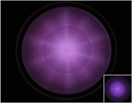
Figure 37. Head-on view of the X-point discharge operated in hydrogen at 0.5 Pa. The inset shows the same discharge with slightly different axial position of the X-point. © [2011] IEEE. Reprinted, with permission, from [117].
Download figure:
Standard image High-resolution image6. ECR plasma sources
In this last section we cover another type of discharge that can exist only in the presence of an external magnetic field. It is based on the resonance absorption of the energy of a circularly polarized electromagnetic wave, when the wave frequency matches the local electron cyclotron frequency. This energy transfer mechanism is also very efficient and allows sustaining dense plasmas with high degree of ionisation. In this section we show the basic design and experimental arrangements for maintaining the discharge and cover some of the fundamental aspects of power absorption as well as discuss some of the applications of such discharges.
6.1. Basic setup
The ECR sources, also known as electron cyclotron resonance ion sources (ECRIS), have been developed in the 60s and 70s of the 20th century [120, 121]. They are widely utilized in the semiconductor industry, as plasma propulsion systems, as sources of highly charged ions for accelerator applications and in many other fields [120, 122, 123]. The operation of these sources relies on the ECR. It occurs for the R-wave when the local cyclotron frequency matches the wave frequency (ωc → ω). In the vicinity of the resonance point, the energy of the wave is fully transferred to the plasma electrons, making this one of the most efficient power coupling mechanisms. The result is dense plasmas with high degree of ionisation. Another characteristic feature of the ECR discharges is that they operate at low pressures (around or below 0.1 Pa) since the collisions interfere with the cyclotron heating. This is what makes them attractive for the semiconductor industry since the low collisionality of the particles allows for preparation of structures with large aspect ratios.
The ECR discharges for commercial applications are usually operated at a frequency ω/2π = 2.45 GHz which corresponds to the electron gyro-frequency at a magnetic field strength of B0 = 87.5 mT [120]. Usually, the R-wave is launched in a region of strong magnetic field (ωc > ω) and the resonance point is reached as the wave propagates along the inhomogeneous (diverging) field (figure 38). The electromagnetic radiation is supplied through a waveguide that ends with a quartz window facing the plasma chamber (figure 39). Technically, these discharges do not belong to the class of the RF discharges. The generation of the much higher frequencies of the microwave radiation requires generators based on different physical principles. Furthermore, at these frequencies the wave nature of the radiation is much more pronounced which necessitates the use of waveguides for the transportation of the energy. Consequently, also a different approach for impedance matching is needed, as evidenced in the figure (stub tuners to match the wave impedance of the waveguide to that of the coupler and a circulator in a combination with a dummy load to isolate the microwave source from the reflected wave). All this additional specialized equipment makes the use of microwaves for sustaining a discharge a costly endeavour. Alternatives, based on waves or resonances in the RF region of the spectrum are therefore much more attractive due to their cost efficiency. An example for such an alternative are the helicon discharges, discussed in the previous section. There, through a clever antenna design and magnetic field configuration, one can also create high-density plasmas. Nevertheless, microwave discharges are included here, since their operation is based on physical principles that are closely related to the topics covered.

Figure 38. Schematic representation of a typical source configuration for ECR discharges (top). The magnetic field lines and the position of the ECR point are also shown. Profile of the magnetic field strength on the axis (bottom). Reproduced with permission from [124].
Download figure:
Standard image High-resolution image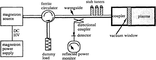
Figure 39. Principle of operation of the system for coupling the electromagnetic radiation in an ECR source. Reprinted from [120], Copyright (1995), with permission from Elsevier.
Download figure:
Standard image High-resolution image6.2. Electron heating mechanism
To illustrate the principle of ECR heating, we consider the motion of an electron in a static, homogeneous magnetic field  under the influence of an electric field that oscillates at the cyclotron frequency ωc. Then the force in the equation of motion (4) that acts on the electron is expressed in a form similar to relation (68):

where E0 is the amplitude. Following the same procedure as in section 2.2, one obtains that the two velocities  and
and  are exactly equal and add up to
  . Note that here these terms are oscillating at ωc
 and their variation cannot be neglected on the time scale of the gyro-motion, as was done in section 2.2. In this case equation (8) takes the form

The solution to this equation is

Note that the magnitude of the transversal velocity of the electron increases linearly with time and the kinetic energy quadratically:

The result also does not depend on the strength of the magnetic field.
Within this model potentially unlimited energies can be reached. However, collisions and electron movement along the magnetic field lines limit the energy an electron gains from the wave. The latter effect is usually the dominant one in practical applications. The mechanism is the following. The electrons are moving in an inhomogeneous magnetic field and the resonance condition is met only in a narrow region. Due to the finite velocity of the particles along the magnetic field, the electrons spend only a finite time in the resonant zone and the energy gain is also finite.
This situation can be described by turning again to the equation of motion (4) of a single electron with an electric force given by (81). This time the strength of the magnetic field varies along the field lines, i.e. along the z-direction  . This field does not fulfill the Maxwell equations but can be used as an approximation for the magnetic field in the vicinity of the resonance point. The equation of motion is solved using the ansatz

where f(t) and g(t) are functions that determine the transversal velocity v⊥. Following the approach in [1, chapter 13.1], vz
is considered to be constant, i.e. the magnetic mirror effect is neglected. Then the magnetic field seen by the electron due to its motion changes in time:  with z(t) = vz
t, assuming that the resonant point ωc = ωc,0 is at z = 0 and the electron passes through it at t = 0. Substituting the quantities in the equation of motion (4) and integrating from a time t = −τ to t one obtains for the transversal velocity
with z(t) = vz
t, assuming that the resonant point ωc = ωc,0 is at z = 0 and the electron passes through it at t = 0. Substituting the quantities in the equation of motion (4) and integrating from a time t = −τ to t one obtains for the transversal velocity

Here the magnetic field has been expanded up to a linear order in the vicinity of the resonance point ωc(z) = ωc,0 and the gradient length L at that point and the characteristic width of the resonance zone Λ are defined as [1, chapter 13.1]:

The phase

is not relevant for the final result. The energy gain of the electron, as a function of the distance z = vz t to the resonance point, is then

The function G(z) is given in terms of the normalized Fresnel integrals [125, equations (7.2.7) and (7.2.8)] C(x) and S(x), which here can also be expressed by a single integral:

and is plotted in figure 40. The oscillations are due to the mismatch between the frequency of the electric field and the local cyclotron frequency outside the resonance point. The limiting value for large z is 2 which makes the result of equation (89) identical to [1, equation (13.1.11)].

Figure 40. The function |G(z)|2 in (89) that describes the variation of the energy Δɛ gained by an electron coming from minus infinity (−τ → −∞) as it passes through the ECR resonant zone at z = 0.
Download figure:
Standard image High-resolution imageThe power coupled to the plasma per unit area perpendicular to the magnetic field is then estimated from the flux nvz of the electrons entering the resonance zone and the energy gained by each electron Δɛ as z → ∞ [1, chapter 13.1]

Interestingly, the final result does not depend on the transit time through the resonance region, only on its size L. This result does not change if also the collisions of the electrons with other particles are considered [1].
The description of the actual situation of wave propagation along an inhomogeneous field near the cyclotron resonance is rather involved. The propagation of an R-wave in a magnetic field which strength varies along the direction of wave propagation, i.e. ωc depends on the coordinate z, is described by (cf equation (69)):

The solution to this equation has been obtained in [126] and is rather complicated. However, it allows the calculation of the wave transmission, absorption and reflection at the resonance point. The absorbed power Pabs as a fraction of the incident power Pi is

where

The fraction of transmitted power is

and there is no reflection. For a typical value of L = 0.1 m and a plasma density of n = 1018 m−3, the parameter η has a value close to 70. This means that the incident wave power is completely absorbed at the resonance point.
At low plasma densities, i.e. low values of ωp and thus η, part of the wave energy can be transmitted beyond the resonance point. It is then possible that the wave tunnels through the bandgap of the R-wave (see figure 19) and propagate downstream. The width of the bandgap is

and decreases with the plasma density, which further enhances the possibility for tunneling.
The physical mechanisms behind the wave absorption at the cyclotron resonance contain a number of other aspects that we will only briefly mention here without going into their details. The first aspect is that due to their motion along the magnetic field lines, the electrons exhibit the cyclotron resonance not exactly at the cyclotron frequency, but at a Doppler-shifted one [1, chapter 13.1]:

However, the effect is usually weak and the resonant magnetic field is shifted by typically only a few percent.
If the magnetic field decreases further, it is possible for the electrons to experience resonant heating also at the second and higher multiples of the cyclotron frequency. Further aspects are related to parametric instabilities and non-linear power absorption. If the energy of the wave is too high, its electric and/or magnetic fields can lead to non-linear interactions with the plasma, like ponderomotive force effects, field ionisation, etc. Note that the treatment here as well as the derivation of the dispersion relation of the waves in section 4 consider only the linear contributions and thus explicitly neglect such non-linear effects.
A final aspect to mention is the possibility for chamber geometry resonances, similarly to the cavity modes observed in helicon discharges. However, due to the index of refraction of the plasma, the wavelength of the microwaves are usually of the order of few cm and are much shorter than the chamber dimensions, while vacuum wavelength is much larger than the chamber size. Consequently, these effects are usually not observed. They could possibly play a role during the discharge ignition, during which phase the plasma density and consecutively also the refraction index are still low [120]. These effects can further be influenced also by the transversal structure of the magnetic field. In the treatment here we considered the external magnetic field B0 to vary only along the direction of its field lines. However, its strength varies also in the transverse direction leading to a gradual change of the plasma index of refraction along the radius of the plasma vessel.
6.3. Applications
The high efficiency of energy coupling to the plasma electrons together with the confinement by the static magnetic field needed for the resonance lead to very dense plasmas with high degrees of ionisation. In fact, the ECR discharges are characterized by an abundance of multiply charged ions of the parent feed gas. This makes these types of sources particularly suitable as sources of highly-charged ions for use in particle accelerators and colliders, hence the name ECRIS.
Since the time of their development, the ECR sources are used also for applications as thrusters. Their ability to create dense plasmas at high vacuum levels is a natural advantage here. The operation of the ECR thrusters relies on the diverging magnetic field, needed for the cyclotron resonance. Due to the diamagnetic nature of the plasma, the electrons are pushed out towards the region of weaker field. To preserve the charge balance, the ions are dragged along with them and accelerated to create the thrust.
ECR sources find also applications in the semiconductor etching industry. Their capability of sustaining dense plasmas at low pressures are attractive e.g. for the etching of high-aspect ratio features in chips and integrated circuits. However, from a plasma processing point of view, the cyclotron sources have also certain disadvantages. On one hand, the static magnetic field that is needed is relatively high and it is costly to sustain such a field strength. On the other hand, the energy distribution is characterized by a rather high degree of anisotropy—the cyclotron heating strongly enhances the movement in the directions perpendicular to the magnetic field lines, while along the magnetic field the electron movement is barely affected. The anisotropy in the distribution function leads to differences in the plasma behaviour along and perpendicular to the magnetic field. Further, the presence of energetic electrons leads to the formation of high-voltage sheaths due to the charging of the semiconductor material being processed. The result is charge-effect damage which is detrimental for 'ultra large scale integrated' circuits. Finally, the efficiency of the cyclotron heating is reduced by the electron collisions since this interrupts the acceleration cycle during the gyro-motion. Therefore, the ECR discharges typically operate at very low pressures (0.1 Pa or lower).
7. Conclusions
This paper is a continuation of the previous one [3] where the fundamentals of non-magnetized RF discharges have been presented. In this second part we touch on the plethora of physical phenomena occurring in RF discharges with an external magnetic field present. The goal is to give a glimpse in the topic that could serve as an entry point for newcomers and provide relevant references for further reading. However, effort was put to make this paper also useful as a quick reference for readers already in the field by providing a summary of the most prominent effects, relations and results.
The presence of the magnetic field forces the charged particles to gyrate around its field lines. When another force acts on these particles a variety of drift motions emerge. Further effects of the magnetic field covered here are the reduction of the particle and the energy transport perpendicular to the field lines. This builds the foundation for the propagation of a variety of electro-magnetic waves through the plasma. The use of some of these waves for diagnostic purposes and for sustaining various types of discharges have been outlined. The focus here has been put on the helicon and the ECR sources. Their principles of operation and their applications have been outlined. Other types of RF discharges have also been presented where the imposed external magnetic field does not directly influence the interaction between the RF field and the discharge. A collection of primary sources, classical works and recent publications is offered as an extension of the material provided here.
Acknowledgments
The authors are grateful to the Editors for the opportunity to prepare this paper and especially to the Associate and Guest editor in charge Luís Alves for his understanding and patience when extending the deadline. TVT acknowledges the financial support by the German science foundation (DFG) within the Project 'Transient atmospheric plasmas: from plasmas to liquids to solids' (SFB 1316).
Data availability statement
No new data were created or analysed in this study.
Footnotes
- 3
'Longitudinal' and 'transversal' here pertain to the orientation of the magnetic field relative to the field lines of the RF electric field.
- 4
Usually the term 'cyclotron frequency' is used to denote the angular frequency ωc. However, some authors use this term to denote the linear frequency fc = ωc/2π. Care has to be taken, which of the two is meant.
- 5
The expressions in this work are derived with the convention that the quantities oscillate in time like exp(iωt). Note that some authors assume a dependence in the form exp(−iωt). The two approaches are fully equivalent, the expressions are simply complex conjugates to each other but this leads to differences in the signs in some of the expressions. This can be confusing and can sometimes lead to serious mistakes. The reader is herewith warned and advised to work with only one of the two conventions and to never mix expressions from different conventions.
- 6
'Longitudinal' and 'transversal' here again pertain to the orientation of the magnetic field relative to the field lines of the RF electric field.
- 7
When the potential and the electron density are interconnected through a Boltzmann relation, the diamagnetic and the E × B drift become identical. In such cases, the drift can be termed as either of the two.
- 8
In this work we have chosen the convention for plane waves in the form
 . This corresponds to a wave propagating in the positive spatial direction, while being consistent with the treatment in section 2.5. Naturally, any other choice of the signs in the exponent is possible and would lead to the same results, but some of the expressions would change sign. The reader has to be aware of this possible downfall when consulting the literature.
 - 9
The sign depends on the choice of sign in the exponent. For a time dependence exp(−iωt) the R-wave would have a plus sign in the vector component and the L-wave would correspond to a minus sign. This is related to the necessary phase shift of the y-field component relative to the x-component.

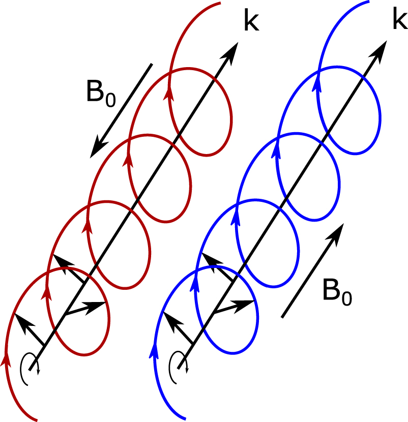
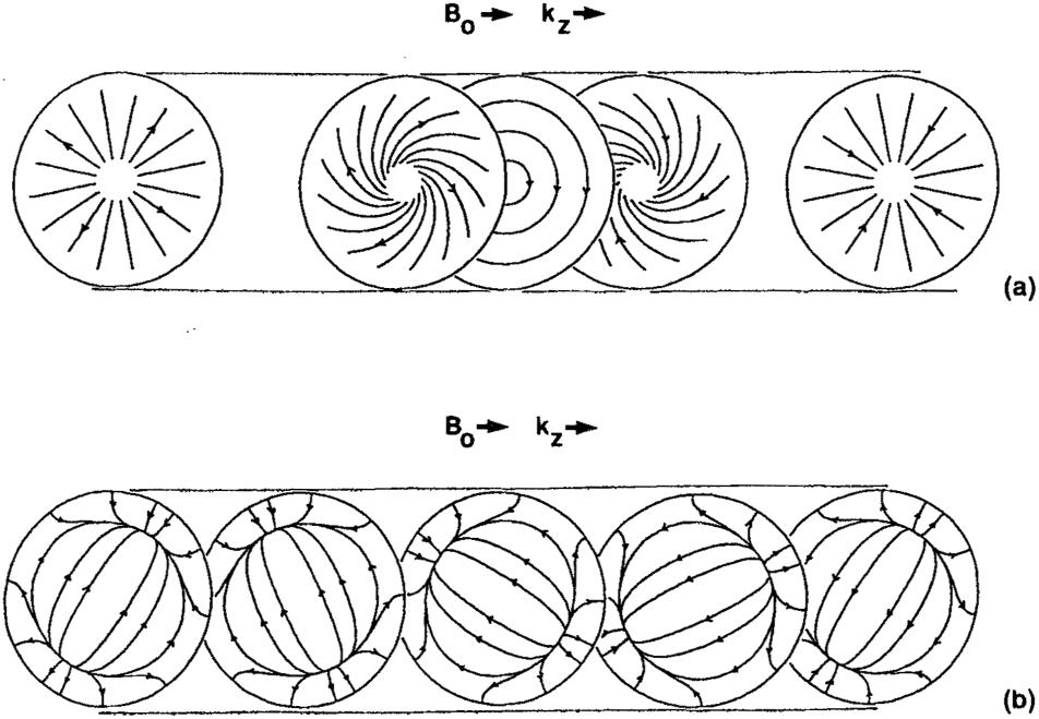
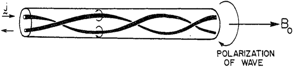
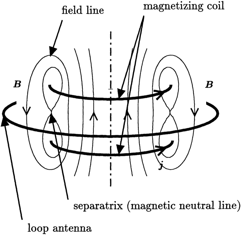
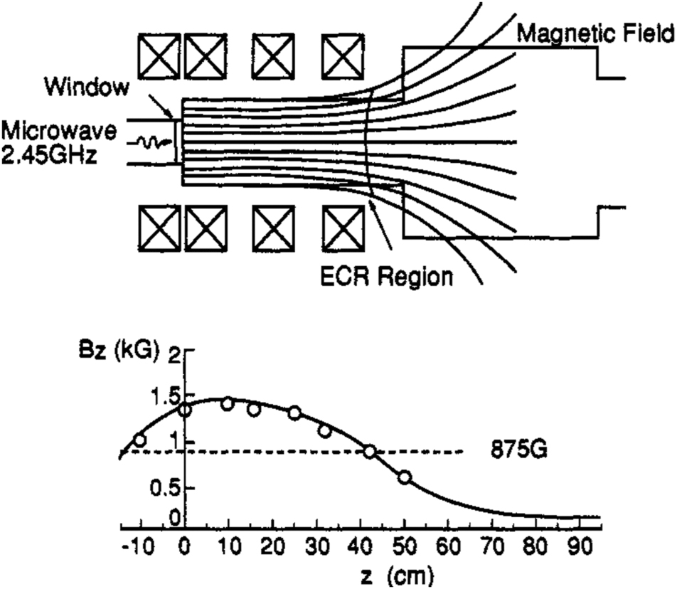