

Abstract
In this study, gas-density variations occurring in pulsed streamer discharge at atmospheric pressure were quantitatively measured using a Mach–Zehnder interferometer. Experiments were performed using different gas compositions involving N2 or air in humid or dry conditions. Spatiotemporal variations in the gas density after the discharge were characterised in terms of the energy relaxation process of the molecules. The measured gas-density variations were well reproduced by a zero-dimensional simulation model of vibrational-to-translational energy transfer in humid-air and humid-N2 conditions. This indicated that the vibrational energy relaxation of N2 through water molecules has a major effect on the gas density. However, the gas-density variations in dry-air and dry-N2 conditions were not reproduced by the model; the corresponding etiology is outlined and discussed.
Export citation and abstract BibTeX RIS
1. Introduction
Atmospheric-pressure plasma can easily produce chemically active species in gas because of the generation of high-energy electrons through discharge, which can induce various chemical reactions [1]. Because atmospheric-pressure plasma does not require a vacuum system, the equipment cost can be reduced, and vacuuming-less processing can become possible. Hence, atmospheric-pressure plasma technology has been developed and applied in a wide range of fields, including water treatment [3], medical care [4], flow control [5], and plant disease response control [6]; additionally, new applications are also being considered. However, in atmospheric-pressure plasma, the temperature and density of the reaction medium cannot be determined easily because various physical processes, such as electromagnetism, hydrodynamics, and chemical reactions, occur simultaneously; it is difficult to estimate the extent of the reaction accurately because of these processes.
The temperature and density of the reaction medium have direct and indirect effects on the plasma physics and accompanied chemical reactions. The gas density directly affects the reaction rate of three-body reactions, such as the three-body attachment reaction of oxygen of e + O2 + O2 → O2 − + O2, and the ozone formation reaction of O + O2 + O2 → O3 + O2. In addition, the gas density indirectly affects the electron temperature through the reduced electric field, E/N, where E is the electric field and N is the gas density. Therefore, it is essential to understand the mechanism of gas-density variations in atmospheric-pressure plasma for the development of plasma applications.
Considering this background, many researchers have been working to understand the changes in gas density and temperature occurring in atmospheric-pressure plasma. The energy relaxation process after discharge is an important factor affecting the temperature and density of the reaction medium and is being studied not only from an electrical perspective (e.g. in terms of voltage and current) but also from a quantum chemical perspective, taking into account the atomic and molecular processes of gas [7–10]. Because molecules such as those of oxygen and nitrogen have many internal energy modes, a considerable amount of the energy of the fast electrons generated during discharge is known to be lost through inelastic collisions. During such collisions, molecules exhibit rotational, vibrational, and electronic excitation energies; here, the energy relaxation time constant of the vibrational energy is generally longer than the current decay time constant [11]. It has been reported that the gas temperature increases after the current pulse has sufficiently decayed, and the gas density decreases accordingly [12]. Ono et al [13, 14] measured the gas-density gradient after discharge using the Schlieren and shadowgraph methods and showed that the humidity in the air caused an increase in the density change. Lo et al [15] used Raman spectroscopy to simultaneously measure the gas and vibrational temperatures in nanosecond pulsed discharges in air and found that each temperature varies differently in space and time.
In this study, post-discharge gas-density variations in air and N2 were measured quantitatively using a Mach–Zehnder interferometer. A needle-to-plate electrode with a 13 mm gap was used as the discharge electrode, and air or N2 in dry or humid state was used as the background gas. Streamer discharge was generated by applying a pulse voltage to the electrode. The Mach–Zehnder interferometer was used to measure the gas density with high sensitivity and high-spatial resolution. The potential energy curves for nitrogen and oxygen molecules are different; therefore, it is expected that the internal energy states formed by the discharge will also be different, and the change in the gas density will depend on the gas composition. In our previous study, the Schlieren method was used to measure the variations in the gas-density gradient, and it was observed that the variation in the rate of the density gradient change after the discharge depended on the background gas [16]. However, a quantitative comparison of the gas density using the Schlieren method was not performed in the previous study because of the noise from the background light, which was a major error factor. This noise prevented proper spatial integration of the density gradient, and thus, made it impossible to calculate the absolute value of the gas density. In the present study, we evaluated the rate of the density variation and degree of the density change via quantitative measurements of the gas density. The primary objective of this was to gain a better understanding of the energy transition mechanisms, such as the excitation of molecules by electrons and their subsequent relaxation to the ground state through discharge.
2. Experimental setup
2.1. Mach–Zehnder interferometer
The experimental setup of the Mach–Zehnder interferometer constructed in this study is shown in figure 1(a). A distributed feedback laser (EYP-DFB-0760-00040-1500-TOC03-000, Eagleyard Photonics) with a wavelength of 760 nm was used as the light source. It was a continuous-wave laser with a long interference distance of 150 m; these characteristics facilitated the easy alignment of the optical system. The light emitted from the laser was collimated and injected into the first beam splitter. The light separated by the beam splitter was reflected by a mirror. One of the optical paths passed through the discharge reactor and was superimposed on the other beam splitter again to produce interference. A dielectric beam splitter (PSMH-50C08-10W-550, SIGMAKOKI) with scratch-dig values in the range of 5–10 and a vapour-deposited aluminium flat mirror (TFA-50C08-20, SIGMAKOKI) with a surface flatness of λ/20 were used in the experimental setup. The light superimposed by the second beam splitter was magnified through a plano-convex lens and captured by a high-speed camera (FASTCAM Mini AX50, Photron; 1024 × 1024 pixels). This high-speed camera did not have a camera lens; instead, the laser beam was injected directly into the charge-coupled device of the camera to avoid the unnecessary reflection and interference that generally occur on a lens.

Figure 1. (a) Schematic the experimental setup and (b) high-voltage pulse generating circuit.
Download figure:
Standard image High-resolution imageThe resulting interference fringes were analysed by the Fourier transform method. The details of this method are described elsewhere [17]. Although this method is used to detect the displacement of the interference fringe as a phase change (ΔΦ), this phase change can be attributed to the discharge as well as the optical system. To detect the particular phase change that corresponds to the discharge in the gas, the phase change was analysed after the image acquired in the nondischarged state was subtracted from the measured interference fringe image. The phase change was derived from the changes in the optical path length, L = ∫n⋅ds, where n is the local refractive index, and s is the geometrical path length. When n changes along the geometrical path, the phase of the interference fringe is defined as:  , where λ is the wavelength of the light source. Based on the Gladstone–Dale equation, which is expressed as:
  , where K is the Gladstone constant, and ρ is the gas density, the relationship between ΔΦ and Δρ can be expressed as follows,

In this study, the direction from the needle to the plate was defined as the z-axis; the direction perpendicular to the z-axis was defined as the y-axis; and the direction of the optical axis was defined as the x-axis. The Gladstone constant was calculated from the refractive indices of each gas using the Gladstone–Dale equation. Transforming equation (1) in cylindrical coordinates, we obtain

Applying Abel inversion to equation (2) leads to

If we assume that the density change in the streamer channel has a Gaussian distribution, then the phase change will also be Gaussian; therefore, by substituting  in equation (3), we obtain
This allows us to determine a and b by fitting the equation to the obtained experimental data, thereby helping us to quantitatively measure the density change in the streamer channel.
The effect of the residual electron density on ΔΦ is assumed to be negligibly small. In fact, the refractive index of plasma (n) is changed by both electrons and heavy particles and can be expressed by the following equation [18, 19]:

where q is the electron charge, me is the electron mass, c is the velocity of light, ɛ0 is the free-space permittivity, λ is the wavelength of the laser, Ne is the electron density, N is the heavy-particle density, N0 is the heavy-particle density at reference temperature and pressure, and A and B are constants. At 1 bar pressure and 273.15 K temperature, A is 2.871 × 10⁻⁴, and B is 1.63 × 10⁻¹⁸ m2 [20]. Here, A describes the contribution of the electrons, and B describes the contribution of the neutral particles and ions. The density of electrons in the streamer discharge in air and N2 at atmospheric pressure are numerically estimated to be 1022 [m−3] at most [21–23]. In this condition, the maximum contribution of the electron term is approximately 0.9% compared to the second term. For the same reason, the effect of the ion is negligibly small. Therefore, we ignore the effects of the electron and ion on ΔΦ.
2.2. Electrical circuit
The high-voltage generator circuit used in this experiment is shown in figure 1(b). The circuit operated on the following principle: the capacitor is charged through the direct current (DC) power supply. An external signal is provided as an input to the spark plug of the switch to make the gap switch conductive. The conductive gap switch discharges the capacitor, and the electric charge stored in the capacitor flows to the discharge electrodes and produces streamer discharge. The voltage waveform does not change because of the discharge as most of the capacitor charge flows in a resistor connected in parallel with the discharge electrode. To generate a positive streamer at the needle-to-plate electrode, the DC power supply was connected with its negative pole to the ground, and its charging voltage was defined as Vdc. Herein, we define the pulse peak voltage as Vp, which corresponds to Vp = 12.9, 17, 21.2, and 26.6 kV for Vdc = −15, −20, −25, and −30 kV, respectively. During the experiment, an H2O/O2/N2 mixture was flowed through the reactor at 2 L min−1. In dry conditions, a gas mixture of O2 (20%)/N2 gas was supplied to the discharge reactor from the gas cylinders through the flow meter. To reduce the condensation of water molecules on the surface of the inner walls of the tube and reactor, the dry gas experiments were performed after flowing the dry gas for 30 min. The humidity at the inlet of the discharge reactor was monitored by a dew-point hygrometer (TK-100, Tekhne) to maintain the H2O number density below 100 ppm after 30 min dry gas flowing. In humidified conditions, each gas was artificially humidified by a water bubbler up to a saturated vapour pressure. A relative humidity of 100% corresponds to 2.3% of absolute humidity at a room temperature of 21 °C. Hereafter, the gas mixture of O2 (20%)/N2 is denoted as artificial air, and the humidified condition is considered to contain 2.3% of absolute humidity, unless otherwise stated. The discharge repetition rate was set to be sufficiently low (1 pps) to reduce the accumulation of discharge byproducts in the flowing gas. This low repetition rate ensured that the discharge was generated in fresh gas.
The actual voltage and current waveforms of the high-voltage generator circuit are shown in figures 2(a) and (b), and the discharge energies calculated from the voltage and current are shown in figure 2(c). Evidently, the voltage waveform was independent of the gas composition, but only in terms of Vp. However, in the current waveform, the peak value and pulse width for N2 are larger than those for air; accordingly, for the same Vp, the discharge energy is higher for N2. The discharge energy in humid conditions was almost the same as that in dry conditions. Notably, the discharge current measured in this experiment was the total current generated from all the streamer discharges produced by the five needle electrodes. Therefore, the energy of one needle electrode was approximately 1/5 of the energy shown in figure 2(c).

Figure 2. Plots of (a) applied voltage and (b) current waveforms as functions of time, and (c) dependence of discharge energy on pulse peak voltage Vp.
Download figure:
Standard image High-resolution imageFigure 3(a) shows the appearance of the streamer discharge produced by this circuit. In this study, we arranged the five needle electrodes in a row to generate a stable discharge and focused on the streamer discharge generated by the central needle. Figures 3(b) and (c) show the discharged luminescence in dry-air and dry-N2 conditions. As shown in figure 2(c), the discharge emission intensity in N2 was stronger than that in air because the discharge energy of the former was higher than that of the latter.

Figure 3. (a) Photograph of light emission from discharge and definition of z-axis and region-of-interest (ROI) for Mach–Zehnder interferometer measurements obtained in dry air with Vp = 26.6 kV. (b) and (c) Light emission from discharge in (b) dry air with Vp = 21.2 kV and (c) dry N2 with Vp = −21.2 kV.
Download figure:
Standard image High-resolution image2.3. Interferometric image of streamer discharge
Figure 4 shows an example of an interferometric image. The direction of the interference fringes was adjusted along a direction perpendicular to the direction of the streamer propagation. When the streamer occurred, the fringe pattern changed according to the change in density in the streamer channel, as shown in figure 4(b). To visually recognise the change in fringe pattern, the patterns shown in figures 4(a) and (b) were overlaid, as shown in figure 4(c). This change in the fringe pattern was detected in the form of a phase change using the Fourier transform method [17]. The spatial resolution was 0.13 mm, which was calculated using the number of pixels in the z direction, i.e. Npixel = 1024. The carrier fringe pitch was 18 pixels/fringe, which was calculated using the procedure described in a previous report [24]. The sensitivity of the phase was in principle equal to 2π/Npixel, which was the upper sensitivity limit obtained without considering the influence of noise [24].

Figure 4. Example of interference fringes in ROI. (a) Fringe image without discharge, (b) with discharge, and (c) overlay image of (b) on (a).
Download figure:
Standard image High-resolution imageFigures 5(a)–(d) show the obtained phase shift distributions. A negative phase change occurred just below the needle after the discharge, and the region where the negative phase change occurred expanded over time. A spherical pattern was observed around the needle electrode 10 μs after the discharge. This pattern indicated the phase change due to the pressure wave generated by the discharge. Pressure waves generated by streamer discharges have been confirmed in previous studies as well [14, 16]. The phase change obtained at each z-position was scanned in the y-direction. Moreover, we defined the centre of the streamer at the lowest phase point as r = 0, and the constants a and b in equation (4) were determined. Therefore, the influence of branching and streamer filament angle on the determination of a and b are considered to be small. For the locations where multiple streamer discharges were generated, the constants a and b were determined for each streamer filament. Figure 6 shows an example of the fitting. The phase change obtained in this experiment were relatively well-fitted by Gaussian functions at any time and position. Moreover, in the previously reported studies, it was shown that the radial distributions of the emitted light intensity and ozone produced in a streamer discharge were almost Gaussian [25], we can assume that the streamer channel would also be Gaussian. In this study, thirty measurements were performed under all the conditions, and the standard errors in the density and half-width values at each z-position were estimated.
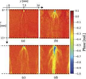
Figure 5. Obtained phase shift variations in humid air with Vp = 26.6 kV for (a) t = 1 μs, (b) t = 10 μs, (c) t = 100 μs, and (d) t = 1000 μs.
Download figure:
Standard image High-resolution image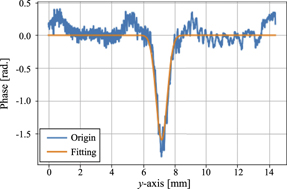
Figure 6. Fitting example for phase shift variations. The increase in phase around y = 0.5 and 14 mm are derived from the adjacent streamers.
Download figure:
Standard image High-resolution image3. Results
Figure 7 shows the z-axis distribution of the local density (ρ) obtained from the fitting. The standard errors are marked using error bars; however, the bars are small, and thus, hidden by the corresponding symbols in figure 7. Evidently, immediately after (1 μs) the discharge, the density just below the needle was approximately 70%; however, it decreased to approximately 25% at 10 μs. After the discharge, the density continuously decreased until approximately 100 μs at all the z-positions; however, the decrease in density near the needle was gradual. At 1000 μs, the density increased at z < 2 mm. Locally, the gas temperature near the needle was high [26]; accordingly the rate of gas diffusion was also increased near the needle. This may have resulted in the observed faster diffusion and lower temperatures at z < 2 mm than at other z-positions. Alternatively, because the needle electrode was made of metal and had a large heat capacity, it is possible that only the needle electrode was rapidly cooled, thereby reducing the gas temperature.
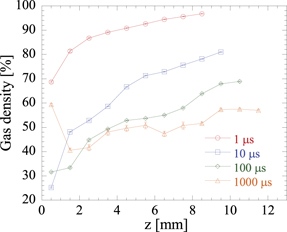
Figure 7. Axial distribution of gas density after discharge in humid air with Vp = 26.6 kV.
Download figure:
Standard image High-resolution imageAs shown in figure 7, the gas density changed considerably specifically near the needle. To understand the basic mechanism of the discharge-induced change in the density (increases or decreases), we focused on the gas-density change at z = 6–7 mm near the centre of the needle; this prevented the observation of specific locations, such as the anode or cathode. Figure 8(a) shows the change in gas density at z = 6–7 mm for different Vp values in humid air, and figure 8(b) shows the full width at half maximum (FWHM) calculated from the Gaussian fitting parameter b as  . Figure 8(a) shows that the gas density decreased immediately after the discharge and continued to decrease until 1000 μs. In addition, the decrease in the gas density was always larger at a higher voltage, from the time of discharge to 10000 μs. Similarly, figure 8(b) indicates that the FWHM of the density distribution before 1000 μs was large at high voltages, thus indicating that the diameter of the streamer increased with increasing voltage. Notably, the temporal variation of the FWHM exhibited a discontinuity at approximately t = 10 μs (where t is time). This was caused by the pressure wave generated near the needle, as observed in figure 5(b). The time constant of the pressure wave propagation in the axial direction was estimated to be approximately 0.006/340 = 17.6 μs, based on the sound velocity (340 m s−1) and measurement position (z = 6 mm). This discontinuity was caused by the assumption that the radial distribution of the density is Gaussian; therefore, we cannot say that it accurately represents the streamer channel diameter. However, the standard error of the FWHM was as small at t = 10 μs as at other points, and the reproducibility of the pressure wave propagation and its effect on the channel diameter was high. The FWHM increased after 1000 μs, thus suggesting that the diffusion was pronounced, and the gas density (figure 8(a)) decreased accordingly.

Figure 8. (a) Temporal variations in gas density at z = 6–7 mm in humid air for different Vp values and (b) corresponding FWHM plots of channel diameters calculated from Gaussian fitting parameter b.
Download figure:
Standard image High-resolution imageTo relate the change in gas density to the discharge energy, the relationship between the minimum density and discharge energy was obtained from figures 2(b) and 7(a). The results are shown in figure 9. In the range of low-discharge energies (Vp = 17 and 21.2 kV), the gas density decreased proportionally to the discharge energy, whereas at Vp = 26.6 kV, the gas density showed deviations from the line of proportionality. This could be possibly attributed to the increase in the gas temperature and decrease in the density owing to the fact that the discharge accelerated the diffusion rate of the molecules, which in turn accelerated the increase in the gas density.
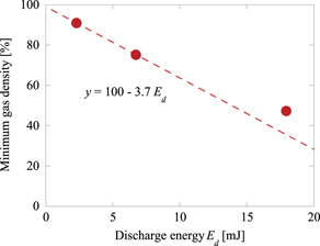
Figure 9. Dependence of minimum gas density on discharge energy in humid air.
Download figure:
Standard image High-resolution imageTo investigate the effects of different background gases on the gas-density changes after the discharge, the applied voltage was set to Vp = 17 kV, and the gas density and FWHM were measured at different gas compositions. The results are shown in figure 10. Figure 10(a) shows that the decrease in the gas density was larger in N2 and humid gas than in air and dry gas. The decrease in density was especially substantial after a few tens of microseconds in humid-N2 conditions. Conversely, the FWHM (figure 10(b)) did not show any change under different background gases. This suggests that the change in gas density inside the discharge channel was not due to differences in the channel diameter or diffusion rate but due to differences in the energy relaxation processes depending on the gas composition.
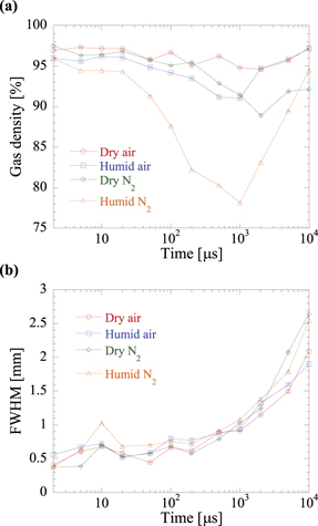
Figure 10. (a) Temporal variations in gas density at z = 6–7 mm for different background gas compositions with Vp = 21.2 kV and (b) corresponding FWHM plots of channel diameters.
Download figure:
Standard image High-resolution imageFor a more substantive discussion, the changes in gas density and FWHM were compared by keeping the discharge energy same, i.e. 6.8 mJ, for each background gas. The results are shown in figure 11 for N2 and air. For both dry air and dry N2, the density became minimum at 2000 μs and then increased. In humid-air and humid-N2 conditions, the gas densities had almost equal minimum values at 500 and 1000 μs. Figure 11(b) shows the FWHM on a log–log scale. The FWHM in air was larger than that in N2 until 1000 μs; subsequently, these FWHMs started showing tendencies that were similar to those of the diffusion length, whose slope is expressed as  , where t is time. This indicates that the FWHMs after 1000 μs were controlled by the diffusion under all conditions. In practice, the diffusion length is expressed as
  , where D is the diffusion coefficient. In our case, the actual value of D was expected to vary with time and space because the gas temperature in the streamer channel was not uniform; it was much higher than the background temperature. This time variation in D is considered to be the reason why the FWHM within 1000 μs did not show the slope ∼
  .
.
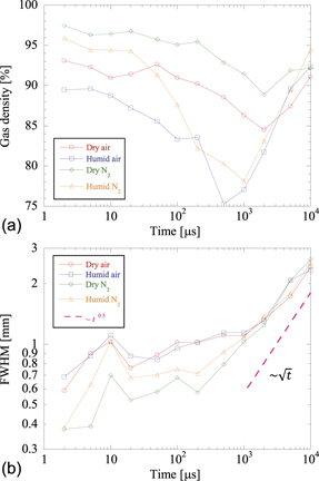
Figure 11. Temporal variations in gas density at z = 6–7 mm for different background gas compositions with the same discharge energy and (b) corresponding FWHM plots of channel diameters. The dashed line indicates the slope  .
.
Download figure:
Standard image High-resolution imageThese results will be discussed in more detail in the discussion section.
4. Discussion
In pulsed streamer discharges in air, the gas temperature is known to increase in two stages. The first stage is caused by the energy relaxation of electronically excited molecules produced during the discharge [27] and the second stage is due to the energy relaxation of vibrationally excited molecules after the discharge [2, 28]. Because the energy relaxation of electronically excited species proceeds in the order of microseconds, the decrease in gas density measured in this study at t = 1–2 μs is possibly due to the temperature increase in the first stage. This rapid temperature increase causes the pressure wave generation observed at figure 5(b). On the other hand, because the energy relaxation of vibrationally excited molecules is known to proceed in the order of 10–1000 μs, the observed decrease in gas density at time constants after 10 μs may be due to the vibrational energy relaxation. In addition, the increase in gas density in the order of 0.1–10 ms may be due to molecular diffusion [29]. The ratio of the energy distribution of the electronically excited species and that of the vibrationally excited species could not be elucidated in this study. Popov [27] showed that the energy distribution in plasma depends on E/N, and in a streamer discharge, a significant amount of this energy is utilized to cause electron excitation and ionisation of the gas. This leads to a more efficient and fast energy thermalisation. However, in the pulsed streamer discharge, a large amount of the discharge energy goes to the secondary streamer, whose E/N is known to be 2–3 eV [30, 31]. Therefore, a significant amount of the discharge energy is expected to store in the vibrational energy mode of molecules.
In this section, we focus on the differences in the vibrational energy relaxation process between different gases by discussing the gas-density change characteristics using a zero-dimensional reaction simulation model, which was previously developed by our group [28], for the vibrationally excited molecules of N2, O2, and H2O.
Table 1 presents the reactions that were considered in the simulation. In the simulation, the vibrational levels of H2O (ν1, ν2, ν3) can be classified as equilibrated stretching (ν1, ν3) levels and a bending (ν2) level. The stretching levels (ν1, ν3) are neglected because the rates of the V–V processes for O2 and N2 are negligibly slow [32, 33]. The higher vibrational level of H2O (ν2 > 1) is also neglected because there is no dominant path for the ν2 > 1 excitation owing to the extremely rapid relaxation of the H2O (010) process (R3 in table 1). Therefore, for the vibrational states of H2O, only the bending levels of ν2 = 0 and 1 are considered. For O2(v) and N2(v), only v ⩽ 8 is considered because highly excited molecules (v > 8) have minor effects on the vibrational-to-translational (V–T) and vibrational-to-vibrational (V–V) processes. This is because the densities of v > 8 molecules are relatively small in atmospheric-pressure pulsed streamer discharge [15]. The temporal evolutions of the vibrationally excited O2, N2, and H2O densities are numerically calculated by solving differential equations, where the rate coefficients are calculated in each time step. The method for calculating the rate coefficient of the reactions shown in table 1 is described in detail in our previous paper [28].
Table 1. Vibration-to-translation (V–T) and vibration-to-vibration (V–V) reactions considered in our simulation. Here, v and w are vibrational quantum numbers.
| V–T processes | |
|---|---|
| R1 | O2 (v = 1) + O2↔ O2 (v = 0) + O2 |
| R2 | N2 (v = 1) + N2↔ N2 (v = 0) + N2 |
| R3 | H2O (010) + H2O ↔ H2O (000) + H2O |
| R4 | O2 (v = 1) + N2↔ O2 (v = 0) + N2 |
| R5 | N2 (v = 1) + O2↔ N2 (v = 0) + O2 |
| V–V processes | |
|---|---|
| R6 | O2 (v = 1) + O2 (w = 0) ↔ O2 (v = 0) + O2 (w = 1) |
| R7 | N2 (v = 1) + N2 (w = 0) ↔ N2 (v = 0) + N2 (w = 1) |
| R8 | N2 (v = 1) + O2 (w = 0) ↔ N2 (v = 0) + O2 (w = 1) |
| R9 | O2 (v = 1) + H2O (000) ↔ O2 (v = 0) + H2O (010) |
| R10 | N2 (v = 1) + H2O (000) ↔ N2 (v = 0) + H2O (010) |
In the formulation of the kinetic energy exchange between the translational, rotational, and vibrational levels of molecules, we assumed the translational and rotational energies stored per molecule to be equal to their classical values of  for N2 and O2 and
  for H2O [34], where k is the Boltzmann constant, and T is the translational temperature. This assumption was made because the translational and rotational temperatures are instantaneously equilibrated in air discharge [11]. The conservation law of translational, rotational, and vibrational energies can be written as [11]
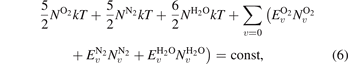
where NM is the number density of molecule M,  is the density of the vth vibrational level of molecule M, and
  is the energy of the vibrational level v. Vibrational relaxation leads to an increase in the translational temperature, as described by equation (6).
In addition to the effects of the V–V and V–T reactions, the effect of thermal diffusion is substantial because the time constants of the diffusion and V–T reactions are comparable [12] in the streamer discharge at atmospheric pressure. Therefore, we added the effect of diffusion with the use of the time constant of diffusion, td, which was estimated from the results shown in figure 10(b). The constant was found to be approximately 6.8 ms, independent of the gas species. The change in the gas temperature owing to diffusion was included based on the Newton's law of cooling. Using this, a temporal variation in the translational temperature can be written as follows,

where  is the change in the gas temperature caused by the vibrational relaxation processes calculated in each time step using equation (6), T0 is the background gas temperature (assumed to be 300 K), and td is the diffusion time constant (6.8 ms).
The temporal evolutions of the gas temperature were calculated and compared with the experimental results shown in figure 11. For the calculation, the following assumptions were postulated:
- (a)The gas pressure was assumed to relax instantaneously to the atmospheric pressure, and the gas temperature changed according to the ideal gas state equation.
- (b)
- (c)The initial gas temperature was estimated from the experimentally obtained gas density at t = 10 μs. This density was calculated using the ideal gas state equation subject to the assumption that the gas pressure reached the atmospheric pressure.
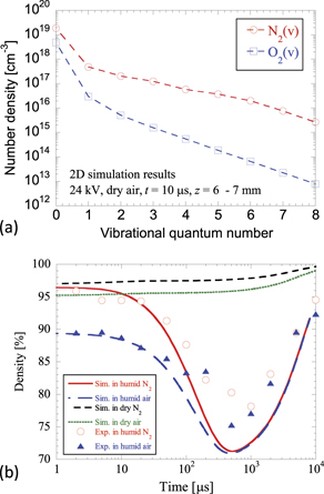
Figure 12. (a) Vibrational distributions of N2(v) and O2(v) at z = 6–7 mm, obtained from the 2D streamer discharge simulation results [2]. The simulation was performed using conditions similar to those in the experiment. (b) Simulation results of gas-density variations. The experimental results obtained in humid-air and humid-N2 conditions are also plotted for comparison.
Download figure:
Standard image High-resolution imageThe gas pressure reduced almost in proportion to the speed of sound. The time constant of the speed of sound was approximately ![$\frac{{d}_{\mathrm{s}}}{{v}_{\mathrm{s}}}\sim \frac{0.5{\times}2\enspace [\mathrm{m}\mathrm{m}]}{347\enspace [\mathrm{m}\enspace {\mathrm{s}}^{-1}]}=$](https://content.cld.iop.org/journals/0963-0252/30/9/095007/revision2/psstac1defieqn14.gif) 2.9 μs, where vs is the speed of sound at T = 300 K, and ds is the diameter of the streamer channel estimated from the experimental results shown in figure 10(b). The estimation of the time constant of the pressure relaxation from the time constant of the speed of sound indicated that assumption (a) was valid, at least for the data over several microseconds after the discharge. For assumption (b), we used the vibrational populations of O2 and N2 previously simulated using the 2D streamer simulations in dry air at atmospheric pressure [2]; this simulation was performed using conditions similar to those used in the present experiment, i.e. H2O (2.3%)/O2 (19.5%)/N2, and H2O (2.3%)/N2 at atmospheric pressure were used in the simulations. The 2D simulation was performed in dry-air conditions. Moreover, the discharge in N2 and in humid gases have different parameters because of the differences in the ionisation and photoionisation terms [35]. However, for simplicity, we assumed that the vibrational populations of O2 and N2 were the same as those in humid-air conditions. In addition, we assumed that the vibrational populations of N2 in humid-N2 and dry-N2 conditions were equivalent to 5/4 times the vibrational populations of N2 under dry-air conditions as long as the discharge energies were the same. Because the experimental results shown in figure 11 were obtained using the same discharge energy for different background gas species, we performed the simulations with the same conditions as those shown in figure 11, and compared the results. Assumption (c) was based on assumption (a). For example, the gas density at t = 10 μs in humid N2 conditions in figure 11 is 95%, and the initial gas temperature was assumed to be
2.9 μs, where vs is the speed of sound at T = 300 K, and ds is the diameter of the streamer channel estimated from the experimental results shown in figure 10(b). The estimation of the time constant of the pressure relaxation from the time constant of the speed of sound indicated that assumption (a) was valid, at least for the data over several microseconds after the discharge. For assumption (b), we used the vibrational populations of O2 and N2 previously simulated using the 2D streamer simulations in dry air at atmospheric pressure [2]; this simulation was performed using conditions similar to those used in the present experiment, i.e. H2O (2.3%)/O2 (19.5%)/N2, and H2O (2.3%)/N2 at atmospheric pressure were used in the simulations. The 2D simulation was performed in dry-air conditions. Moreover, the discharge in N2 and in humid gases have different parameters because of the differences in the ionisation and photoionisation terms [35]. However, for simplicity, we assumed that the vibrational populations of O2 and N2 were the same as those in humid-air conditions. In addition, we assumed that the vibrational populations of N2 in humid-N2 and dry-N2 conditions were equivalent to 5/4 times the vibrational populations of N2 under dry-air conditions as long as the discharge energies were the same. Because the experimental results shown in figure 11 were obtained using the same discharge energy for different background gas species, we performed the simulations with the same conditions as those shown in figure 11, and compared the results. Assumption (c) was based on assumption (a). For example, the gas density at t = 10 μs in humid N2 conditions in figure 11 is 95%, and the initial gas temperature was assumed to be  K. The differences in the initial gas temperatures of different gases were caused by the differences in the generated discharge and energy relaxation processes of the excited molecules produced in the discharge channel [10, 27]. To minimise the induced fast expansion of the gas during the initial stage of the flow field formation, such as the shock wave propagation and channel expansion/contraction, the initial gas temperature was determined by the gas density at t = 10 μs. Assumptions (a)–(c) are very simple and approximate; however, they are convenient for investigating the fundamental characteristics of the vibrational relaxation phenomenon, as proved in our previous study.
Figure 12(b) shows the simulation results. The experimental data for the humid-air and humid-N2 conditions shown in figure 11 are also plotted for comparison. As shown in figure 12(b), the simulated densities in humid-air and humid-N2 conditions first decreased because of the gas heating induced by the vibrational relaxation, and then increased because of diffusion. These findings are qualitatively in good agreement with the experimental results, although the minimum densities were slightly lower. Conversely, the simulation results for dry-air and dry-N2 conditions were different from the experimental results. The simulated densities in dry air and dry N2 did not show any decrease; they increased because of diffusion. This is because the rate of vibrational relaxation in dry conditions is slower than that of diffusion. Figure 13 shows the simulated vibrational temperatures of N2 in (a) dry-air and (b) humid-air conditions. The vibrational temperatures were described by defining two vibrational temperatures based on a previous study: Tvib(01), which characterises the levels v = 0 and v = 1; and Tvib(1v), which characterises the levels v ⩾ 1 [15]. In both dry-air and humid-air conditions, Tvib(01) increased and Tvib(1v) decreased until approximately 100 μs because of V–V relaxation. After 100 μs, the vibrational temperatures in humid air gradually relaxed and decreased to the gas temperature. However, the vibrational temperatures in dry air remained higher than the energy relaxation temperature between the gas and vibrational temperatures, even at 10 000 μs. These simulation results clearly showed the effects of humidity on the vibrational relaxation after the discharge.

Figure 13. Simulated gas temperature and vibrational temperatures of N2 under (a) dry-air and (b) humid-air conditions. Tvib(01) indicates the vibrational temperature determined by N2 (v = 0) and N2 (v = 1) densities, and Tvib(1v) indicates the vibrational temperature determined by the N2 (v ⩾ 1) densities.
Download figure:
Standard image High-resolution imageFrom these results, we can infer the following facts:
- The gas-density variations after streamer discharge in humid conditions can be explained by the acceleration of the vibrational relaxation of water molecules.
- The gas-density variations after streamer discharge in dry conditions cannot be explained by the reactions listed in table 1.
Previous reports have shown that the humidity in air accelerates the rate of vibrational relaxation, thus resulting in gas heating during the post-discharge period of streamer discharges [36, 37]. In addition to the previous reports, this study shows that the acceleration of the vibrational relaxation can be observed even in humid-N2 conditions and can be explained by the acceleration of vibrational relaxation through water molecules, as shown in figure 12. Conversely, the vibrational relaxation in dry conditions cannot be explained by the reactions listed in table 1.
In general, the dried gas from a gas cylinder may contain impurities as it passes through the gas line. The effect of residual H2O was numerically analysed in the simulation, and the corresponding results are shown in figure 14. These results indicate that to simulate the same amount of gas density decrease as in the experiment, it is necessary to include at least several hundred ppm of H2O in both O2 (20%)/N2 and N2 conditions. However, in our experiment, dry gas was constantly supplied to the discharge reactor from the gas cylinder at a flow rate of 2 L min−1. Furthermore, we ensured that the H2O number density remained less than 100 ppm at the inlet of the discharge reactor. Thus, it is expected that the influence of the residual water molecules on the results should be small.

Figure 14. Simulation results of gas-density variations for (a) O2 (20%)/N2 and (b) N2 conditions at different H2O contamination in the range of 10–1000 ppm. The experimental results obtained in dry-air and dry-N2 conditions are also plotted for comparison.
Download figure:
Standard image High-resolution image
However, we believe that this difference between the experimental and simulation results in dry conditions was observed possibly because the effects of vibrational relaxation through atomic N and O were not considered in the simulations. It has been reported that V–T relaxation by N and O radicals is important in some cases [11]. The V–T process of O2(v)–O has been investigated theoretically and experimentally [38, 39]. The reaction time constant of O2(v)–O with an O concentration of 1000 ppm was approximately 12.8 μs [38] at 300 K. However, the vibrational energy stored in N2(v) was considerably higher than that stored in O2(v), and the effect of the V–T reactions of O2(v) on gas-density variations may be low. For the V–T reactions of N2(v) by O and N atoms, the time constant of N2(v)–O with an O concentration of 1000 ppm was approximately 12 800 μs [11] at 300 K; this constant seems to be smaller than the diffusion time constant. The effects of N on the V–T reactions are difficult to estimate because experimental data on N concentration after streamer discharge are not available. In any case, it is difficult to elucidate the mechanism of density variations after streamer discharge in dry conditions solely based on the results obtained in this study. This is because the O and N densities were not measured simultaneously in this study. For the precise evaluation of the vibrational relaxation in dry conditions, it is desirable to measure the translational temperature, vibrational temperatures of O2 and N2, and density of atomic O and N.
5. Conclusions
In this study, we used the Mach–Zehnder interferometry to measure the gas density quantitatively after streamer discharge, and analysed the mechanism of the density variation after the discharge in different background gases. The experimental results showed that the density first decreased because of vibrational relaxation and then increased because of diffusion. Numerical simulation results showed the effects of humidity on vibrational relaxation. Conversely, the gas-density variations obtained under dry-air and dry-N2 conditions could not be explained by the V–V and V–T reactions considered in this study possibly because the V–T reactions with O and N atoms were ignored owing to the lack of experimental data. For a precise understanding of the vibrational relaxation in dry conditions, it is desirable to measure the gas density (or temperature) as well as the O and N atom densities.
Acknowledgments
This work was partially supported by JSPS KAKENHI under Grant Nos. 26889004, 16K14207, and 18H01417.
Data availability statement
The data that support the findings of this study are available upon reasonable request from the authors.