

Abstract
Kinetic effects and nonlinear characteristics caused by multi-dimensional effects in capacitively coupled plasma (CCP) devices are reported using particle-in-cell (PIC) Monte-Carlo collision simulations. Many PIC simulations so far are limited to one-dimensional (1D) dynamics due to computational load, and the nonuniformity occurring in a direction parallel to the electrode cannot be reflected consequently. A two-dimensional (2D) PIC–MCC simulation based on a graphics processing unit is utilized to observe the variations in the spatial distribution that cannot be dealt with by 1D simulations. This simulation considers the pressure regime of the nonlocal electron kinetics. Contrary to the expectation that motions in the vertical direction to the electrode in a CCP dominate most of the particle dynamics, it was observed that electron heating in the horizontal direction around the electrode edge plays an important role. Accordingly, the change in the spatial distribution between the center of the CCP equipment and the peripheral region of the electrode edge has been analyzed by phase-resolved electron flux and power deposition to understand the principle of the formation of spatial nonuniformity.
Export citation and abstract BibTeX RIS
1. Introduction
Many studies on the nonuniformity phenomenon have been conducted through plasma characteristic analyses to increase the manufacturing yield of semiconductors and displays. Several studies on the methods and results of experimentally measuring capacitively coupled plasma (CCP) devices using a Langmuir probe or cut-off probe have also been conducted [1, 2]; however, there are evident disadvantages, such as probe contamination and measurement constraints, in which a particular method can generally measure only limited cases. In addition, the devices used in the industry are difficult to measure because a probe itself perturbs plasmas. To overcome this problem and observe various kinetic factors, many studies have been conducted using one-dimensional (1D) particle-in-cell (PIC) simulations, followed by comparing their results with experimental results. However, the equipment used in the actual process comprises complex structures; consequently, 1D simulations cannot accurately reflect these structures or their boundary conditions. Therefore, only limited analyses are possible, and the accuracy is particularly low for CCP devices.
Although many cases of two-dimensional (2D) fluid simulations are available, PIC simulations are required because of the limitations of fluid simulations assuming electron energy distributions, which are attributed to the nonlinear kinetic effect of CCP discharges [3–6]. In particular, when nonlocal kinetics are considered, a PIC simulation is required to accurately calculate the time-dependent electron heating and transport in the CCP chamber because the regions are different where electrons obtain and consume energy. In nonlocal kinetics, the energy distribution function of electrons generally has a two-temperature profile [7–9]. However, due to the computational load and difficulty of parallelization of the PIC simulation, most results of 1D simulations have been used [10–24]. As such, the electron heating and transport in the radial direction in CCP using 2D PIC simulations have been rarely studied [25–28].
The process of optimizing control parameters by comparing the 2D simulation results with regard to the driving conditions of the actual process equipment is essential. However, the full 2D PIC simulation is not practical for parameter study as the computation time per case is too long. The parallelized graphics processing unit (GPU)-based 2D simulation used in this study [29] significantly shortened the computational time to a steady-state per case by utilizing a more significant number of cores than that used in a CPU-based computation. It shortens the simulation time to reach a steady-state in approximately a few days [28–31], which took several months in the past. Unlike fluid simulations, the PIC simulation has the advantage of observing the velocity distribution by calculating the exact kinetic energy of each particle [8, 9, 32, 33]. Furthermore, there is no limitation for analyzing the electrodynamics at low pressure with a large Knudsen number, as the mean free path of electrons is larger than the plasma system size [8].
In this study, we analyze the 2D spatial distribution affected by the asymmetry of plasma motions using a 2D GPU–PIC simulation, which overcomes the limit of 1D PIC simulations. We compare the effect of the 2D particle kinetics in a nonlocal kinetics regime. The remainder of the paper organized as follows: in section 2, simulation conditions are specified. In section 3, the simulation results are presented, and finally, the conclusions are provided in section 4.
2. PIC simulation conditions
The considered structure of the CCP equipment used in this study is shown in figure 1. The radius (actually half of the x-directional length) is varied from 6 cm to 16 cm. We used 2D rectangular geometry instead of cylindrical geometry in this study. As indicated in table 1, the grid size and the time step were selected considering the Courant–Friedrichs–Lewy condition, the Debye length, and plasma frequency to satisfy the spatiotemporal resolution. The CCP chamber is symmetric at x = 0 by applying the Neumann boundary condition. In many cases, the upper and lower electrodes are asymmetrically configured to control the flux and energy of ions toward the wafer by controlling the thickness of the lower sheath with the self-bias voltage. However, in this case, we chose the symmetric geometric to exclude these effects and focus on particle dynamics without self-bias. NP2C in table 1 is defined as the number ratio of the real particles to one computational particle. It is about 3 × 10⁶ for case 4. Typically, we keep more than 20 computational particles per cell at a steady state. If the number is too small, the increasing numerical noise induces numerical heating. If the number is too large, the computational load is very heavy. The secondary electron emission by ion bombardment and electron reflection at the boundary are also excluded for the same reason as described above, although these options are implemented in the simulation code.
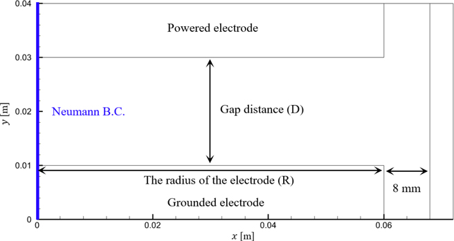
Figure 1. Schematic of the 2D GPU–PIC simulation.
Download figure:
Standard image High-resolution imageTable 1. GPU-PIC simulation condition.
| Simulation domain | 7.2, 11.2, or 17.2 (cm) × 4 (cm) |
| Gas type | Argon |
| Time step | 14.4 (ps) |
| Grid size | ∆x = ∆y = 0.2 (mm) |
| NP2C | 2 × 10⁶ |
| Gas pressure | 100 (mTorr) |
| Driving frequency | 13.56 (MHz) |
| Input voltage | 100 (V) |
Table 2 lists up the cases observed in this study. To mimic the 1D condition, case 1 adopted the Neumann boundary condition to both vertical sides as designated in figure 2(b). Cases 2–4 are with the variation of the electrode radius of 6, 10, and 16 cm. The range of gas pressure for the industrial application of CCPs is quite broad, from a few mTorr for etching to a few Torr for deposition processes. Our primary purpose is to investigate the effect of nonlocal kinetics on the spatial nonuniformity caused by the energy relaxation process. At 100 mTorr, the energy relaxation length of electrons is larger than the gap distance. The transition of the local and nonlocal kinetics appears around 200 mTorr for the given geometry. The voltage applied to the electrode was fixed at 100 V. The simulations were performed under the condition that the external capacitance is sufficiently large; that is, self-bias could be neglected in particular.
Table 2. List of the simulation cases for the directional and 2D spatial profiles in this study.
| Case No. | Pressure (mTorr) | R (cm) | D (cm) | Sidewall condition |
|---|---|---|---|---|
| 1 | 100 | 6 | 2 | Neumann |
| 2 | 100 | 6 | 2 | Grounded |
| 3 | 100 | 10 | 2 | Grounded |
| 4 | 100 | 16 | 2 | Grounded |
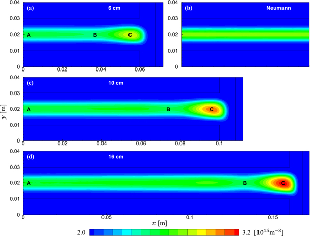
Figure 2. The time-averaged spatial profile of the electron density for (a) case 2, (b) case 1, (c) case 3, and (d) case 4.
Download figure:
Standard image High-resolution image3. Computational results and analysis
After the plasma behavior reached a steady-state, time-averaged 2D spatial distributions were observed for 10 radiofrequency (RF) cycles. To describe the profiles of each parameter in a specific area where significant changes occur among spatial distributions, regions A, B, and C were marked in the figures.
Figure 2 shows the spatial distribution of the time-averaged electron density. Unlike the uniform radial profile in the 1D condition shown in figure 2(b), the spatial distributions of cases 2, 3, and 4 show nonuniform radial profiles having the maximum value in region C near the electrode edge. Moreover, in region B, the density significantly decreases to form a saddle point. The distances from the electrode edge to regions C and those between regions B and C are almost the same for all the cases. The density becomes uniform as it goes close to region A.
Figure 3 shows the 1D plot of the time-averaged electron density in the x-direction at y = 0.02 m. Unlike the uniform density of case 1 indicated by the dashed lines in figure 3(a), the spatial nonuniformity of the 2D simulation results is large, and the tendency becomes larger as the length of the electrode increases. Due to the overall plasma transport in the horizontal direction, the density at the center becomes smaller than that of the 1D simulation result. However, the density in region C increases larger than that of the 1D simulation result due to the enhanced ionization by the strong electric field at the electrode edge. The difference in the electron densities between regions B and C increases as the electrode length increases. The decrease in the electron density in region B is caused by a nonlocal effect, which will be described in detail later by analyzing it together with other parameters.

Figure 3. The time-averaged spatial profiles of (a) the electron density at y = 0.02 m and (b) the magnified electron and ion densities near the rhs boundary.
Download figure:
Standard image High-resolution imageFigure 4 shows the spatial distribution of plasma potential averaged for 10 RF periods. Because the voltage rather than the power is fixed as the electric potential boundary condition, the maximum plasma potential did not significantly change as the electrode length increases. However, in figure 4(b), representing the 1D case, it is uniform in the x-direction, whereas the other cases show the difference in the spatial distribution in the x-direction. In figures 4(a), (c) and (d), the potential is always maximized in region C, where sheaths exist toward the sidewall as well as the top and the bottom electrodes. In region B, the time-averaged potential gradient in the y-direction is relatively smaller than that in region C, and it has a saddle point shape in figure 4(c). It results from the decrease in the density of charged particles in region B, as observed in figure 2.
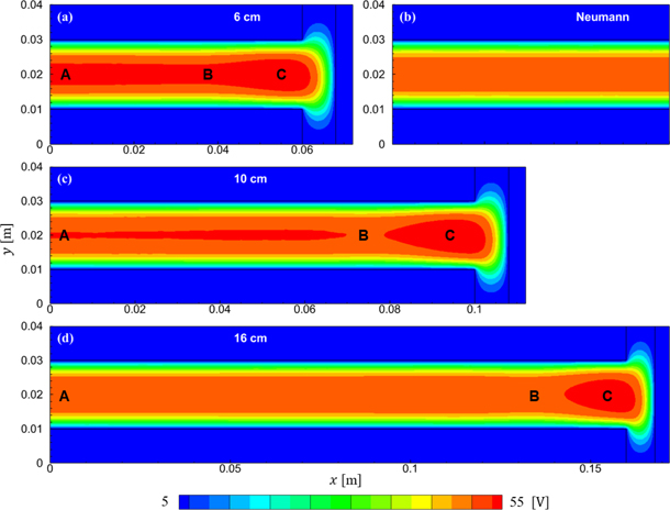
Figure 4. The time-averaged spatial profile of the plasma potential for (a) case 2, (b) case 1, (c) case 3, and (d) case 4.
Download figure:
Standard image High-resolution imageFigure 5 shows the spatial distribution of potentials in different phases during one RF period for case 4. T is the period of the sinusoidal voltage waveform, which is applied on the powered electrode at the top. At phase 0, shown in figure 5(a), the potential of the top electrode is changing from negative to positive, and the potential in region A is maintained larger than that in region B. At phase T/2, shown in figure 5(c), this tendency is reversed, and the potential value in region A becomes smaller than that in region B. In contrast, the potential difference between regions A and B is very small in phases T/4 and 3T/4. Overall, the potential in region C is always larger than that in region B. Therefore, the x-direction electric field in the discharge space changes with time as a higher harmonics waveform. In particular, figures 5(b) and (d) show that the electric field is relatively uniform in the x-direction from region A to region B. However, in figures 5(a) and (c), the electric field is strong because the potential gradient in the x-direction is remarkable when the driving voltage transitions from the positive cycle to the negative cycle (phase T/2) and the opposite point (phase 0). Therefore, electron transport crossing from the center to the sidewall plays an essential role. Although this phenomenon is not included in the 1D simulation, it is considered an important factor in understanding the cause of nonuniformity.
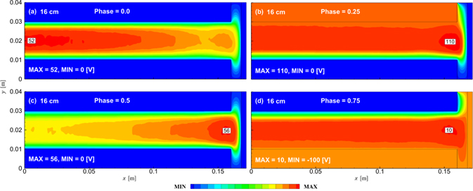
Figure 5. The spatial profile of the plasma potential of case 4 for different phases at (a) 0, (b) T/4, (c) T/2, and (d) 3T/4.
Download figure:
Standard image High-resolution imageFigure 6 shows the time-averaged electron flux in the x-direction (left) and y-direction (right). As shown in figure 6(b), the spatial change of the x-directional electron flux is negligible at the level of localized noise in case 1. However, with the presence of the sidewall, there are clear layers in the spatial distribution of the x-directional electron flux. Because of the Neumann boundary condition at x = 0, the electric field in the x-direction is negligible in region A, which is at the same noise level as shown in figure 6(b). However, there are distinguished time-averaged electron flows in figures 6(a), (c) and (d) between regions A and B, and the magnitude becomes more substantial with a more extended electrode. At the bulk-sheath boundary near the powered electrode (0.025 m < y < 0.028 m), the electron flux moves in the inward x-direction. In contrast, the x-directional electron flux has an outward direction in the bulk center area between regions A and B for 0.016 m < y < 0.024 m. Between regions B and C, the time-averaged x-directional electron flux shows inward direction if y > 0.016 m following the negative density gradient. That is to say, the time-averaged electron flux follows the diffusion term in the bulk plasma between region B and C. Except for this location, however, the time-averaged value of the x-directional electron flux differs from the profile of the negative density gradient.
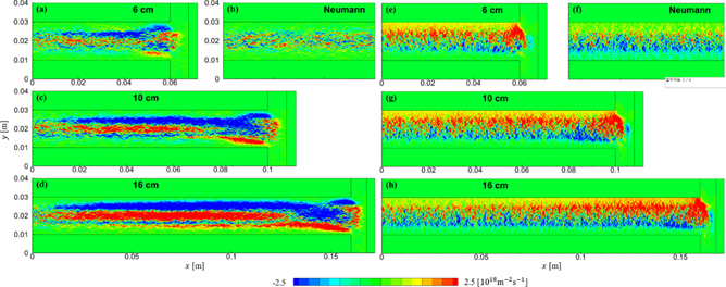
Figure 6. The time-averaged spatial profiles of (a), (b), (c), (d) the electron flux in the x-direction and (e), (f), (g), (h) y-direction with the variation of the electrode length for cases 1–4.
Download figure:
Standard image High-resolution imageFor the electron flux in the y-direction, the overall shape is almost the same for figures 6(e), (g) and (h) and much stronger than that of the 1D case shown in figure 6(f) because the plasma potential is larger for the 2D cases. The electron flux in the y-direction at region C always larger than that at region A due to the increased electron density in region C. The y-directional electron fluxes in the regions above and below y = 0.02 m are opposite, but the positive direction is more dominant. In region C, the electron flux in the positive y-direction is more dominant because the temporal electric field is not vertically symmetric due to the geometric effect (larger grounded area than the powered electrode area).
Figure 7 shows the y-directional slices of the phase-resolved electron fluxes with two different electrode lengths, 6 cm (case 2) and 16 cm (case 4). The first row is the electron flux in the x-direction [(a)–(d)], and the second row is the electron flux in the y-direction [(e)–(h)] for the two RF periods. In region A, the electrons move randomly in the x-direction because the horizontal electric field is close to zero in both cases. In the y-direction, the positive and negative phases of the electron flux are clearly distinguished according to the sheath expansion and contraction phase. In region B, however, the x-direction electron flux also clearly oscillates in both cases. The fluxes in regions A and B shown in figure 6 are the time-averaged value of the oscillations shown in figure 7. Therefore, the maximum value of the scale shown in figure 6 is smaller by 1/20 compared with that in figure 7. Comparing figures 7(a), (c) and (g), we found that there is not much difference in region A for case 2 and case 4. However, the x-directional electron flux in region B is much larger in case 4 than in case 2, as shown in figures 7(b) and (d). As shown in figure 3(a), the electron densities in regions A and B are similar for both cases. Also, the density difference in region B is less than 10% for cases 2 and 4. The reason for the large fluctuation of the x-directional electron fluxes in region B with a longer electrode is not the increase of electron density but enhanced electron heating in region B, which will be explained in figures 8 and 9.
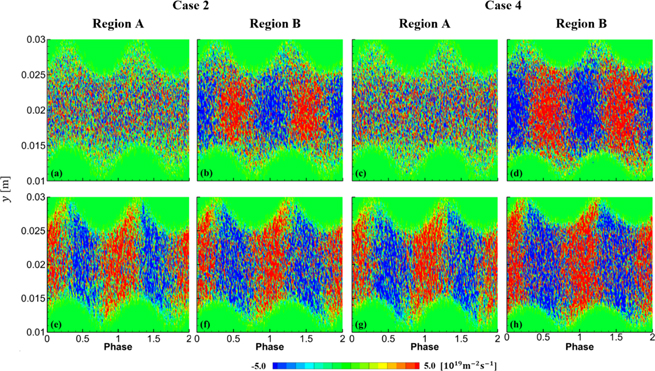
Figure 7. Phase-resolved profile of the electron flux in the x-direction (first row) and y-direction (second row) at region A (x = 0) and region B (x = 3.6 cm for case 2 and x = 13.2 cm for case 4).
Download figure:
Standard image High-resolution image
Figure 8. The time-averaged spatial profile of the electron power density for (a) case 2, (b) case 1, (c) case 3, and (d) case 4, as well as the decomposition of the power density in (e) the x-direction and (f) in the y-direction.
Download figure:
Standard image High-resolution image
Figure 9. Phase-resolved profile of the electron power density in the x-direction (first column), y-direction (second column), and the total (third column) at region A (x = 0) and region B (x = 3.6 cm for case 2 and x = 13.2 cm for case 4).
Download figure:
Standard image High-resolution imageFigure 8 shows the spatial distribution of the time-averaged electron power density. Under the pressure condition of 100 mTorr that maintains nonlocal kinetics, it is well known that the spatial profile of the electron power absorption has the maximum value in the bulk-sheath boundary [8] with the help of the electron acceleration by the expanding sheath. Figure 8(b) presents the 1D condition showing spatial uniformity in the x-direction. With a 2D boundary, strong electric fields near the right wall and around the electrode edge generate stronger heating than stochastic heating in the sheath region. In particular, heating in region B is especially apparent in figures 8(c) and (d), which increases as the electrode length increases because electrons are heated while flowing horizontally as the potential changes in the region. Figures 8(e) and (f) shows the time-averaged profiles of the electron power absorption for case 4 in the x- and y-direction, respectively. The electron power absorption in the x-direction is prominent in a wide range from x = 7 cm to x = 15 cm as shown in figure 8(e). Note that the scale of the contour is magnified twice only in figure 8(e) compared with others. The maximum electron heating is spotted at the corner of the bottom ground electrode in the y-direction by geometric effect, while electron cooling happens at the corner of the top electrode, as shown in figure 8(f).
Figure 9 shows the time-resolved electron power deposition in regions A and B for two different electrode lengths. The first row shows the x-directional heating, the second row shows the y-directional heating, and the third row shows the total. In the y-direction power deposition, the heating and cooling phases are clearly distinguished by the sheath oscillation in both regions A and B. As the length of the electrode increases from case 2 to case 4, the magnitude increases, but there is no significant difference in the patterns in regions A and B. In contrast, the absorption of electron energy in the x-direction does not show a distinct pattern in both cases in region A. However, in region B, it is greatly influenced by the driving frequency phase, and the time-averaged value is nonzero for case 4. As the electrode length increases, the influence of the phase difference in region B becomes larger, and the region where electrons are heated (red) is formed thicker and more distinctly than the region where electrons are cooled (blue). Based on the result of the time-averaged profile, the electron heating in the x-direction mainly occurs in region B, and this phenomenon occurs more actively as the electrode length increases. Therefore, the increase of the time-averaged electron heating in region B shown in figure 8 is mainly due to the electronic heating in the x-direction, which cannot be considered in the 1D simulation.
Figure 10 shows the time-averaged spatial distribution of electron temperatures. The effective electron temperature is calculated as

where υx , υy and υz are the electron velocities in the x, y and z direction, and ux , uy , and uz are the average velocities in each direction. Here, ⟨G( v )⟩ is the ensemble average of the velocity-dependent quantity G, which can be calculated at every position using the 2D–3 V (two-dimensional spatial and three-dimensional velocity) particle distributions in the PIC simulation. Figure 10(b) represents the uniform 1D case, where electrons in the sheath region gain energy by stochastic heating and have relatively high mean energy at the bulk-sheath boundary. In figures 10(a), (c) and (d), the electron temperature around the electrode edge has the highest value due to the enhanced heating at the sidewall and the electrode edge, as shown in figure 8. The electron temperature in the bulk plasma at y = 0.02 cm is much higher than that presented in figure 10(b). This phenomenon is not because of the fundamental difference in the electron heating mechanism. Instead, this phenomenon appears because electrons heated near region C are transported in the x-direction without losing energy due to nonlocal properties.
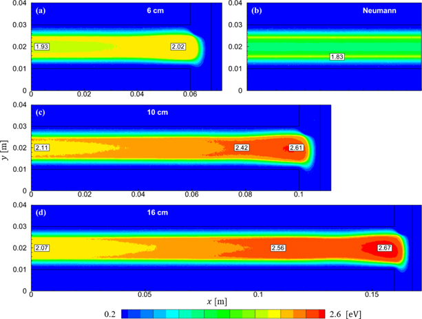
Figure 10. The time-averaged spatial profile of the effective electron temperature for (a) case 2, (b) case 1, (c) case 3, and (d) case 4.
Download figure:
Standard image High-resolution imageFigure 11 shows the time-averaged spatial profile of the direct ionization rate. In region A, figures 11(a), (c) and (d) show a similar pattern to that of figure 11(b), which has a uniform distribution. However, the ionization rate increases significantly in region C. The reaction rate in region B is much lower than in regions A and C, so it has a slightly faint distribution. Even though the electron temperature is high in region B, the number of electrons having higher energy than the ionization threshold energy is lower than in region C. Thus, the high electron temperature is used for the easy plasma transport, which results in a lower electron density. For this reason, the density in region B appears low, while the overall electron density increases in region C as the electrode length increases.
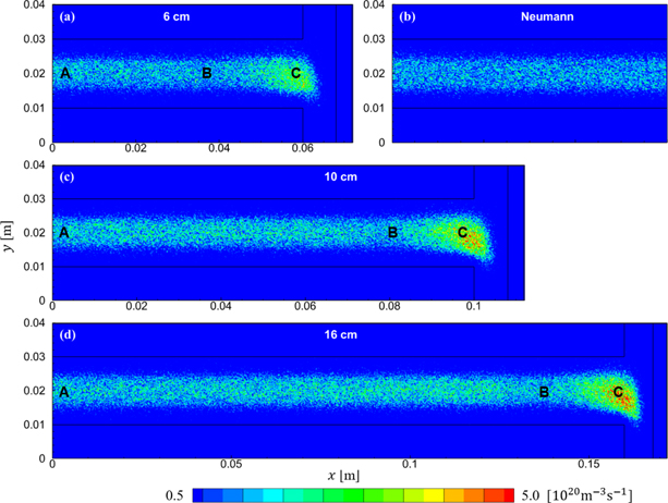
Figure 11. The time-averaged spatial profile of the direct ionization rate for (a) case 2, (b) case 1, (c) case 3, and (d) case 4.
Download figure:
Standard image High-resolution imageFigure 12 compares the 1D slices of the electron density and electron temperature in the y-direction in regions A and C. The electron density is lower in region A and much higher in region C than that in case 1. The electron density in region A is symmetrical in the y-direction, whereas the electron density in region C is slightly skewed toward the bottom electrode. The heated electrons at the edge of the bottom electrode participate in the ionization, and the ionization rate at the lower part of region C is high, as shown in figure 11. Compared to the 1D results (Neumann boundary condition case), the electron heating effect in the x-direction increases the electron temperature in the whole region because of the nonlocal kinetics. This tendency is enhanced as the electrode length increases. With electrode lengths of 6 and 16 cm, the electron temperature distribution in region A does not show a big difference between the two cases. In the bulk plasma of region C (0.015 < y < 0.025 m), the electron temperature profile in the 6 cm case is flat while that of the 16 cm case is convex upward. These differences are attributed to the strong electron heating in the x-direction near the sidewall and the electrode edge. In particular, as the electrode length increases, the large increase in the x-directional electron heating brings about the increase in the electron temperature in the bulk plasma (near y = 0.02 cm). In other words, the electrons smoothly move in the x-direction with the characteristics of nonlocal kinetics. Consequently, the electron temperature, ionization rate, and electron density increase.

Figure 12. The time-averaged y-directional spatial profiles of (a), (b) the electron (solid) and the ion (dashed) densities and (c), (d) the electron temperature (Te) at (a), (c) region A and (b), (d) region C.
Download figure:
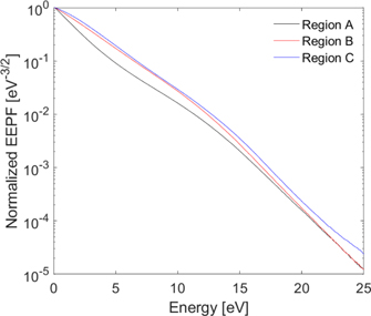
Standard image High-resolution imageFigure 13 shows the normalized electron energy probability function (EEPF) in the three regions: region A (x = 0.0), region B (x = 0.132 m), and region C (x = 0.156 m) for cases 4. The EEPF shows a bi-Maxwellian distribution in region A, but more like a Maxwellian in regions B and C. The energy relaxation mean free path of electrons in argon gas is 3 cm or longer at 100 mTorr for low-energy electrons (ε < 11.6 eV) [8], and thus electrons heated at the bulk-sheath boundary in region A are detected at the bulk center without energy loss. Thus, the electrons have a bi-Maxwellian distribution in region A. However, for the energetic electrons capable of inelastic collisions, the energy relaxation length (λε ) is shorter than the gap size of the system, and the EEPF is depleted again for ε > 11.6 eV. Because the transport length in the horizontal direction is longer than λε while being affected by electron heating in the x-direction, the electrons heated near the sidewall can transport horizontally, resulting in the high-temperature EEPF close to Maxwellian in regions B and C. In particular, the EEPF in region B is drawn similarly to region C for the low-energy electrons (ε < 11.6 eV) because the energy relaxation length is longer than the distance between region B and C. However, the EEPF follows the graph of region A for the high-energy electrons (ε > 16 eV) because the transported electrons with this high energy already made the ionization collisions in region C and lose their energy.
Figure 13. The EEPFs of cases 4 at regions A, B, and C.
Download figure:
Standard image High-resolution image
In fluid approximation, the electron transport coefficient is affected by the distribution function of the low-energy electrons with a high population. Thus, the electron transports in regions B and C are more prominent than that in region A. As to the ionization coefficient, however, the high energy tail is more important to exceed the threshold energy. Accordingly, the electron density in region C increases due to increased ionization reactions with the large population in the high energy tail. However, the electron density in region B decreases as the ionization is smaller than that in region C while the transport is still high. Comparing regions A and B, the ionization rates are almost the same for the high-energy electrons (ε > 16 eV), but the particle transport is much faster in region B than in region A because of the higher electron temperature. Therefore, the electron density in region B becomes even lower than that in region A. The distance from the sidewall to region B is related to the energy relaxation mean free path, which is controlled by the gas pressure.
4. Conclusions
The tendency of nonuniformity of the primary plasma parameters has been analyzed using a parallelized 2D PIC simulation with the increase of the electrode length. A GPU-based parallelization of a PIC simulation made it possible to calculate the particle dynamics of 2D CCPs accurately. In contrast to the 1D PIC simulations, where the axial (y-direction) sheath motion influences the discharge characteristics dominantly, it was found that the x-directional dependency cannot be neglected even for a long electrode. The results show that the edge effect significantly varies the density distribution and electron heating profiles. With the analysis of nonlocal electron kinetics from the phase-resolved potential, electron flux, and electron power deposition, we found out that the spatial inhomogeneity is attributed to not only the variation of ionization profiles caused by the nonuniform electric field but also the electron transport property depending on energy distributions. In addition, nonuniformity cannot be neglected even for a large aspect ratio of the electrode size to the gap distance because it is always triggered at the edge. As the ratio increases at a fixed applied voltage, the nonuniformity becomes larger. Even with a very large distance from the sidewall to the plasma, the asymmetric edge of the electrode also causes this nonuniformity. There could be other reasons affecting the plasma uniformity in CCPs, such as the standing wave effect, electronegativity and chemical reactions [34], and so on, but the nonlocal kinetic effect can be detected only with the PIC simulations. The investigation for the methods to reduce nonuniformity is the future work of this research.
Acknowledgments
This work was supported by the National Research Council of Science & Technology (NST) grant by the Korean government (MSIT) (No. CRC-20-01-NFRI) and by National R&D Program through the National Research Foundation of Korea (NRF) funded by the Ministry of Education, Science and Technology (Grant No. NRF-2019R1A2C1088518).
Data availability statement
The data that support the findings of this study are available upon reasonable request from the authors.