

Abstract
An electrosurgical argon plasma with a 5% admixture of molecular hydrogen is studied in order to investigate time averaged plasma parameters by optical emission spectroscopy (OES). Electron densities in the range of 1015–1016 cm−3 are determined from the Stark broadening of the time averaged line profiles of the Balmer-α and -β emission lines of hydrogen. A two-profile fit corresponding to regions of different electron densities is found to provide a better representation of the line broadening than a single profile fit. This is consistent with time resolved ICCD imaging, acquired with 150 ns time resolution, that shows strong radial gradients in the plasma emission and the asymmetry produced by the discharge arrangement. Gas temperatures are determined using two different methods. Firstly, simulated spectra for different rotational temperatures are fitted to the measured N2(C-B, 0-1) emission band originating from ambient air diffusion into the argon/hydrogen gas flow. From the best fit, rotational temperatures between 1500 K and 1800 K are inferred. These measurements are in good agreement with those inferred by the second method, which is based on the collisional broadening of the emission lines of neutral argon at 750 nm and 751 nm. This latter method may be useful for the measurement of gas temperatures when the device is used inside hollow organs during endoscopic or laparoscopic interventions, where air mixing will be limited. Therefore, the results of this study are highly relevant to applications of these devices, e.g. for controlling tissue effects and the avoidance of excessive heating.
Export citation and abstract BibTeX RIS
1. Introduction
Since the mid 20th century electrosurgery is frequently used during surgical interventions for applications such as precise cutting of tissue, resection of tumors, hemostasis and coagulation of bleeding wounds [1]. Instruments, which may be handheld, laparoscopic or endoscopic, are typically operated in either monopolar or bipolar modes. Monopolar techniques consist of instruments with one active pointed electrode powered by a high voltage radio frequency (RF) generator (a so-called electrosurgical unit or ESU) and a large passive patient return electrode. The alternating RF-voltage applied between the electrodes leads to a current flow through the patient and thermal heating of the tissue—up to temperatures of more than 100 °C—within several microseconds. This results in tissue desiccation and/or partial vaporisation. The large asymmetry between the electrodes means that the effect is very local due to the high current density in the vicinity to the active electrode. Bipolar instruments consist of an active and return electrode integrated into the same device and are both in contact with the treatment area. These devices, which are often designed in a scissors or clamp geometry enable faster severing of tissue or coagulation with reduced bleeding.
A commonly used monopolar method for superficial hemostasis, coagulation and ablation of tissue is argon plasma coagulation (APC) [2–5]. Here, the conductive channel between the active electrode and the surface of the patient develops in an argon gas flow, which is passed through the instrument to the treatment area. Due to a voltage of several kV a thin discharge channel of several millimetres in length is formed that induces tissue effects over an area of approximately 1 cm2 in timescales smaller than 1 s. This contactless plasma treatment prevents tissue sticking to the electrode, which can be an advantage over other electrosurgical coagulation techniques, and allows larger areas to be treated within short time periods by moving the device across the tissue.
The APC technique is well-established, so there is abundant information on the optimisation of tissue effects and their relation to the electrical control parameters of the discharge [3, 6]. Nonetheless, plasma conditions in surgical interventions might differ strongly between two applications. Since the device is operated by hand or endoscopically, a constant working distance cannot be easily achieved and can vary between 0 mm and more than 10 mm during a procedure. Moreover, the electrical characteristics of the tissue are changed during APC treatments. These changes have the potential to influence effects induced on the tissue due to possible changes in current densities. Such effects also impose limitations and difficulties for the in situ characterisation of the plasma. In general, there are a limited number of published studies aimed at characterisation of plasma parameters for this particular device [7, 8].
Due to the small size of the plasma volume and high electron density [7], invasive electrical probes, such as Langmuir probes (see e.g. [9]) are not applicable to determine plasma parameters in electrosurgical devices, as they would disturb the plasma and induce significant changes in the discharge characteristics. With regard to the clinical application of the APC non-invasive active spectroscopic methods, such as absorption spectroscopy or laser induced fluorescence, are not suited for an in situ characterisation for technical reasons. Therefore, only passive spectroscopic methods, such as optical emission spectroscopy (OES), are suitable for characterisation of plasma parameters, such as the gas temperature, electron density and electric field, in such devices as shown in [7].
In [7], electron densities and electric fields in an APC source were determined by an OES diagnostic method based on the combination of numerical simulations and the measurement of the absolute intensity of molecular nitrogen emission. For that particular method, the density of molecular nitrogen needs to be known, and therefore nitrogen was actively introduced into the discharge-forming gas mixture. The use of molecular nitrogen is motivated by the fact that its emission spectrum under elevated pressure conditions consists of two electronic systems: N2(C-B) ('second positive system') and  (B-X) ('first negative system') which show very different upper state energies, namely 11.05 eV and 18.74 eV. This large difference in energies means that the nitrogen emission spectrum is very sensitive to variations of the electron energy distribution function in nitrogen-containing plasmas. Therefore the combination of OES measurements and collisional-radiative (CR) models for nitrogen emission can be used to infer information about the electron energy distribution function and the electric field [10]. In addition, the lifetimes, rate constants for collisional quenching and cross sections for electron impact excitation of these molecular nitrogen states are comparatively well-known. Furthermore, this diagnostic method was successfully compared to other diagnostic methods, such as Langmuir probe [11], multipole-resonance-probe [12] and current–voltage measurements [8], at plasma conditions, where these methods are reliable.
An obvious disadvantage of the described method for plasma characterisation is that the density of molecular nitrogen needs to be known. Moreover, this density cannot be arbitrarily low, because of the limited sensitivity of the detectors used to measure the emission. As a result, well-defined conditions, such as those used in [7] are needed for the application of this nitrogen-based method. Since the APC device is frequently used in minimally invasive interventions, including internal treatments of hollow organs (stomach, bladder etc), the conditions required to apply the described nitrogen-based diagnostics may not always be fulfilled. Therefore, alternative non-invasive passive OES methods are required. One well-established option is the analysis of the spectral broadening of atomic emission lines for the determination of electron densities and gas temperatures [13–18].
The analysis presented in this work uses the profiles of argon and hydrogen atomic lines for the characterisation of an APC source. Since argon is used as working gas during the APC application and hydrogen is produced, in principle, by electron impact dissociation of water vapour formed during the interaction of the discharge with the treated tissue, emission lines of these two gases are naturally present in the measured spectra. Nevertheless, in this study an admixture of 5% hydrogen is used in order to increase the signal-to-noise ratio (SNR) of the hydrogen line emission. The Stark broadening of the Balmer lines, Hα and Hβ, is studied to determine the electron density (ne). These lines are frequently used for measurements of ne since their line shape is highly sensitive to the interaction with electrons and ions due to the linear Stark effect [13]. The same applies for Hγ , which could not be used in this work due to interfering emission lines and a lower SNR. Unlike hydrogen emission lines, argon lines are typically much less influenced by Stark broadening under the conditions studied here and their broadening is mainly driven by van der Waals and resonance effects. The evaluation of all three broadening mechanisms enables the determination of gas temperatures (Tg) in non-equilibrium atmospheric pressure plasmas, as demonstrated in the recent literature [16–21] for a variety of plasma sources.
Due to the transient behaviour and the physical asymmetry of the APC discharge arrangement, significant gradients of plasma parameters are assumed, especially in the axial direction between active electrode and the tissue. These gradients are reinforced due to ambient air diffusion and the evaporation of water from the tissue. To study these effects, spatio-temporal imaging is used to demonstrate the strong gradients in plasma emission. Furthermore, spatially and temporally averaged spectral measurements are performed over the whole discharge channel as well as regions of interest close to the electrode and close to the tissue and compared with previous studies [7, 8].
2. Emission spectrum analysis
Atomic and molecular transitions can both be used for the characterisation of APC plasma conditions. The emission spectrum of a plasma depends not only on the density of the excited species but also on the thermal movement of emitting particles, collisions with surrounding species and surrounding electromagnetic fields, among others [13, 24, 33]. These influences produces a certain shape of atomic emission lines as a result of a variety of broadening mechanisms which will be described in the following section.
2.1. Concept and definitions of spectral line broadening mechanisms
Atomic emission lines have a natural width ΔλN ∝ ΔE, where ΔE is the energy spread of the transition. ΔE is connected through the Heisenberg uncertainty principle to the finite lifetime Δt of the emitter due to spontaneous emission. This effect is called natural broadening. The width ΔλN is usually very small (in the order of 10−4 nm) and can be neglected in most experiments. The various interactions between the emitter and the plasma mentioned above translate into a reduction of the lifetime of the transition; and thus, in an increase of ΔE and the line width Δλ. These broadening mechanisms produce line profiles that are typically Lorentzian in shape. Furthermore, broadening effects due to the motion of the emitters produce an emission profile in the shape of a Gaussian. Both types of broadening mechanisms are well described in several articles and books [13–15, 22]. The measured line profile is a convolution of this Lorentzian part, L, and the Gaussian part, G, and can therefore be described as a Voigt function, V, defined as

where Te indicates the electron temperature in K and '*' a normalised convolution. If the contribution of individual broadening mechanisms to the measured profile is known, it is possible to determine fundamental plasma parameters from the overall line profile.
Any device that is used to measure the photoemission of a plasma, such as a spectrometer, shows a characteristic instrumental profile. This induces an instrumental broadening of the emission line profile, here represented by ΔλI, the full width at half maximum (FWHM). This profile can be measured in detail or approximated by a function, typically a Gaussian.
Doppler broadening is caused by a changing frequency (wavelength) of light due to the thermal motion of emitting particles. Assuming that the particle velocity distribution is given by a Maxwellian distribution, the Doppler width of the Gaussian Doppler profile is proportional to  and can be calculated as presented e.g. in Djurovic et al. [23].
The convolution of two Gaussian profiles results in another Gaussian profile [24]. Hence, assuming that the profile produced by the instrument is Gaussian in shape, the instrumental width can be combined with the Doppler width to give an overall Gaussian profile, whose width ΔλG is expressed as follows:

Pressure broadening is a collective term for resonance, van der Waals and Stark broadening. These mechanisms all result in a close to Lorentzian-shaped profile.
Resonance broadening is an effect caused by the interaction between two identical atoms that is confined to transitions involving a level that is dipole-coupled to the ground state. The FWHM attributed to resonance broadening as a function of  , ΔλR, is calculated as described in detail e.g. in [23, 25, 26].
Van der Waals broadening is the result of the dipole interaction of an excited atom (the emitter) and the induced dipole of a neutral perturbing atom in the ground state. The calculation of the FWHM of van der Waals broadening ΔλvdW can be derived as a function of  from [15, 17, 19, 23, 27].
Stark broadening is the result of the splitting and the shift of energy levels of a particle carrying an electric dipole moment, when subjected to an external electric field. This effect results in a shift and broadening of the fine structure components of the emitted transition as a consequence of the interaction with charged particles in the plasma and can be used to measure the electron density ne [24].
The overall width of the convolution of these individual Lorentz profiles, which is also Lorentzian in shape [24], can be calculated by

Taking ΔλL and ΔλG into account, the width of the overall Voigt profile ΔλV can be expressed as

If ΔλV is known the individual contribution of a certain broadening mechanism to the overall line width can be derived using equations (2)–(4).
2.2. Voigt fitting procedure
One possible option for the determination of plasma parameters (ne, Te, Tg) from a measured line profile is, to fit a synthetic Voigt profile to the data points by a least square algorithm. This smooth Voigt profile is discretised and adapted to the resolution of the spectrometer by integrating over wavelength regions that correspond to the pixel size. In this way the overall width of the Gaussian and the Lorentzian profile ΔλG and ΔλL can be inferred and subsequently used to obtain physical quantities as described in the following sections. Uncertainties in the quantities measured are obtained by varying the fit parameters in a range for which the residual in the line centre (= data point − fit curve) does not exceed the residual of the best fit by 20%. For all emission lines investigated the background is negligible.
2.3. Gaussian contribution to the profile
To reduce the degrees of freedom of the Voigt fit, the Gaussian contribution to the profile is determined in advance and taken as fixed input parameter. This follows from the work of Konjevic et al [15], where it was shown that using a fixed Gaussian decreases systematic errors in the determination of the Stark width while fitting with a Voigt function.
For all lines investigated here, the Gaussian contribution is dominated by the instrumental profile. Due to the variable resolution of the echelle spectrometer, the instrumental width needs to be measured close to the wavelength region of interest. This can be achieved, for example, by using the line emission of a low pressure plasma system. Here, a low pressure double coil inductively coupled plasma (ICP) operated in argon (500 W, 5 Pa) [29] is used. The instrumental widths related to the hydrogen Hα and Hβ transitions are determined from nearby argon emission lines (Ar I, λ = 470.2 nm and λ = 687.1 nm). Due to the relatively high mass of argon and Tg ⩽ 800 K measured in this low pressure system, other broadening mechanisms can be neglected for these lines. Therefore, ΔλI is equal to the FWHM of the Gaussian fit to these lines. In a similar procedure the instrumental line widths related to the argon lines used in this study are inferred.
For the Doppler broadening, the gas temperature Tg is needed. A useful and reliable method for the determination of a gas temperature under low and atmospheric pressure conditions is the analysis of the rotational structure of an excited diatomic molecule [30]. Spectral analysis is performed under the conditions, that the three translational and two rotational degrees of freedom of the molecule are in equilibrium. In that case, it can be assumed that Trot = Tg. At atmospheric pressure this equilibrium is typically achieved through frequent collisions between the excited state investigated and the background gas during the lifetime of the excited state. These collisions thermalise the rotational population distribution before photoemission [30].
In this work, the 'second positive system' (N2(C-B)) of nitrogen is used to infer the gas temperature. Under the conditions studied here, the excitation of nitrogen can be described by direct electron impact excitation, step-wise electron impact excitation via the metastable N2(A) state or by collisions with argon metastables. It has previously been discussed in [7, 31, 32] that, in atmospheric pressure plasma sources using argon as a background gas, excitation via argon metastables could increase the rotational temperature of N2(C-B) above the gas temperature, and therefore decrease the reliability of this method for the determination of Tg. However, in the APC source the fractional density of argon metastables should be relatively low due to quenching by air and water vapour entering the plasma region, in contrast to argon plasma sources operated in more controlled atmospheres. As a result, the influence of argon metastables on the rotational temperature should be limited. In addition, due to the high collision frequency of N2(C) with surrounding non-excited argon atoms, the translational and rotational degrees of freedom of N2(C) reach an equilibrium during its lifetime. Therefore, the rotational temperature measured from the N2(C-B) emission under considered plasma conditions should be equal to the gas temperature [32].
The measured vibrational bands of N2(C-B, 0-0) at λ ≈ 337 nm and N2(C-B, 1-0) at λ ≈ 316 nm which usually show the most intense emissions, and therefore, the best SNRs are overlapped by the emissions of OH(A-X, 0-0) at λ ≈ 306 nm and NH(A-X, 0-0) at λ ≈ 336 nm. Therefore, in this work only the rotational sequence of the N2(C-B, 0-1) vibrational band at λ ≈ 358 nm is used. Neighbouring vibrational bands (N2(C-B, 1–2, 2–3, ...)) show overlapping emission which would cause inaccuracies in the determination of Tg. Next to the vibrational bands of OH(A-X) and NH(A-X) mentioned above, intense emission from the CN(B-X) transition at λ ≈ 388 nm is observed in the APC emission spectra. The rotational structures of these diatomic molecules are not suitable for temperature determination, since their excitation mechanisms are not clear under the conditions studied here. For example, these radicals can possess additional rotational energy by dissociation of polyatomic molecules or by excitation by argon metastables, which could cause systematic errors in the gas temperature determination [33, 34].
To determine the gas temperature, the N2(C-B, 0-1) spectrum is simulated using the code described in [10] for different rotational temperature values and compared to the measurements. The code uses Hönl–London factors and rotational level populations to determine the emission intensity of the relevant transitions. By finding the best fit between measured and simulated spectra the gas temperature and confidence interval are determined. To simplify the fitting procedure N2(C-B) spectra for different rotational temperature values in steps of 20 K are calculated for the spectral resolution of the applied spectrometer. The actual fit is performed manually to avoid potential errors induced by overlapping emission of different atomic and molecular species with N2(C-B), which are either produced by excitation of the feed gas or evaporated tissue material.
Using Tg from the rotational band fitting, the Doppler widths ΔλD for hydrogen and argon lines are calculated. The overall Gaussian width for each line of interest ΔλG is calculated from ΔλI and ΔλD after equation (2).
2.4. Lorentzian contribution to the profile
The width of the Lorentzian contribution as a result of the fitting procedure is analysed in order to separate the impact of certain broadening mechanisms. This is described below for hydrogen and argon atomic emission lines.
2.4.1. Electron density determination from the line broadening of hydrogen lines
The electron density is determined from the Stark width  contributing to the overall Lorentzian profile of Hα or Hβ. Since the resonance broadening shows negligible impact for hydrogen lines [35], ΔλL in equation (3) can be simplified to:

where the van der Waals width ΔλvdW is calculated for atmospheric pressure using Tg derived from the N2(C-B) emission. Under given conditions excited states of nitrogen and hydrogen show comparable lifetimes, which are considerably shorter than the duration of an ignition pulse [36, 37]. Therefore, since both emissions are excited by electron impact, the gas temperature measured using N2(C-B) emission characterises temporally and spatially the same plasma conditions as during the excitation of atomic hydrogen emission.
Electron densities are determined from the Stark width using formulas from Gigosos et al. [14] including the effects of ion dynamics. For Hβ the density in cm−3 is inferred from the FWHM,  , with the following approximate formula, which is independent of Te:

For Hα the 'full width half area' (FWHA)  , which is much less influenced by the ion dynamics, is used instead of the FWHM:
The calculation of  is described in detail in [14]. For this purpose,
  is determined in advance and a synthetic Lorentzian Stark profile is produced. From this profile
  is inferred by integration. Approximate formulas, such as (6) and (7) are described in [15] to have a typical uncertainty of 5%–12%, not including the uncertainty in the fitted Stark width, which amounts to approximately 10%–15%.
Stark broadening of Hβ and Hα depends weakly on the electron temperature. Equations (6) and (7), that include ion dynamics were inferred to filter out the explicit dependence on Te. However, using the tables from Gigosos et al. [14], the dependence can be recovered and it is possible to estimate Te by plotting pairs of ne and Te that are consistent with the measured values of ΔλS(Hβ) and ΔλS(Hα). This procedure yields two curves, where the crossing point (within the experimental uncertainties) indicates an estimate of the values of ne and Te simultaneously, as described by Torres et al. [38]. The use of the tables presented in [14] requires the knowledge of the temperature ratio of the electrons and ions, expressed by the reduced mass parameter μ. Since this is not known in advance, a range of 5 ⩽ μ ⩽ 10 is chosen. The electron density obtained using this approach shows good agreement with those inferred from equations (6) and (7) and a Te of approximately 15 000 K ± 40%, which is close to the value measured in [7] under similar conditions. The large uncertainty of 40% is not only a product of the used range for μ but also of the uncertainty in the measurements of ΔλS and the weak dependency on Te indicated above.
2.4.2. Gas temperature determination from the line broadening of argon lines
Another method to determine the gas temperature is the use of line broadening methods [16–19, 21]. Theoretically, Doppler, resonance and van der Waals broadening show a dependence on Tg. Rodero et al. [18] presented a method to determine Tg by using van der Waals and resonance broadening of atomic argon lines corresponding to transitions into the resonance levels s2 and s4 of the 3p54s configuration.
The sum of resonance and van der Waals broadening widths, which is from here on referred to as the collisional broadening width, ΔλC, is given by the width of the Lorentzian profile, excluding the Stark width for argon atomic lines  :
:

For argon,  shows a linear dependence on the electron density, which is given as

Here ne is given in cm−3 and wS indicates the Stark parameter in nm, that is reported by several authors for a large number of argon lines under various plasma conditions [13, 39]. To determine the Lorentzian width, which is needed to calculate ΔλC, Voigt profiles are fitted to the measured Ar I line profiles.
The gas temperature can be found graphically by plotting theoretical values of ΔλC as a function of Tg. For known ne, the collisional width ΔλC is obtained from equation (8) using wS (see table 1) and the corresponding Tg can be inferred directly from the curve. In principle, 14 Ar lines from the transitions into the s2 and s4 states of the 3p54s configuration can be used. Only some of those lines are observed, due to gaps in the measured spectra due to the spectral sensitivity profile of the spectrometer. Other lines show a very low intensity, hence only two lines are used in this work, namely at λ = 750.39 nm and λ = 751.46 nm. For these lines, further referred to as Ar I-750 nm and Ar I-751 nm, the collisional broadening is calculated similar to [17, 19, 27] using the following equation

for a feed gas mixture of Ar:H2, with χAr and  the molar fractions of Ar and H2.
Table 1. Van der Waals and resonance broadening constants (in nm K0.7 and nm K) for Ar–Ar and Ar–H2 emitter–perturber configurations [18]. The Stark parameter wS in nm is given for Te = 10 000 K [39].
| Line | CvdW,Ar |

| CR,Ar | wS |
|---|---|---|---|---|
| Ar I-750 nm | 1.89 | 2.85 | 53.78 | 0.0085 |
| Ar I-751 nm | 1.71 | 2.57 | 13.37 | 0.0074 |
Constants CvdW (in nm K0.7) and CR (in nm K) for van der Waals and resonance broadening for Ar are taken from [18] and are calculated for H2 as presented in [18]. The dipole polarisability  for H2 is found in [40]. The values used are given in table 1.
2.5. Single fit vs double fit
A single Voigt profile fit, which leads to a single electron density or gas temperature for the whole plasma volume is most suited for uniform plasmas. In this study, the plasma is assumed to have electron density gradients due to the complexity of the physical system and the temporal evolution of the discharge. Therefore, fitting is also performed using a combination of two Voigt profiles, as proposed in [41]:
where ne,i and Tg,i represent the two different electron densities and gas temperatures and η is the intensity ratio of the two single profiles. The double Voigt fit is performed in the first step by fitting the outer line wings only with a single profile V1, where the contribution of the second profile V2 can be neglected. The resulting width, ΔλL,V1, is taken as input parameter for the two profile fit. Then the width of V2, ΔλL,V2, and the intensity ratio η is determined by a least square algorithm.
3. Experimental setup and measurement procedure
3.1. Experimental setup
The experimental setup is shown schematically in figure 1. It consists of a RF-power generator (VIO 3, Erbe Elektromedizin GmbH) connected to an APC 3 module (Erbe Elektromedizin GmbH). A polyethylene hose encloses the pointed active electrode of the endoscopic instrument used (FiAPC 2200a probe, ø = 2.3 mm, l = 2.2 m). The tip of the APC probe is mounted vertically above the tissue surface at an adjustable distance. A passive return electrode is realised as a stainless steel plate that functions as a sample holder. To ignite a plasma, a high voltage pulse of up to 5 kV is applied between the two electrodes. This voltage pulse is applied as a damped sinusoidal waveform with a frequency of 350 kHz and is modulated at 20 kHz (see figure 2). To lower the breakdown voltage and to confine the ignition zone, a laminar feed gas flow is fed through the probe to the treatment area. For flow control an external mass flow controller (Bronkhorst High-Tech, FG-201CV-AGD-33-E-DA-A1V) is used to ensure a constant gas flow of 1 slm. In contrast to pure argon, which is usually used for this electrosurgical device, here an admixture of 5% H2 is added to the argon feed gas, to increase the emission intensity of hydrogen lines. To monitor the stability of the plasma, current–voltage waveforms are measured with a differential voltage divider (TESTEC, TT-SI 9010, dividing factor of 1:1000) and a Rogowski probe (Pearson model 6585, 1.0 V per A). Traces recorded using an oscilloscope (LeCroy WaveRunner 204MXi-A, 2 GHz) are shown in figure 2.

Figure 1. Experimental setup to perform optical measurements. The ESA 4000 (LLA Instruments GmbH & Co. KG, Germany) broadband echelle spectrometer and the ICCD camera are triggered on the beginning of the plasma ignition via current trigger. Current and voltage traces are recorded with an oscilloscope.
Download figure:
Standard image High-resolution image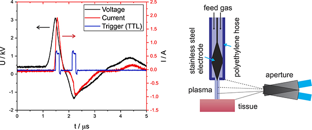
Figure 2. (Left) Current and voltage traces during the discharge. The normalised TTL trigger pulses are used to synchronise the ICCD camera measurements to different phases of the discharge. (Right) Schematic of the APC probe and the fibre position for the spatially resolved OES.
Download figure:
Standard image High-resolution imageRaw pork neck slices are used as tissue samples as they are readily available and reproducible. A stainless steel autopsy blade is used to prepare the samples into slices of constant thickness. Slices of 4 mm × 5 cm × 3 cm are vacuum-packed in plastic foil and stored at −18 °C. The samples are thawed in a water bath of 25 °C for 1 h in order to bring them to ambient temperature before measurements are carried out.
3.2. Spectral measurements
For spectroscopic diagnostics of the plasma, a calibrated broad-band echelle spectrometer (ESA 4000, LLA Instruments GmbH & Co. KG, Germany) with a resolution of ΔλI = 15 pm at λ = 200 nm and ΔλI = 60 pm at λ = 870 nm [28] is used. This resolution is high enough to resolve the rotational structure of vibrational molecular bands and the broadening of atomic emission lines. However, the spectrometer has a complex spectral efficiency structure including several regions of zero sensitivity above 500 nm, which prevents the observation of some of the argon lines in the infrared. The construction of the spectrometer and the calibration procedure are described in [10].
Measurements of the emission spectra of the APC discharge are synchronised to the discharge current with a pulse delay generator (Stanford Research Systems, Model DG353). Each spectrum consists of the time integrated emission of 500 ignition pulses, during an exposure time of 25 ms. 36 single spectra are averaged for statistical purposes, which also provides a better SNR. Non-spatially resolved measurements are performed with an open fibre end. Since the surface of the sample is not perfectly flat, the fibre is aimed at an angle of 15° to ensure the proper collection of the emitted light. As the water content and degree of carbonisation of the tissue changes during the measurement, the position of the APC instrument above the tissue is changed after every spectrum measured. The distance between the end of the nozzle and the tissue in this case is kept constant at 2 mm.
3.3. Spatially resolved measurements
Since the spectral measurements introduced in the last section show neither spatial nor temporal resolution, measurements with a four channel ICCD camera (hsfc pro, PCO) are performed to get information about the spatio-temporal dependency of the plasma emission. Two-dimensional images (integrated over the line of sight) of the plasma emission in the spectral range from 300 nm to 1000 nm are acquired at different times during the current pulse for a probe–tissue distance of 2 mm. The spatial resolution of the images is equal to 120 pixels per millimetre. The camera operates with an integrated pathway of beam splitters and four identical ICCD chips. As a result, it is possible to take up to eight pictures (double shutter mode) within the same current pulse. In this way four pictures are taken during the first positive phase and four during the first negative phase of the current waveform. Two of these eight measurement windows of 150 ns are shown in figure 2 as rectangular signals (maximum and minimum of the alternating current). Since both images originate from the same channel, and are only analysed qualitatively, no sensitivity calibration is necessary.
In order to correlate the information from the ICCD camera images to local plasma parameters, spatially resolved OES is carried out using the echelle spectrometer and optical fibre at two different regions in the discharge channel, namely: near the electrode and near the tissue surface, as shown in figure 2 (right). An aperture of 5 cm length with an opening diameter of 1 mm is used to confine the viewing angle, which is measured with a point-like light source and a goniometer. The full diameter of the acceptance cone of the spectrometer at the position of the APC plasma channel amounts to about 1.5 mm. To better differentiate between spatial effects in the two plasma regions, the probe–tissue distance is increased to 4 mm for these measurements, compared to 2 mm for all other measurements.
4. Results and discussion
4.1. Gas temperatures from N2(C-B) rotational bands
A sample N2(C-B) spectrum, measured from the whole discharge channel and a probe–tissue distance of 2 mm, is shown in figure 3 (left). By manually fitting the normalised simulated spectrum to the measured N2(C-B,0-1) emission band for different rotational temperatures Trot, the gas temperature is obtained from the best fit. Overlapping lines from argon ions (Ar II) are excluded from consideration (see figure 3 (left)). The theoretical accuracy of gas temperature measurements depends on the statistical variation of the measured intensity with respect to the background. Under the conditions studied here, the theoretical confidence interval induced by the manual fitting amounts to about ± 60 K. Nevertheless, the analysis of multiple repeated measurements leads to an uncertainty of approximately ± 200 K. Possible reasons for this large variation are differences in nitrogen impurities in the discharge channel and variations in the roughness and composition of the top layer of the treated sample. During APC treatments the condition of the top layer of the tissue change rapidly as a result of desiccation, coagulation and carbonisation, which has an influence on the plasma conditions, dissipated power and gas temperature. Moreover, partial vaporisation of tissue material by the large electric current of the spark channel causes water vapour to be mixed into the working gas mixture, and additional collisional quenching of excited nitrogen molecules.
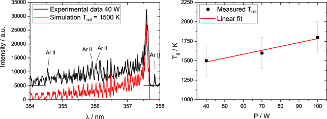
Figure 3. (Left) Example experimental and simulated spectra of the N2(C-B, 0-1) rotational emission band used for the gas temperature determination for a probe–tissue distance of 2 mm. The measured spectrum is shifted vertically for clarity. (Right) Measured gas temperatures as function of the output power of the VIO 3 generator.
Download figure:
Standard image High-resolution imageThe inferred temperatures are shown in figure 3 (right) as a function of the generator power P. Values for P indicate the maximum output power set at the electrosurgical unit, which can differ from the power absorbed by the plasma by up to 10%. It is observed, that the temperature rises slightly from approximately 1500 K to approximately 1800 K when the output power is increased from 40 W to 100 W, which is in good agreement with previous studies on this plasma source [7].
4.2. Electron density determination with Hβ and Hα
The values for Tg determined above enable the Doppler width of Hβ and Hα to be inferred. Measured instrumental widths are shown in table 2 and can be used to obtain the total Gaussian width ΔλG of these lines from equation (2). Further, knowledge of Tg allows the van der Waals width ΔλvdW of the lines to be inferred (see table 3).
Table 2. Measured and calculated Gaussian contributions in nm to the experimental line width of Hβ and Hα for the corresponding gas temperatures shown in figure 3. Uncertainties are approximately 10%.
| Line | P (W) | ΔλI | ΔλD | ΔλG |
|---|---|---|---|---|
| Hβ | 40 | 0.033 | 0.014 | 0.036 |
| 70 | 0.014 | 0.036 | ||
| 100 | 0.015 | 0.036 | ||
| Hα | 40 | 0.039 | 0.018 | 0.043 |
| 70 | 0.019 | 0.044 | ||
| 100 | 0.020 | 0.044 |
Table 3. Inferred van der Waals and Stark widths ΔλS and ΔλSA in nm for Hβ and Hα (single fit—index 's'). Lorentzian and Voigt widths are calculated by equations (4) and (5) using values from table 2.
| Line | P(W) | ΔλvdW | ΔλS,s | ΔλSA,s | ΔλL,s | ΔλV,s |
|---|---|---|---|---|---|---|
| Hβ | 40 | 0.034 | 0.71 | — | 0.74 | 0.75 |
| 70 | 0.032 | 0.77 | — | 0.80 | 0.80 | |
| 100 | 0.030 | 0.81 | — | 0.84 | 0.84 | |
| Hα | 40 | 0.037 | — | 0.16 | 0.19 | 0.20 |
| 70 | 0.036 | — | 0.16 | 0.20 | 0.20 | |
| 100 | 0.033 | — | 0.17 | 0.20 | 0.21 |
As an example, the resulting fit and residual using a single Voigt profile for Hβ are displayed in figure 4 (left) for P = 70 W. It is observed, that the single fit underestimates the emission intensity at the line centre (negative residual) and overestimates it just outside the line centre (positive residual). Only further to the wings is the emission intensity accurately represented. The three relevant parts of the line profile are demonstrated by the horizontal red line in the residual plot in figure 4 (left) for the left wing of the emission line.
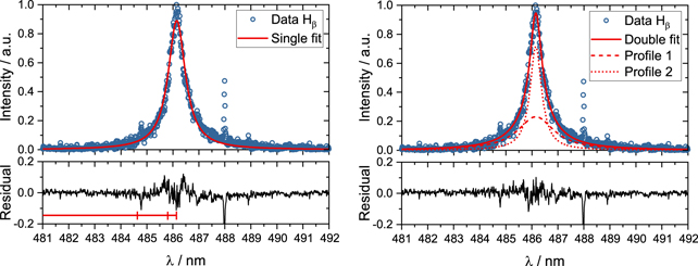
Figure 4. Single (left) and double (right) Voigt profile fits for Hβ at 70 W and a probe–tissue distance of 2 mm. The assumption of two electron densities in the plasma due to spatial gradients results in a better fit of the experimental data.
Download figure:
Standard image High-resolution imageThis preliminary fit indicates an electron density that is at least one order of magnitude higher than the lower limit (ne > 1014 cm−3) where fine structure effects have to be taken into consideration (see e.g. [22]). Due to the missing central component of the fine structure of Hβ, the line profile usually shows a dip in the centre that depends on the electron density and the homogeneity of the plasma. In spite of this fact the use of a Voigt profile for the approximation of data points for Hβ is a common procedure, as discussed by Konjević et al. [15]. However, for ne > 1015 cm−3, relatively low electron temperatures, and a fixed Gaussian width, a Voigt profile provides a reliable estimation of the Stark contribution to this line. Therefore, Voigt profiles will be used for both Hβ and Hα in the rest of the analysis. With the Lorentzian widths electron densities are obtained from equations (6) and (7) [15] considering the contribution due to van der Waals broadening (see table 3). The uncertainty of ΔλvdW is inferred from the uncertainty of Tg and amounts to approximately 10%.
Inferred Stark widths (FWHM and FWHA), ΔλL and the width of the Voigt profile ΔλV are listed in table 3. Under the conditions studied here, the influence of the van der Waals broadening is only relevant for Hα, as illustrated in figure 5, where the relative contributions of different broadening mechanisms for Hβ and Hα as a function of ne are shown. Here, the red dashed line represents an upper threshold calculation of the impact of ΔλvdW on the total Lorentzian width for Tg = 1500 K, which is the lowest value measured for Tg and therefore gives the largest value for ΔλvdW. The Stark width ΔλS is shown for comparison for Te = 15 000 K, as derived from the crossing point method discussed earlier. A small sensitivity to the Doppler broadening is found for both lines by applying equation (4) for a range of gas temperatures between 0 K and 3000 K. Since the contribution of the Doppler width ΔλD to the overall Gaussian width ΔλG is approximately 10%, as demonstrated by the values in table 2 and equation (2), the variation of ΔλD produces an uncertainty of approximately 1% in the value of ΔλV, which is negligible in comparison to the uncertainty of the Voigt fit (see section 2.4.1). This supports the use of a fixed Doppler width in the fitting algorithm. From this analysis, it can be concluded that ΔλL(Hβ) ≈ ΔλS and therefore the Lorentzian width of Hβ can be used directly for the determination of the electron density for ne > 1015 cm−3, whereas ΔλL(Hα) needs to be corrected for the van der Waals broadening.
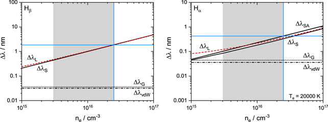
Figure 5. Stark widths  and
and  of Hβ and Hα [15] are shown as solid black lines. Additionally, ΔλG ≈ ΔλI and ΔλvdW for Tg = 1500 K are plotted to show the contribution of these broadening mechanisms to the total line width. The overall Lorentzian width is shown as a red dashed line. The range of observed densities in this work is shown as grey shaded area.
Download figure:
Standard image High-resolution imageElectron densities determined from the single fit are displayed in figure 6 (left) for generator powers of 40 W, 70 W and 100 W. The electron density as a function of the power is found to be almost constant and only slightly increases from 6 × 1015 cm−3 to 7.5 × 1015 cm−3. Similar values are found between Hβ and Hα. Furthermore, the electron densities measured here are in good agreement with those measured in [7, 8] under similar conditions. In these previous studies temporally and spatially averaged ne measurements were performed for the whole discharge channel using current density measurements and absolute measurements of the N2(C-B, 0-0) emission band by using Ar:N2 (95:5) as feed gas.
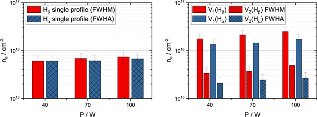
Figure 6. Electron densities ne for the single (left) and double (right) Voigt profile fitting procedure as a function of power P and a working distance of 2 mm after equations (6) and (7). Densities measured using the single profile are between those obtained from the two profile fit. Error bars include the uncertainty in the measurement of  and
and  and the uncertainty in the approximate formulas (6) and (7).
Download figure:
Standard image High-resolution imageIn figure 4 (right) the Hβ emission line is fitted using a double Voigt profile, where two Voigt profiles of different widths, corresponding to different electron densities, are combined. Here, V1 is used to refer to the broader of the two profiles corresponding to a higher electron density and V2 is used to refer to the narrower of the two, corresponding to a lower electron density. These double fits show an improved approximation of the measured line profiles which can be seen in the residual of the fit (see figure 4, right).
For this two profile fit, the correction of Hα for the van der Waals broadening is even more relevant (see figure 5) due to the lower electron density contribution. Two electron densities in the range of ne = 2.5 × 1016 cm−3 and ne = 3 × 1015 cm−3 for V1 and V2 are determined from each line as described above. Figure 6 (right) shows the electron densities obtained as a function of the generator power P. Again a similar trend with rising power is found for Hβ and Hα. Nevertheless, it should be noted that the small increases in electron density with increasing power are within the uncertainties of the measurements. This is consistent with the observations in [33] and may be explained by an increasing plasma diameter which would allow for a relatively constant current density and electron density in the plasma even as the overall current and power input is increased. For the double fit it is also found that densities inferred from Hβ are slightly higher than those from Hα. A reason for this could be the missing central component in the fine structure of Hβ, leading to a broader FWHM of the fitted Voigt profile.
The improved fits using the combination of two Voigt profiles indicates the presence of time averaged spatial gradients of the plasma electron density. In order to investigate this further, spatially resolved measurements are performed.
4.3. Spatially resolved measurements
Figure 7 shows the spectra for two different spatial locations (electrode region and tissue region) obtained by using an aperture (see figure 2 (right)). For these measurements the probe–tissue distance is set to 4 mm (compared to 2 mm for the previous sections) and the generator power to P = 70 W (see section 3.3). For clarity, three parts of the spectrum (indicated by the grey areas) are shown separately to mark some of the main differences between the two regions of interest. Atomic iron lines Fe I and Fe II (below 300 nm) originate only at the electrode. Hydrogen and argon lines from the feed gas are present in both electrode and tissue surface regions. The evaporation of tissue material leads to a modification of the gas composition in the plasma channel and induces changes in the measured emission spectra. Dissociation of water and biomolecules in the plasma cause the excitation of OH(A-X) (λ ≈ 280–325 nm), as found in e.g. [42, 43]) and CN(B-X) emission bands (λ ≈ 380–388 nm).

Figure 7. Emission spectra measured at two plasma regions, using the setup shown in figure 2 (right): (red) measured near the electrode, (black) measured near the tissue surface. Zoomed in views of three different parts of the spectra indicated by the grey boxes are shown to highlight important differences. In these zoomed in views, line profiles of Hβ are normalised to the areas, profiles of the argon lines are normalised to the maximum of Ar I-751 nm for better comparison.
Download figure:
Standard image High-resolution imageTo compare the details of the line profiles, the Hβ emission lines for both regions of interest are presented normalised to the same area in figure 7 (bottom, middle). This comparison reveals a broader line profile from the electrode region (red line), which indicates a higher average ne that decreases towards the tissue surface, where a more narrow profile is found (black line).
Possible reasons for this effect can be found in the measured ICCD camera images of the discharge. Figure 8 shows the plasma emission for a 2 mm working distance during two different phases of the alternating current pulse. The first picture (left) is taken during the maximum of the positive phase of the current waveform, while the second picture (middle) shows the plasma emission during the maximum of the negative phase. Both measurement windows are indicated in figure 2. Since the time integrated emission of one pulse is dominated by the emission of these two phases, they show a good representation of the temporal behaviour of the discharge. The measured plasma intensity is integrated along the horizontal axis for both cases and plotted in figure 8 (right). The emission profile during the positive phase (positive voltage applied to the electrode) suggests a spark discharge [10, 44, 45], which has a region of high intensity close to the positive electrode. Here, a higher electric field can be assumed due to the asymmetry of the two electrodes. For distances d ⩾ 0.6 mm from the powered electrode, the intensity is almost constant but a branching of the discharge channel is observed close to the tissue surface, leading to a low electron density contribution. During the negative phase (negative voltage applied to the electrode) an emission profile comparable to a glow discharge is observed. Moving from the electrode towards the tissue, this is characterised by areas of varying light emission, from a cathode dark space-like low emission close to the electrode (small yellow spot), to a region of high electron density and photoemission (negative glow, intensity maximum) followed by a much lower electron density in the positive column [45, 46]. This results in a lower emission intensity in the region for d ⩾ 1 mm. Additionally, the intensity of the positive column is much lower than that observed in the positive current phase. This might indicate a higher electron density for the spark discharge than for the glow discharge for d ⩾ 1 mm. The measured optical emission spectra however are time integrated. Therefore, since the exposure time of the spectrometer covers several 100 current pulses, both plasma states contribute to the measured signal. Images taken after the current maxima show a much lower intensity and therefore only a small contribution to the overall emission intensity.

Figure 8. ICCD camera images of the discharge at different phases of the current pulse. The pictures were taken at the maximum of the positive (left) and negative (middle) current half wave. The intensity (right) is integrated along the horizontal axis and plotted as function of the axial position. The APC probe and the tissue are redrawn in grey, since they are not visible in the original picture. The tip of the active electrode is shown schematically.
Download figure:
Standard image High-resolution imageMeasured electron densities obtained from the double Voigt fitting procedure for the two different regions of interest can be found in table 4. The narrow components V2 in both measurements show equivalent values for ne (within the uncertainty of the measurement), which is consistent with an outer radial region of lower electron density that is approximately uniform along the axis. A similar discussion can be found in [41, 47]. On the other hand, the contribution V1—consistent with an inner region with high electron density—shows values for ne near the electrode almost twice as high as the measurement close to the tissue surface. Figure 8 also shows a higher intensity near the electrode in both positive and negative current phases, while at the tissue surface most of the intensity is reduced to the positive current phase. Assuming that the population of the excited states of hydrogen is dominated by electron impact excitation, the observed intensities are consistent with the variation in ne as discussed above.
Table 4. Electron densities from spatially resolved measurements for an output power of P = 70 W and a probe–tissue distance of 4 mm. Uncertainties amount to ±30%.
| Location | ne(V1) (cm−3) | ne(V2) (cm−3) |
|---|---|---|
| Electrode | 1.9 × 10¹⁶ | 3.7 × 10¹⁵ |
| Tissue | 1.1 × 10¹⁶ | 4.0 × 10¹⁵ |
Therefore, the electron density variations within the discharge channel are the result of the general spatial asymmetry of the electrode system and the temporal behaviour of the discharge, which leads to differences in the density gradients in axial direction between electrode and tissue as a function of time. Additionally, radial gradients due to the cylindrical shape of the plasma occur in both positive and negative current phases. Close to the tissue other mechanisms, such as diffusion of water vapour or ambient air, might have an additional influence on the electron density due to the formation of negative ions.
The argon lines also change in intensity and shape depending on the spatial region observed (see figure 7 bottom right). The lines emitted from the tissue surface region have a symmetric profile, while those originating from the electrode show a small asymmetry on the red wing (right side of the emission profile). This indicates, that these line profiles consist of an intense Voigt profile, similar to the shape emitted near the tissue, and a second less intense contribution, that has a small wavelength shift to longer wavelengths and is emitted near the electrode only. The origin of this second line profile is not known in detail. One possible explanation could be a small spot at the tip of the electrode with high electron density and gas temperature, as discussed in [41]. From the shift of this profile with regard to the theoretical wavelength of the line an electron density of ne ≈ 1.5 × 1017 cm−3 ± 30% is measured, using the quadratic Stark shifts presented in [48]. This value for ne is consistent for both argon lines (Ar I-750 nm and Ar I-751 nm). The extra shift (evaluated at half intensity) produced by the inherent asymmetry caused by the quasistatic quadratic ion contribution [17, 23, 24, 50] amounts to about 4 pm for ne = 1017 cm−3 (inferred from equation (9.57) in [24] and equation (4) in [50], including impact and quasistatic broadening) which is approximately 3% of the total width of the line, is not considered in the estimate above. The fact that the high electron density contribution of the spot is not detected in the hydrogen profiles is likely to be a result of the combined effect of the small spot size, which leads to proportionally much weaker emission than the rest of the discharge, and the broad emission which merges with the background. Another possibility is the formation of excited dimers, also called excimers ( , see e.g. [31]). Emission transitions between attractive and repulsive excimer states can form wings from one or another side of natural argon atomic lines (e.g. transitions into the 3p54s states) [49, 51], which here show on the right side of the lines. Since they are effectively collisionally quenched by air and other molecules, this hypothesis would also be consistent with the absence of the asymmetry of Ar I-750 nm and Ar I-751 nm close to the tissue. Also the possible formation of wings due to an asymmetric instrumental profile (coma aberration of the applied spectrometer), as it is found e.g. in [52, 53] is taken into account. In principle, this could add another contribution to the line profile. However, the pronounced asymmetry in the measured argon lines is here considered to be unlikely produced by this effect since negligible asymmetries are found in the wings of the line emission from the low pressure plasma reference source [29] (see figure 9) and it is not present in the lines produced at the tissue region (see figure 7 bottom right).
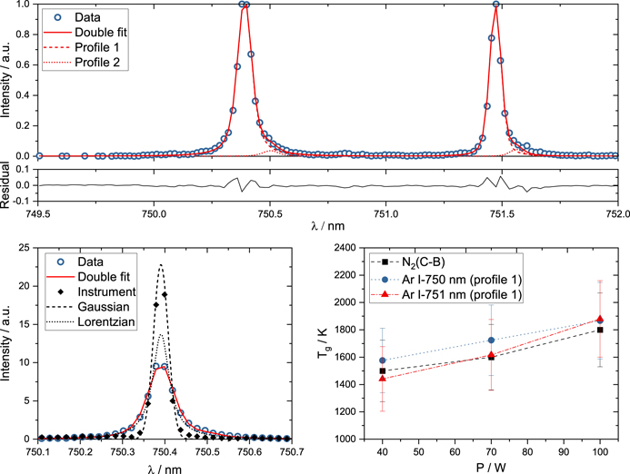
Figure 9. Double fit of Ar I-750 nm and Ar I-751 nm for 70 W (top). The fit is performed by using known parameters of ΔλG and ΔλS to determine the width of ΔλC. The Gaussian and Lorentzian components of the more intense profile 1 as well as the measured instrumental profile are shown bottom left for Ar I-750 nm (normalised to the same area). Measured Tg compared to those obtained from the simulation of N2(C-B) are shown bottom right.
Download figure:
Standard image High-resolution imageAnother difference between electrode and tissue emission are the N2(C-B) emission bands as presented in figure 7 (bottom left). Since these are originating from ambient air diffusion, they are not present in the electrode spectrum, as the strong gas flow ensures that air diffusion only becomes important at larger distances from the gas outlet. Therefore, the measured gas temperatures in section 4.1 are only valid for the tissue region. The presence of nitrogen molecular bands cannot be guaranteed in surgical interventions, such as interventions in hollow organs, due to different gas atmospheres and an increasing amount of feed gas. Therefore, using argon emission lines for gas temperature determination would be a powerful tool for the application of APC in the absence of nitrogen.
4.4. Gas temperature measurements by spectral line broadening of Ar I lines
Figure 9 (top) shows the Voigt fitting of the argon lines Ar I-750 nm and Ar I-751 nm for a generator power of 70 W. Since the measured argon lines show an asymmetric shape, two profiles are again used during the fitting procedure, as discussed in section 4.3. Only the more intense profile 1 is used for gas temperature determination. Due to the low intensity of profile 2, the FWHM of profile 1 is not changed. In figure 9 (bottom left) the Gaussian and Lorentzian components of the discretised Voigt profile are plotted in black. The Lorentzian emphasises the impact of the collisional broadening of these lines, indicated by the width ΔλC. Additionally, the measured instrumental profile from the low pressure discharge [29] is plotted. In this representation all profiles are normalised to the same area. Due to the relatively high mass of argon, the Doppler width of the argon emission lines is small in comparison to the instrumental width (ΔλI ≈ 14 ⋅ ΔλD). Therefore, ΔλD can be neglected for both argon lines and it is assumed that ΔλG = ΔλI = 41 pm. In table 5 the parameters used for both fits and the resulting width ΔλC are listed.
Table 5. Measured and calculated contributions to the experimental line width of Ar I-750 and Ar I-751. Due to the small Doppler width it is assumed that ΔλI = ΔλG. Listed values for ΔλC correspond to profile 1.
| Line | P (W) | ΔλG (nm) | ΔλS (nm) | ΔλC (nm) |
|---|---|---|---|---|
| Ar I-750 nm | 40 | 0.041 | 0.006 | 0.044 |
| 70 | 0.007 | 0.040 | ||
| 100 | 0.008 | 0.037 | ||
| Ar I-751 nm | 40 | 0.041 | 0.006 | 0.020 |
| 70 | 0.006 | 0.018 | ||
| 100 | 0.007 | 0.016 |
Since the argon lines show similar intensities in both spatial views (see figure 7), averaged electron densities from the single fit of Hβ are used to calculate the Stark widths  from equation (9). Thus, ΔλC can be inferred and used for Tg determination. It should be noted, that listed values for wS correspond to an electron temperature of Te = 10 000 K. However,
  is small in comparison to ΔλC, as can be seen in table 5, which moreover explains why these lines are also not sensitive to gradients in ne.
Measured temperatures from profile 1 (see figure 9 (top)) as a function of the power are shown in figure 9 (bottom right). Errors of Tg are determined from the uncertainty of ΔλC which is about 10%. The measured temperatures from Ar I-750 nm and Ar I-751 nm are consistent to each other. Additionally, they show the same trend and reproduce the gas temperatures obtained by the simulation of the N2(C-B, 0-1) emission band.
The van der Waals and resonance broadening constants that are required to determine the gas temperature from ΔλC via equation (10) are dependent on the gas phase collision partners and therefore the gas mixture. Since the gas mixture at a given spatial region is determined by mixing with ambient air and evaporation of water into the plasma, it is important to test whether the limited knowledge of the gas mixture affects the accuracy of the gas temperature measurements. Figure 10 shows the gas temperature as a function of ΔλC for both Ar lines and a series of different gas mixtures.

Figure 10. Dependency of ΔλC from the gas temperature for Ar I-750 nm and Ar I-751 nm for different gas mixtures. It is observed, that for higher temperatures (>2500 K) Tg is highly sensitive to smaller changes in ΔλC.
Download figure:
Standard image High-resolution image
Since the van der Waals broadening constants  (Ar I-750 nm) and
  (Ar I-751 nm) for water vapour are close to CvdW,Ar = 1.893 (Ar I-750 nm) and CvdW,Ar = 1.706 (Ar I-751 nm), ΔλvdW does not change significantly with the gas phase water content.
  was calculated by using values for the polarisability from [40]. Regarding equation (10), changes in ΔλC are mainly due to a decrease in ΔλR induced by a possible depletion of argon atoms in the plasma. This effect is most pronounced for lines with high CR,Ar, such as Ar I-750 nm. For the values of CvdW,air the reader is referred to [18].
Table 6 demonstrates the influence of different gas atmospheres on the gas temperature (see figure 10). It can be seen, that the absence of H2 (pure Ar) does not change the gas temperature significantly. Stronger influences are observed by the addition of 20% water vapour, where slightly lower values for Tg are found for both lines. For an addition of 20% air, Tg is decreased for Ar I-750 nm and increased for Ar I-751 nm. This contrasting behaviour is due to the small CR,Ar for Ar I-751 nm and the fact that CvdW,air is about a factor of 3 larger than CvdW,Ar. Since measured values for Tg using Ar:H2 do not show a significant deviation from the inferred values using the N2(C-B) molecular band, the fraction of water vapour and air is assumed to be smaller than 20%.
Table 6. Gas temperatures for different gas mixtures shown in figure 10 inferred from equation (10) for P = 70 W.
| Line | Ar (K) | Ar:H2 (K) | Ar:H2:H2O (K) | Ar:H2:air (K) |
|---|---|---|---|---|
| Ar I-750 nm | 1780 | 1730 | 1450 | 1620 |
| Ar I-751 nm | 1630 | 1620 | 1510 | 1880 |
From figure 10 a sensitivity range of the method for both lines used can be defined. In the case of Ar I-750 nm, this range is given between 0.02 nm ⩽ ΔλC ⩽ 0.08 nm and in the case of Ar I-751 nm between 0.01 nm ⩽ ΔλC ⩽ 0.06 nm. If ΔλC exceeds this range, changes in ΔλC do not affect Tg significantly. On the other hand, a ΔλC below these values would lead to large uncertainties. The measured width of ΔλC for the conditions used in this work are all found within the range of high sensitivity.
Due to the small Stark broadening  of these lines, it is possible to obtain the gas temperature, even if the electron density is not known precisely. The assumption of 1015 cm−3 ⩽ ne ⩽ 1016 cm−3 translates into a gas temperature that differs from the measured Tg
by ⩽ ± 15% for Ar I-750 nm, which is more dominated by van der Waals and resonance broadening than Ar I-751 nm. This deviation is within the error bar of the measurement (see figure 9).
of these lines, it is possible to obtain the gas temperature, even if the electron density is not known precisely. The assumption of 1015 cm−3 ⩽ ne ⩽ 1016 cm−3 translates into a gas temperature that differs from the measured Tg
by ⩽ ± 15% for Ar I-750 nm, which is more dominated by van der Waals and resonance broadening than Ar I-751 nm. This deviation is within the error bar of the measurement (see figure 9).
Glossary of symbols
5. Conclusion
In this work, various OES methods for the characterisation of an electrosurgical argon plasma were demonstrated.
Stark broadening of hydrogen lines was used to determine electron densities using an admixture of 5% H2 to the feed gas. A double Voigt fit was applied to take into account the spatio-temporal evolution of the plasma and good agreement was found between Hβ and Hα for this procedure. This agreement is beneficial for clinical applications, where no hydrogen is admixed to the feed gas and typically only Hα can be observed reliably from the dissociation of water. It should be noted, that in this clinical scenario the measured densities are only likely to be valid for the diffusion area of water vapour close to the tissue.
An alternative method to the well-established gas temperature determination by the simulation of N2 emission bands for different rotational temperatures has been tested. This method uses the broadening of Ar I lines, corresponding to transitions into the s2 and s4 resonance levels of the 3p54s configuration. Measured temperatures demonstrate a good agreement between both methods. Moreover, the gas temperatures determined from the two lines Ar I-750 nm and Ar I-751 nm used in this work were consistent with each other. It has been shown, that also in the presence of various perturbing gases, such as water vapour or air, Tg can be inferred using corrections to the collisional widths of the argon atomic lines. Even if the gas composition is not known precisely the assumption of pure argon does not lead to large deviations from the gas temperatures inferred by molecular bands of N2 near the tissue surface.
In conclusion, the use of the broadening of argon atomic lines may be a useful alternative for measurements of the gas temperatures below 2500 K in scenarios, where no nitrogen is present. This is the case in hollow organs during endoscopic interventions. Since the Stark broadening of these lines is small, this method allows in principle to estimate the gas temperature with an error of ⩽ ± 15% even if only the order of magnitude of the electron density is known. Both OES diagnostic methods used in this study provide similar results under conditions where both methods are applicable and when combined offer the possibility of plasma characterisation over a wide range of conditions.
Table 7. Symbols used in this study indicating the line width due to different broadening mechanisms.
| Symbol | Explanation |
|---|---|
| λ | Wavelength of the optical transition |
| ΔλN | Natural line width |
| ΔλG | Overall Gaussian width (Doppler and instrumental width) |
| ΔλD | Doppler broadening width |
| ΔλI | Instrumental profile width |
| ΔλL | Overall Lorentzian width (van der Waals, resonance and |
| Stark width) | |
| ΔλvdW | Van der Waals broadening width |
| ΔλR | Resonance broadening width |

| Stark broadening width for hydrogen atomic lines |
| (FWHM) | |

| Stark broadening width for hydrogen atomic lines |
| (FWHM) | |

| Stark broadening width for argon atomic lines (FWHM) |
| ΔλC | Collisional broadening width (van der Waals and resonance |
| broadening) |
Acknowledgements
This work was funded by the German Federal Ministry of Education and Research (BMBF) in the frame of the project `IDA' (13N14341) and supported by the German Research Foundation (DFG) with the Collaborative Research Center CRC1316 `Transient atmospheric plasmas: from plasmas to liquids to solids' (project B5). The authors acknowledge Professor Kurt Behringer and Dr. Sven Gröger for their valuable inputs on spectral line broadening.