
Abstract
In this review we describe a transient type of gas discharge which is commonly called a streamer discharge, as well as a few related phenomena in pulsed discharges. Streamers are propagating ionization fronts with self-organized field enhancement at their tips that can appear in atmospheric air, or more generally in gases over distances larger than order 1 cm times N0/N, where N is gas density and N0 is gas density under ambient conditions. Streamers are the precursors of other discharges like sparks and lightning, but they also occur in for example corona reactors or plasma jets which are used for a variety of plasma chemical purposes. When enough space is available, streamers can also form at much lower pressures, like in the case of sprite discharges high up in the atmosphere. We explain the structure and basic underlying physics of streamer discharges, and how they scale with gas density. We discuss the chemistry and applications of streamers, and describe their two main stages in detail: inception and propagation. We also look at some other topics, like interaction with flow and heat, related pulsed discharges, and electron runaway and high energy radiation. Finally, we discuss streamer simulations and diagnostics in quite some detail. This review is written with two purposes in mind: first, we describe recent results on the physics of streamer discharges, with a focus on the work performed in our groups. We also describe recent developments in diagnostics and simulations of streamers. Second, we provide background information on the above-mentioned aspects of streamers. This review can therefore be used as a tutorial by researchers starting to work in the field of streamer physics.
Export citation and abstract BibTeX RIS

Original content from this work may be used under the terms of the Creative Commons Attribution 4.0 licence. Any further distribution of this work must maintain attribution to the author(s) and the title of the work, journal citation and DOI.
1. Introduction
Streamers are fast-moving ionization fronts that can form complex tree-like structures or other shapes, depending on conditions, see e.g. figure 1. In this paper, we review our present understanding of streamer discharges. We start from the basic physical mechanisms and concepts, aiming also at beginners in the field. We also touch on related phenomena such as discharge inception, diffuse discharges, nanosecond pulsed discharges, plasma jets, transient luminous events and lightning propagation, electron runaway and high energy radiation.

Figure 1. A 3 μs long exposure, false color, image of a peculiar streamer discharge caused by a complex voltage pulse. Image taken from [1].
Download figure:
Standard image High-resolution imageThe paper is organized as follows: in the present introductory section we briefly review streamer phenomena in nature and technology, we discuss the relevant physical mechanisms with their multiscale nature and we have a first look at numerical models and streamers in laboratory experiments. The following two sections are devoted to the details of the different temporal stages of the discharge evolution: discharge inception in section 2 and streamer propagation and branching in section 3. In these two sections we mainly concentrate on streamers in ambient air but in section 4 we treat streamers in other media and pressures. In section 5 this is followed by discussions on streamer-relevant plasma theory and chemistry, interaction with flow and heat, high energy phenomena, plasma jets and sprite discharges. The final main sections treat the available methods in detail, first modeling and simulations in section 6, and then plasma diagnostics in section 7. We end with a short outlook and an overview of open questions on the physics of streamer discharge phenomena in section 8.
1.1. Streamer phenomena in nature and technology
The most common and well-known occurrence of streamers is as the precursor of sparks where they create the first ionized path for the later heat-dominated spark discharge. Streamers play a similar role in the inception and in the propagation of lightning leaders. Streamers are directly visible in our atmosphere as so-called sprites, discharges far above active thunderstorms; they will be discussed in more detail in section 5.6.
Streamers are members of the cold atmospheric plasma (CAP) discharge family. Most industrial applications of streamers and other CAPs (i.e., not as precursors of discharges like sparks) utilize the unique chemical properties of such discharges. The highly non-equilibrium character and the resulting high electron energies enable CAPs to start high-temperature chemical reactions close to room temperature. This leads to two major advantages compared to thermal plasmas and other hot reactors: firstly it enables such reactions in environments that cannot withstand high temperatures, and secondly it can make the chemistry very efficient as no energy is lost on gas heating.
A key property of streamers is that the electric field at their tips is strongly enhanced. Electrons in these high-field regions can have typical energies of the order of 10 eV or higher. Such electrons can trigger chemical reactions that are out of reach for thermal processes, as 1 eV corresponds to a temperature of 11 600 K. In air and air-like gas mixtures this leads to the production of OH, O and N radicals as well as of excited species and ions like  , O−, O+,
  and
and  after an initial production of
  ,
,  , see section 5.2. Each of these species can start other chemical reactions, either within the bulk gas, on nearby surfaces or even in nearby liquids when the species survives long enough and can be easily absorbed. The initial distribution of the generated excited species is typically far from thermal equilibrium.
Due to these properties of streamers and other CAPs they are used or developed for a myriad of applications, most of which are described extensively in the following review papers [2–5]. Popular applications are plasma medicine [6–8] including cancer therapy [9] and sterilization [10], industrial surface treatment [11], air treatment for cleaning or ozone production [12, 13], plasma assisted combustion [14, 15] and propulsion [16, 17] and liquid treatment [18, 19]. Two recent reviews on nanosecond pulsed streamer generation, physics and applications are by Huiskamp [20] and Wang and Namihira [21].
A fast pulsed discharge like a streamer has the advantage that the electric field is not limited by the breakdown field. The electric field and thereby the electron energy can transiently reach much higher values than in static discharges. Pulsed discharges can be seen as energy conversion processes, as sketched in figure 2. First, pulsed electric power is applied to gas around atmospheric pressure. When the gas discharge starts to develop, this energy is converted to ionization and to free electrons with energies in the eV range, far from thermal equilibrium. The further plasma evolution can include different physical and chemical mechanisms. (a) Electric breakdown means that the conductivity increases further by ionization, heating and thermal gas expansion; it is used in high voltage switchgear, and has to be controlled in lightning protection. (b) Excitation, ionization and dissociation of molecules by electron impact trigger plasmachemical reactions in the gas, see section 5.2. (c) The drift of unbalanced charged particles through the gas can create so-called corona wind, see section 5.3. (d) If the local electric field is high enough, electrons can keep accelerating up to electron runaway, and create Bremsstrahlung photons in collisions with gas molecules; the photons can initiate other high-energy processes in the gas, as is in particular seen in thunderstorms, see section 5.4.

Figure 2. Energy conversion in pulsed atmospheric discharges with application fields.
Download figure:
Standard image High-resolution imageStreamer discharges are often produced in ambient air. For this reason, we and many other authors use the term standard temperature and pressure (STP) as a simple definition of ambient conditions. Their exact definitions vary, but they always represent a temperature of either room temperature or 0 °C (STP) and a pressure close to 1 atm. Here, we mostly refer to technological or laboratory discharges and therefore prefer the NIST definition of STP, which is also called normal temperature and pressure and is defined as 20 °C and 101.325 kPa [22].
1.2. A first view on the theory of streamers
In this section we will discuss the basics of streamer discharges. The theory is here explained for streamers in atmospheric air, but the concepts are also valid for or can be generalized to other gas densities and/or compositions.
Streamer discharges can appear when a gas with low to vanishing electric conductivity is suddenly exposed to a high electric field. Key for streamer discharges are the acceleration of electrons in the local electric field and the collisions between electrons and neutral gas molecules. For brevity, we will use the term gas molecules instead of writing gas atoms or molecules. The electron-molecule collisions can be of the following type:
- Elastic collisions, in which the total kinetic energy is conserved, although some of it is typically transferred from the electron to the gas molecule.
- Excitations, in which some of the electron's kinetic energy is used to excite the molecule. Depending on the gas molecule, there can be rotational, vibrational and electronic excitations.
- Ionization, in which the gas molecule is ionized.
- Attachment, in which the electron attaches to the gas molecule, forming a negative ion.
Data for the collisions of electrons with different types of atoms and molecules can be found, e.g., on the community webpage www.lxcat.net.
In a gas that is activated by earlier discharges, by external radiation or by radioactivity, free electrons to start the discharge can be provided by mechanisms such as detachment from negative ions or Penning ionization.
As explained below, streamer discharges can form where the electric field is high enough to support a continuous growth of the electron density. However, due to local field enhancement, streamers can also enter into regions where the electric field previously was too low. Field enhancement is the nonlinear streamer mechanism, which is based on the following physical processes.
1.2.1. Impact ionization
Free electrons that are accelerated by a high local electric field, can create new electron-ion pairs when they impact with sufficient kinetic energy on gas molecules. If there is also an electron attachment reaction, then the impact ionization rate must be larger than the attachment rate for the plasma to grow; the local electric field is then said to be above the breakdown value. In such fields, the chain reaction of exponential ionization growth leads to the creation of electrically conducting plasma regions.
How many ionization and attachment events occur per electron per unit length is described by the ionization and attachment coefficients α and η. Breakdown requires that α > η, or in other words, that the effective ionization coefficient

is positive. The electric field Ek
where the effective ionization coefficient vanishes  , is called the classical breakdown field; for E > Ek
, the ionization density grows exponentially with a characteristic length scale
, is called the classical breakdown field; for E > Ek
, the ionization density grows exponentially with a characteristic length scale  .
.
In electronegative gases like air, electron loss due to recombination with positive ions is negligible relative to attachment, because recombination is quadratic in the degree of ionization, and the degree of ionization is small.
In electropositive gases like pure nitrogen, there is no attachment and the breakdown field vanishes, but a substantial electric field is required nevertheless for efficient ionization avalanches. Similarly, there can be a balance between electron attachment and detachment reactions, e.g., in the upper atmosphere, which leads to an effectively vanishing attachment rate, as it is termed in the gas discharge literature. In the lightning literature, this situation is sometimes called a breakdown below the breakdown field.
1.2.2. Electron drift
Electrons gain kinetic energy in the local field and lose energy in collisions with gas molecules. This leads to an average drift motion that can be described by vdrift = −μe E, where μe is the electron mobility. Only in very high fields, electrons can overcome the friction barrier caused by collisions; they then keep accelerating and become runaway electrons. For further discussion see section 5.4.
The drift motion of charged particles in the field leads to an electric current that usually satisfies Ohm's law

where j is the electric current density and σ the conductivity of the plasma. Note that magnetic fields are not taken into account here, as their effect is typically negligible, see section 5.1.
As long as electron and ion densities are similar (i.e., during and after the ionization process and before attachment depletes the electrons), the electron contribution dominates the conductivity, hence σ ≈ eμe ne, where e is the elementary charge and ne the electron density. Ions also drift in the field, but as they carry the same electric charge and are much heavier, they are much slower than the electrons. Furthermore, ions lose kinetic energy more easily than electrons as they have a similar mass as the gas molecules they collide with; this is a consequence of the conservation of energy and momentum in collisions.
1.2.3. Electric field enhancement
Equation (2) shows that in an ionized medium with conductivity σ, an electric field E creates an electric current density j. Due to the conservation of electric charge

the charge density distribution ρ changes in time due to a current density j, and the electric field E changes as well according to Gauss' law of electrostatics in vacuum or in not too dense gases,

where  0 is the dielectric constant.
Equations (2)–(4) imply that the interior of a body with fixed shape and with constant conductivity σ is screened on the time scale of the dielectric relaxation time

while a surface charge builds up at the outer boundary of the body, that screens the field in the interior. If the shape of the conducting body is elongated in the direction of the electric field, there is significant surface charge around the sharp tips, and therefore a strong field enhancement ahead of these tips. If the locally enhanced field at a tip exceeds the breakdown value Ek , a conducting streamer body can grow at such a location, even if the background field is below breakdown. This is illustrated with numerical modeling results in figure 3.

Figure 3. Simulation example showing a cross section of a positive streamer propagating downwards. The range used for each linear color table is indicated on top, except for the light emission which is here given in arbitrary units. A strong electric field is present at the streamer tip. A charge layer surrounds the streamer channel, with both positive charge (blue, saturated) and negative charge (red) present. A cross section of the instantaneous light emission is also shown, which is concentrated near the streamer head. The simulation was performed with an axisymmetric fluid model [23] in air at 1 bar, in a gap of 1.6 cm with an applied voltage of 32 kV.
Download figure:
Standard image High-resolution imageTo be more precise, there are two important corrections to this simple picture of field screening in streamers. First, the shape of the conducting streamer body changes in time, and therefore the electric field is typically not completely screened from the interior. Second, the ionization and hence the conductivity of a streamer is not constant, but changes in space and time; for a generalization of the dielectric relaxation time to a reactive plasma with  , we refer to [24].
1.2.4. Electron source ahead of the ionization front
The above mechanisms suffice to explain the propagation of negative (i.e., anode-directed) streamers in the direction of electron drift. However, positive (i.e., cathode-directed) streamers frequently move with similar velocity against the electron drift direction. They require an electron source ahead of the ionization front. The dominant mechanism in air is photo-ionization, a nonlocal mechanism. Photons are generated in the active impact ionization region at the streamer tip, but create electron-ion pairs at some characteristic distance determined by the photon absorption length. Other sources of free electrons ahead of a streamer ionization front can be earlier discharges, radiation sources like radioactive elements or cosmic rays, electron detachment from negative ions, or bremsstrahlung photons from runaway electrons.
1.2.5. Coherent structures
The nonlinear interaction of impact ionization, electron drift and field enhancement creates the streamer head, as shown in figure 3. While in linear problems the sum of two solutions is a solution as well, the nonlinear interaction of forces can establish so-called 'coherent structures'. One of the first examples of a coherent structure is the soliton, a water wave in a straight channel that approaches a steadily propagating shape; it forgets about its initial conditions and approaches a uniformly translating profile, called the attractor of the nonlinear dynamics. Planar streamer ionization fronts without photoionization have been shown to be coherent structures [25, 26], similar to chemical or combustion fronts.
The full streamer head with its curved space charge layer seems to be a coherent structure as well, which has been demonstrated in a particular 2D Cartesian simulation [27], but beyond this case, it is currently just a common observation in simulations. For an earlier review of the nonlinear dynamics of streamers from the point of view of pattern formation, we refer to [28]. Considering the streamer head as a coherent structure opens up the pathway to reduce models of multi-streamer processes to tree models [29], as sketched in figure 4(d) and discussed further in section 6.4.

Figure 4. The multiple spatial scales in streamer discharges: (a) collision of an electron with an atom or molecule, (b) multiple electrons accelerate in a local electric field, collide with neutral gas molecules and form an ionization avalanche, (c) a branching streamer discharge with field enhancement at the tips, (d) a discharge tree with multiple streamer branches. Panel (d) is reproduced from a figure in [29].
Download figure:
Standard image High-resolution image1.3. The multiple scales in space, time and energy
The multiple spatial scales in a streamer discharge are illustrated in figure 4. From small to large, the following processes take place:
Collisions: On the most microscopic level [panel (a)], electrons that are accelerated by the electric field collide with gas molecules. A proper characterization of the collision processes is key to understanding the electron energy distribution as well as the excitation, ionization and dissociation of molecules.
Motion of an ensemble of electrons: Panel (b) in figure 4 shows an ensemble of 'individual' electrons moving in an electric field, colliding with gas molecules, and forming an ionization avalanche. The modeling of such electrons with Monte Carlo particle methods is described in sections 1.4.1 and 6.1.
Field enhancement and streamer mechanism: Panel (c) in figure 4 illustrates a streamer discharge with local field enhancement at the channel tips, as described above. The picture shows the result of a 3D simulation [23]. Such simulations are often performed with fluid models, which use a density approximation for electrons and ions, see sections 1.4.2 and 6.2.
Multi-streamer structures: In most natural and technical processes, streamers do not come alone, and they interact through their space charges and their internal electric currents. A reduced model that approximates the growing streamer channels as growing conductors with capacitance is shown in panel (d) of figure 4 and discussed in more detail in section 6.4; such so-called fractal models are a key to understanding processes with hundreds or more streamers.
Different scales in time and energy: A pulsed discharge starts from single electrons and avalanches, and eventually it develops space charge effects and a thin discharge layer around the ionized body to form a streamer. Later, behind the streamer ionization front, the ion motion, the deposited heat and consecutive gas expansion, and the initiated plasma-chemistry become important. These mechanisms can cause a transition to a discharge with a higher gas temperature and a higher degree of ionization. Such discharges are known as leaders, sparks and arcs.
All these scales and physical mechanisms depend on the temperature and pressure of the gas, and also on the gas composition, as will be discussed in later sections. The exception is the electron energy at the streamer head; its scale in the eV range is set by the ionization energy of the relevant molecules or atoms. However, electron runaway in sufficiently high electric fields can accelerate electrons into the range of tens of MeV in the streamer-leader phase of lightning, in a not yet fully understood process, as will be discussed briefly in section 5.4.
In sections 2, 3 and 5.3, we will discuss the temporal sequence of physical processes in a pulsed discharge in detail.
1.4. Introduction to numerical models
We now briefly introduce two types of models that are often used to simulate streamer discharges: fluid and particle models. A more detailed description of these models and their range of validity can be found in section 6.
1.4.1. Particle description of a discharge
Microscopically, the physics of a streamer discharge is determined by the dynamics of particles: electrons, ions, neutral gas molecules and photons. The electrons and ions interact electrostatically through the collectively generated electric field. Their momentum p and energy ɛ change in time as

where q is the particle's charge and v its velocity. The energy and momentum gained from the field is however quickly lost in collisions with neutral gas molecules. As the typical degree of ionization in streamers at up to 1 bar is below 10−4 (see sections 3.4 and 4.2), charged particles predominantly collide with neutrals rather than with other charged particles. In a particle-in-cell (PIC) code for streamer discharges, it is therefore common to describe the electrons as particles that move and collide with neutrals, the slower ions as densities, and the neutrals as a background density. To reduce computational costs, each simulation particle typically represents multiple physical electrons.
In a PIC code, the electron and ion densities are used to compute the charge density ρ on a numerical mesh. The electric potential ϕ and the electric field E = −∇ϕ can then be computed by solving Poisson's equation

with suitable boundary conditions, where ɛ is the dielectric permittivity. Note that the electrostatic approximation is used here; its validity is discussed in section 5.1. For more details about particle models and their advantages and disadvantages compared to fluid models, see section 6.1.
1.4.2. Fluid models
Fluid models employ a continuum description of a discharge, which means that they describe the evolution of one or more densities in time. In the classic drift-diffusion-reaction model, the electron density ne evolves as

where De is the electron diffusion coefficient and Sph is a source term accounting for nonlocal photo-ionization. The source term Se corresponds to electron impact ionization α and attachment η, and is usually given by

where E = |E|. Depending on the gas composition, one or more ion species can be generated. In the simplest case, these ions are assumed to be immobile and ion conversion processes are not followed in the model. A single density ni that describes the sum of positive minus negative ion densities can then be used, which changes in time as

Due to the conservation of electric charge, the source terms have to be equal in equations (7) and (9).
The transport coefficients μe and De and the source term Se in equation (7) depend on the electron velocity distribution. They are often parameterized using the local electric field or the local mean energy, see section 6.2. Details about the computation of photo-ionization are given in section 6.7. An example of a simulation of a positive streamer discharge in atmospheric air with the classic fluid model is shown in figure 3.
It should be noted that the reactions in the classical discharge model only contain interactions of discharge products like electrons, ions or photons with neutrals, and not directly with each other, except through the electric field. The reason is that the degree of ionization in a streamer at up to atmospheric pressure is typically below 10−4. Processes that are quadratic or higher in the degree of ionization are therefore negligible. This is discussed in more detail in section 4.2.
1.5. A first view on streamers in experiments
We have started with models, because they allow understanding how microscopic mechanisms interact to create the inner nonlinear structure of a single streamer. The challenge for modeling lies in covering multi-streamer processes and discharge phenomena on longer time scales based on proper micro-physics input. This will be treated in later sections.
For experiments, the situation is quite the opposite: it is easier to observe phenomena with many streamers over longer times than to zoom into the inner structure of single streamer tips on the intrinsic nanosecond time scale. Therefore, all streamer experimental images shown here are of complete discharges containing one or more streamer channels.
The easiest to acquire, and therefore the most often shown quantity in streamer experiments is the light emission. Light can easily be imaged by ICCD or other cameras. See sections 7.2 and 4.1 for limitations of this diagnostic. In air, a camera will only image the actively growing regions of a streamer discharge, i.e., the tips, while the current carrying channels mostly stay dark, as the electric fields and hence the electron energies are too low in the channels to excite the molecules to emissions in the optical range. This effect is demonstrated in figure 5 where for short exposures only small dots are visible.

Figure 5. Example of ICCD images for positive streamer discharges under the same conditions using different gate (exposure) times, as indicated on the images. The camera delay has been varied so that the streamers are roughly in the center of the image. The discharges were captured in artificial air at 200 mbar with a voltage pulse of about 24.5 kV. Image from [30].
Download figure:
Standard image High-resolution imageFigure 6 shows long exposure images of streamers in different gases and pressures. It showcases the wide variety of shapes and sizes of streamers, ranging from single channels to complex streamer trees at higher pressures. It also shows the variability in streamer width and branching behavior between the different conditions.

Figure 6. Overview of positive streamer discharges produced in three different gas mixtures (rows), at 1000, 200 and 25 mbar (columns). All measurements have exposure times between 2 and 6 μs and therefore show the entire discharge development, including transition to glow for 25 mbar. Image adapted from [31].
Download figure:
Standard image High-resolution imageTwo examples of the development of a streamer discharge at an applied voltage of 1 MV over a distance of 1 m in ambient air can be seen in figure 7. The top panel shows positive streamers propagating smoothly from the top (HV) electrode to the grounded bottom electrode. These streamers are, in the end, met by short negative counter-propagating streamers and then they develop into a hot, spark-like channel. The bottom panel shows that negative streamer expansion from the top electrode instead happens in bursts, likely related to the microsecond voltage rise time, see section 3.5. Almost simultaneously, positive streamers are growing from the elevated bottom electrode. These meet each other after around 550 ns, again forming a spark-like channel.

Figure 7. Development of positive (top panel) and negative (bottom panel) streamers creating a high-voltage spark in gap lengths of 100 and 127 cm respectively at applied voltages of 1.0 and 1.1 MV respectively, both with a voltage rise time of 1.2 μs in atmospheric air. Each picture shows a different discharge under the same conditions with increasing exposure time from discharge inception. In the top panel these times are (for (a)–(j)): 70, 160, 190, 250, 320, 340, 370, 410, 460 and 610 ns. In the bottom panel they are indicated on the images. Images from [32, 33].
Download figure:
Standard image High-resolution image2. The initial stage: discharge inception
The formation of a discharge requires two conditions: first, a sufficiently high electric field should be present in a sufficiently large region. Second, free electrons should be present in this region. If no or few of these electrons are present, the discharge may form with a significant delay or not at all. On the other hand, a sufficient supply of free electrons can reduce the inception delay and jitter, and also the required electric field to start a discharge within a given time.
Below, we will first discuss possible sources of free electrons, and then the conditions on the electric field to start a discharge, both in the bulk and near a surface. Finally, we discuss inception clouds, a stage immediately before streamer emergence near a pointed electrode in air.
2.1. Sources of free electrons
In repetitive discharges, one discharge can serve as an electron source for the next discharge. Depending on the time span between them, some electrons can still be present, or they can detach from negative ions like  or O− in air, or they can be liberated through Penning ionization. Another possibility is storage on solid surfaces.
For the first discharge in a non-ionized gas, possible electron sources are the decay of radioactive elements within the gas or external radiation. The actual mechanisms depend on local circumstances. E.g., in the lab, the materials used for the vessel and the lab itself, together with possible radioactive gas admixtures, determine the local radiation level. UV light can supply electrons as well, especially from surfaces which can emit for much lower photon energies than gases.
In the Earth's atmosphere, the availability of free electrons strongly depends on altitude; we discuss it here in descending order. Above about 85 km at night time or about 40 km at day time, the D and the E layer of the ionosphere contain free electrons. In fact, the lower edge of the E layer at night time can sharpen under the action of electric fields from active thunderstorms, and launch sprite discharges downward which are upscaled versions of streamers at very low air densities [34–36], see also section 5.6. On the other hand, electrons are scarce at lower altitudes, as they easily attach to oxygen molecules. In particular, in wet air, water clusters grow around these ions and electron detachment is very unlikely [37]. On the other hand, when a high energy cosmic particle enters our atmosphere, it can liberate large electron numbers in extensive air showers which could be a mechanism for lightning inception [38]. Up to 3 km altitude, the radioactive decay of radon emitted from the ground is the main source of free electrons [39], except for specific local soil conditions.
2.2. Avalanche-to-streamer transition far from boundaries
2.2.1. Starting with a single free electron
The simplest case to consider is a single free electron in a gas in a homogeneous field. According to equations (7) and (8), the ionization avalanche grows if the effective Townsend ionization coefficient  in a given electric field strength E is positive, i.e., if E > Ek
. During a time t, the center of an avalanche drifts a distance d = μe
Et in the electric field, and the number of electrons is multiplied by a factor
in a given electric field strength E is positive, i.e., if E > Ek
. During a time t, the center of an avalanche drifts a distance d = μe
Et in the electric field, and the number of electrons is multiplied by a factor  .
.
Eventually, the space charge density of the avalanche creates an electric field comparable to the external field. At this moment, space charge effects have to be included, and the discharge transitions into the streamer phase. In ambient air, this happens when  ; this is known as the Meek criterion. The avalanche to streamer transition is analyzed in [40]. In particular, it was found that electron diffusion yields a small correction to the Meek number, and that it determines the width of avalanches. In contrast, Raizer [41] relates the width of avalanches to electrostatic repulsion which is not consistent with the concept that their space charge is negligible.
When a single electron develops an avalanche in an inhomogeneous electric field E(r), the local multiplication rates  add up over the electron trajectory L like
  . The Meek criterion for the avalanche to streamer transition in air at STP is then

The Meek number gets a logarithmic correction in the gas number density when it deviates from atmospheric conditions [40]. This follows from the scaling laws discussed in section 4.2.
If there are Ne electrons starting together from about the same location, the required electron multiplication for an avalanche to streamer transition decreases with log Ne, since the criterion becomes ![${N}_{\text{e}}\enspace \mathrm{exp}\left[{\int }_{L}\overline{\alpha }\left(E\left(s\right)\right)\enspace \mathrm{d}s\right]\approx \mathrm{exp}\left(18\right)$](https://content.cld.iop.org/journals/0963-0252/29/10/103001/revision3/psstabaa05ieqn15.gif) .
.
2.2.2. Starting with many free or detachable electrons
When the initial condition is a wide spatial distribution of electrons in an electric field above breakdown, streamer formation competes with a more homogeneous breakdown due to many overlapping ionization avalanches. Such a situation can arise when there is still a substantial electron density from a previous discharge, or when electrons detach from ions in the applied electric field. The dynamics of a pre-ionized layer developing into an ionized and screened region through a multi-avalanche process are shown in figure 8. While the Meek number characterizes the critical propagation length of an avalanche for space charge effects to set in, the ionization screening time [24]

is the temporal equivalent for a multi-avalanche process, where n0 is the initial electron density and E the applied electric field. The ionization screening time (11) can be seen as the generalization of the dielectric relaxation time (5) to an electron density that changes in time due to the effective impact ionization  .
.

Figure 8. Simulation of discharge inception in atmospheric air in a field of twice the breakdown value, taken from [42]. Shown are the electron density (top) and electric field (bottom). Initially, the entire top half of the domain was filled with a density of  ions. Electrons detach from these ions and form multiple overlapping avalanches that grow downwards. The electric field is transparent below the background value of 6 MV m−1.
Download figure:
Standard image High-resolution imageIn the past, many authors have simulated streamers in electric fields above the breakdown value [43–52]. This was often done to reduce computational costs, since such streamers can be simulated within shorter times in smaller computational domains. However, the results of such simulations can change substantially if background ionization is added, since streamer breakdown and the homogeneous breakdown mode of figure 8 are competing when the background field is above breakdown.
On the other hand, if the electric field is below breakdown, discharges would mostly not start. However, if there is a sufficiently high and compact density of electrons and ions, this ionized patch can screen the electric field from its interior and enhance it at its edges. This can lead to a local field enhancement to values above the breakdown field, to a local electron multiplication and drift only in the region above breakdown, and to the emergence and growth of a positive streamer at one side of the initial plasma, while the negative streamer on the opposite side is delayed if it grows at all.
The basic differences between discharge inception below and above the breakdown field are discussed in more detail in [42].
2.3. Streamer inception near surfaces
Above, we have discussed discharge inception within the gas, far from any boundaries. However, many discharges ignite near dielectric or conducting surfaces, such as electrode needles or wires, water droplets or ice particles, because the electric field near such objects is enhanced. For the same shape and material, positive discharges ignite more easily than negative ones, at least in air.
The inception process again is determined by the availability of free electrons near the surface and by their avalanche growth. As discussed above, the electron number in an avalanche grows as the exponent of  where the integral is taken over the avalanche path L along an electric field line. The Meek number is calculated on the path L that has the largest value of the integral and ends at the surface. In electrical engineering, it is known from experiments that a discharge near a strongly curved electrode can start when the Meek number is as low as 9 or 10 [53–57], but apparently this is not known to geophysicists modeling lightning inception near ice particles in thunderclouds [58, 59] who use a Meek-number of 18 for their estimates.
In the lightning inception study [60], fluid simulations showed that a Meek number of 10 is sufficient to start a streamer discharge from an elongated ice particle. In their PhD theses [61, 62], Dubinova and Rutjes argued that there is a major difference between streamer inception far from or near a surface: a streamer forms from an avalanche far from surfaces when a sufficient negative charge has accumulated in the propagating electron patch, and the emergent streamer has negative polarity. When photo-ionization is strong enough, a positive streamer can form at the other end of the ionized patch. In contrast, a streamer near a conducting or dielectric surface forms when the approaching ionization avalanches leave a sufficient density of relatively immobile positive ions behind near the surface, and the emerging streamer is positive. So there is no reason why the number of ionization events in both cases should be equal.
2.4. Inception cloud or diffuse discharge or spherical streamer or wide ionization front
A positive discharge in air that starts from a needle electrode, does not directly develop from an avalanche phase into an elongated streamer, but there is a stage of evolution in between that has been called inception cloud in our experimental papers [64, 65]. The same phenomenon is also seen for negative polarity air discharges [1], see also figure 1. An example of such an inception cloud is shown in figure 9 but it can also be observed in figures 18 and 20. These and other figures show that first light is emitted all around the electrode, and that this cloud is growing. In a second stage, the light is essentially emitted from a thin expanding and later stagnating shell around the previous cloud. And in a third stage, this shell breaks up into streamers. Similar phenomena have also been discussed in literature under the name of a diffuse discharge [66–68] or recently a spherical streamer [69, 70] or anionization wave [71].

Figure 9. Inception cloud (left), shell (middle) and destabilization of the shell into streamer channels (right) of a streamer discharge in 200 mbar artificial air. A 130 ns, +35 kV voltage pulse is applied to 160 mm point-plane gap of which only the top part is shown. Indicated times are from the start of the voltage pulse. Figure from [63].
Download figure:
Standard image High-resolution imageThe shell phase is clearly a nonlinear structure with a propagating ionization front, while the electric field is screened from the interior, almost like the streamer illustrated in figure 3, but not yet elongated, but more semi-spherical. The localized light emission indicates the location of the ionization front just like in the streamers in figure 5, and the maximal radius fits reasonably well with the assumption that the interior is electrically screened, and that the electric field on the boundary is roughly the breakdown field Ek . This is because the radius R of an ideally conducting sphere on an electric potential U with a surface field E is R = U/E; therefore the maximal radius of the inception cloud is

where U is the voltage applied to the electrode and Ek is the breakdown field [1]; and this radius fits the experimental cloud radius quite well. We mention that Tarasenko in his recent review [68] attributes the formation of inception clouds or diffuse discharges to electron runaway; we will discuss electron runaway in section 5.4, but we stress here that the ionization dynamics and the maximal radius Rmax point to the radial expansion of a streamer-like ionization wave with interior screening, indeed a 'spherical streamer', in the words of Naidis et al [69].
The first estimates above were substantiated by further experimental and simulation studies [63, 72, 73]. Figure 10 shows 3D simulations of positive discharge inception near a pointed electrode in nitrogen with 0.2% or 20% oxygen [73]. In the case of nitrogen with 20% oxygen (artificial air), the formation of an electrically screened, approximately spherical inception cloud can be seen in the plots for the electric field.

Figure 10. PIC simulation of discharge inception around a needle electrode. Two gases are used: N2 with 20% and 0.2% O2, both at 1 bar. The electron density (top) and a cross section of the electric field (bottom) are shown. Figure adapted from [73].
Download figure:
Standard image High-resolution imageBy varying nitrogen–oxygen ratios, Chen et al [63] showed that sufficient photo-ionization is essential for the stable formation of an inception cloud, which was confirmed by the simulations in [73], see figure 10. At 100 mbar, Chen et al found that below 0.2% oxygen, the size of the inception cloud decreases significantly or it breaks up almost immediately. This is because photo-ionization has a stabilizing effect on the discharge front, both in the phase of the nearly spherically expanding cloud, and later in the streamer phase. This effect of photo-ionization is seen similarly in streamer branching in different gas mixtures, as discussed in section 3.9.3.
The applied voltage and the voltage rise time clearly determine the degree of ionization within the cloud and the cloud radius. Diameters and velocities of the streamers that emerge from the destabilization of the inception cloud, can vary largely as will be discussed in the next section. Understanding how the cloud properties determine the streamer properties is a task for the future.
3. Streamer propagation and branching
3.1. Positive versus negative streamers
Streamer discharges can have positive or negative polarity. See figures 11(c) and (d) for a schematic comparison. A positive streamer carries a positive charge surplus at its head and typically propagates toward the cathode, i.e., against the electron drift direction. A negative streamer propagates toward the anode. While its propagation in the direction of the electron drift seems to be the most natural motion, positive streamers in air are seen to start more easily, and to propagate faster and further, as is discussed in more detail below. Luque et al [78] explain the asymmetry between the polarities as follows. The space charge layer around a negative streamer is formed by an excess of electrons. These electrons drift outward from the streamer body, and their drift in the lateral direction decreases the focusing and enhancement of the electric field at the streamer tip. This process continues even when the lateral field is below the breakdown threshold. On the contrary, a positive streamer grows essentially only where the field is high enough for a substantial multiplication of approaching ionization avalanches. Their charge layers are formed by an excess of positive ions, and these ions hardly move. Therefore the field enhancement is better maintained ahead of positive streamers. For the available free electrons to start these avalanches, see section 1.2.4.

Figure 11. Schematic depictions of streamer propagation. (a) Illustration of positive streamer propagation in air based on the original concept of Raether [74], published in English by Loeb and Meek [75]. Picture taken from [37]. Panels (b)–(d) show an updated scheme for (b) positive streamers with few photons with a long mean free path, (c) positive streamers in air and (d) negative streamers in air. Photon trajectories are drawn as purple wiggly lines. Avalanches start from a yellow electron and are indicated in blue, ℓph indicates the photo-ionization range and E = Ek indicates the active region. Note also that panel (a) shows a net positive charge in a spherical head region, while panels (b)–(d) show surfaces charges around the streamer head and along the lateral channel.
Download figure:
Standard image High-resolution imageThe traditional, but not fully correct, interpretation of a propagating positive streamer is reproduced in figure 11(a). It shows the streamer head as a sphere filled with positive charge, and 4 to 5 ionization avalanches propagating toward it are shown. The active region is the region where the electric field is above the breakdown value. Note that simulations in air like in figure 3 show a quite different picture: (i) the positive charge is located in a thin layer around the head rather than in a sphere, and (ii) the avalanches in air are so dense that they cannot be distinguished. We have schematically depicted this in figure 11(c), and a simulation example is shown in figure 12.

Figure 12. Cross sections through 3D simulations of positive streamers in air, showing the electron density on a logarithmic scale. Two photo-ionization models are used: a continuum approximation [76] (left) and a stochastic or Monte Carlo model with discrete single photons (right). Due to the large number of ionizing photons in air, individual electron avalanches cannot be distinguished, and the continuum approximation works well. Figure adapted from [77].
Download figure:
Standard image High-resolution image3.2. Streamer diameter and velocity
Streamer properties depend on gas composition and density. The gas composition determines the transport and reaction coefficients and the strength and properties of photo-ionization. The gas number density determines the mean free path of the electrons between collisions with molecules, which is an important length scale for discharges, see section 4.2. For the present section it suffices to know that for physically similar streamers at different gas number densities N, the length and time scales scale like 1/N, electric fields and ionization degrees with N and velocities and voltages are independent of N.
But even for one gas composition, density and polarity, there is not one streamer diameter and velocity. A classical question in streamer physics used to be: 'what determines the radius of a streamer?' [79], as the radius is the input for so-called 1.5-dimensional models [80] that modeled streamer evolution in one dimension on the streamer axis and included an electric field profile based on the model input for the streamer radius. But measurements show that streamer diameters and velocities can vary by orders of magnitude in the same gas, as summarized below.
3.2.1. Measurements
Experimentally, streamer diameters and velocities can be measured relatively easily, although both have their issues, as is explained in section 7.2.1. Experimental streamer diameters are always optical diameters, usually full width at half maximum intensity, while the natural radius evaluated in models is the radius of the space charge layer, which is also called the electrodynamic radius; it is about twice the optical radius [34, 81].
Overview of diameters and velocities of positive and negative streamers in STP air. In air at STP, Briels et al [82] found in a study published in 2008, that streamer diameter and velocity depend strongly on voltage, voltage rise time and polarity. Their results are reproduced in figure 13. They show for their needle plane set-up with a 40 mm gap that:
- positive streamers appear for voltages above 5 kV, but negative ones only above 40 kV,
- velocities and diameters of positive streamers stay small and do not change with voltage, when the voltage rise time is as long as 150 ns,
- for the faster rise times of 15, 25 and 30 ns, positive streamer diameters grow by a factor 15 in the voltage range from 5 to 96 kV, and their velocity grows by a factor of 40,
- for a rise time of 15 ns and for voltages varying from 40 to 96 kV, diameter and velocity of positive and negative streamers are getting more similar, but the positive streamers are always wider and faster,
- for any fixed set of conditions, a minimal streamer diameter dmin could be identified and such minimal streamers do no longer branch, but they can still propagate for long distances.

Figure 13. Diameter (left) and velocity (right) of streamers in ambient lab air as a function of applied voltage and polarity, adapted from [82]. The different voltage sources and their voltage rise times are 15 ns for the power modulator (PM), 25 ns for the transmission line transformer (TLT), 30 ns for the C-supply (C) with 0 kΩ, and 150 ns with 2 kΩ.
Download figure:
Standard image High-resolution imageIt should be noted that in longer gaps with a point-plane or similarly inhomogeneous geometry streamers can branch into thinner streamers or decrease in diameter and velocity without branching. Examples of this are shown in the 200 mbar images in figure 6.
Fits for velocities and diameters. Briels et al [82] also presented the empirical fit v = 0.5d2 mm−1 ns−1 for the relation between velocity v and diameter d. A similar relation between diameter and velocity was found for sprite discharges (see section 5.6) in [83], but for larger reduced diameters and velocities on a similar curve. Chen et al [84] find that the relation of Briels et al overestimates velocities for voltages up to 290 kV in a 57 cm gap and give the relation v = (0.3 mm + 0.59d) ns−1. However, these discrepancies should be seen in the perspective that a functional dependence was left out of these fits: as Naidis [85] has pointed out, an evaluation of the classical fluid model shows that the velocity depends not only on the diameter, but also on the maximal electric field at the streamer head.
Range of measured velocities. The lowest velocities reported for positive laboratory streamers in air and other nitrogen–oxygen mixtures are around 105 m s−1, or at a late stage of development even as low as 6 × 10⁴ m s−1 in air and 3 × 10⁴ m s−1 in nitrogen [65]. Typical velocities range between 105 m s−1 and around 106 m s−1 [31, 65, 86–91]. Maximum velocities are reported at 3 to 5 × 10⁶ m s−1 [84, 92–94] for high applied voltages. For sprite discharges (see section 5.6), velocities of up to 5 × 10⁷ m s−1 are commonly reported [83, 95] with one exceptionally high observation of velocities up to 1.4 × 10⁸ m s−1 [96], but velocities of 105 m s−1 are also seen in sprites [28, 97].
Range of measured diameters. In [65], streamer discharges in air and in nitrogen of unknown purity were compared. By using a slow voltage rise time of 100–180 ns, the streamers are intentionally kept thin. Here, minimal streamer diameters dmin in air as function of pressure p at room temperature were found to scale well with inverse pressure with values of p ⋅ dmin = 0.20 ± 0.02 mm bar. Support for the dmin concept is given in the next subsection. In nitrogen, streamers are thinner with minimal diameters p ⋅ dmin = 0.12 ± 0.02 mm bar. These values are consistent with reduced diameters of sprites for which p ⋅ dmin/T = 0.3 ± 0.2 mm bar/(293 K) was found in [98]. In [31], we improved gas purity and optical diagnostics and studied more nitrogen oxygen mixtures. This led to similar trends but somewhat lower values of p ⋅ dmin as is shown in figure 14. Here dmin is the minimal streamer diameter observed experimentally.

Figure 14. Scaling of the reduced minimal diameter (p ⋅ dmin) with pressure (p) at room temperature for the four different nitrogen oxygen mixtures. Image from [31].
Download figure:
Standard image High-resolution image3.2.2. Theory
The minimal streamer diameter
d
min
. Figure 13 shows that for low voltages and/or large voltage rise times, the streamers have a fixed small diameter. Should one assume that there is indeed a minimal streamer diameter, or could there be streamers with smaller diameter that are just not detected? The minimal streamer diameter can be estimated from the classical fluid model of section 1.2, as already argued in [65, 99, 100]. The key to streamer formation is the field enhancement ahead of its tip, as illustrated in figure 3. This enhancement can only take place if the thickness ℓ of the space charge layer is considerably smaller than the streamer radius R = d/2. But ℓ has a lower limit as well. This is because a change ΔE of the electric field across the layer requires a surface charge density 0ΔE according to electrostatics (4). This surface charge is created by the charge density ρ within the layer integrated over its width:

The charge density is of the order of eni ch where ni ch is the ionization density (15) behind the front. Using ∫ℓ ρ dz⩽enich ℓ the width of the space charge layer is of the order of

where ΔE = Emax − Ebehind is the difference between the maximum of the electric field Emax in the front and the electric field Ebehind immediately behind the ionization front.
A lower bound for the velocity v min of negative streamers can be derived as follows. A negative streamer ionization front moves with the electron drift velocity, augmented with effects of diffusion, impact ionization and photo-ionization. Therefore the electron drift velocity is a lower bound to the velocity of the streamer ionization front. Furthermore the electric field at the streamer tip must have at least the breakdown value. If the drift velocity increases with electric field, then vmin = μe(Ek ) Ek is a lower bound for the velocity of a negative streamer. In air at standard temperature (i.e., at 0 °C), this velocity is approximately 1.3 × 10⁵ m s−1. Within the range of validity of the scaling laws (see section 4.2), this velocity is independent of air density.
The inception cloud was already discussed in section 2.4. When the cloud destabilizes into streamers, velocity and radius of the streamers are determined by radius and inner ionization profile of the cloud, and these in turn depend on the voltage characteristics like rise time and maximal voltage. This dependence is clearly seen in experiments [1, 63–65, 72]. Understanding the cloud destabilization is the key to understanding how streamers of different diameter and velocity emerge. Some first steps have been taken in [73].
3.3. Electric currents
3.3.1. Measurements
As the velocities and diameters of streamers vary widely, so do their electric currents. Pancheshnyi et al [89] measured streamer currents of the order of 1 A or less in 2005, and Briels et al [99] explored a wider parameter range and measured streamer currents from 10 mA up to 25 A in 2006 for streamers of different velocity and diameter.
3.3.2. Theory
The streamer current is typically maximal at the streamer head, and dominated by the displacement of the streamer head charge. This current can be estimated. As argued above, the surface charge density within the screening layer is approximated by ɛ0ΔE, and hence an upper bound for the surface charge density around the streamer head is ɛ0 Emax, where Emax is the streamer's maximal electric field. Furthermore, we approximate this surface charge density as being present over an area 2πR2, i.e., over a semi-sphere, where R is the streamer radius. The streamer's head then has approximately a charge of Q = 2πR2 ɛ0 Emax, distributed over the head radius R. An approximation for the current at the head is therefore Imax ≈ Q ⋅ v/R, where v is the streamer velocity. For instance, for a wide and fast streamer in ambient air with a maximal field of 20 MV m−1, an electrodynamic radius of 2.5 mm and a velocity of 3 × 10⁶ m s−1, the electric current at the head is approximately 8 A. We remark, that the electrodynamic radius characterizes the location of the space charge layer, and it is approximately equal to the diameter, defined as full width half maximum, of light emission observed in experiments.
It should be noted that the scaling laws that relate physically similar streamers at different gas densities N (see section 4.2) imply that the currents do not depend on density.
3.4. Electron density and conductivity in a streamer
3.4.1. Measurements
The conductivity of a streamer channel is dominated by electron mobility times electron density, except if electron attachment has seriously depleted the electrons. Electron densities in streamer channels in ambient air are of the order of 1019 to 4 × 10²¹ m−3, see e.g. [101, 102], i.e, there is one free electron per (60 nm)3 to (500 nm)3, while the neutral density in ambient air is 2.5 × 1025 m−3, so one molecule per (3.4 nm)3.
3.4.2. Theory
Electron density behind the ionization front. The ionization density ne ≈ ni in the neutral plasma immediately behind the ionization front depends on the electric field ahead and in the front. For ionization fronts propagating with constant velocity, the approximation

has been suggested in [25, 103] and in the references therein; here Emax is the maximal electric field in the front and Ebehind the electric field immediately behind the front. In the appendix of [104] a more general derivation of (15) is given for planar negative fronts without photo-ionization or background ionization: observe the change of ionization density and electric field over time at a fixed position in space while the ionization front is passing by. Neglecting photoionization, the change of the ion density is given by ∂t
ni = Se (9). The source term can be written as  , if the electric current density j is taken as the drift current density j = eμe
Ene only, hence neglecting diffusion. The relation between the change of the electric field and the current density is given by
, if the electric current density j is taken as the drift current density j = eμe
Ene only, hence neglecting diffusion. The relation between the change of the electric field and the current density is given by  ; this equation can be derived either as the divergence of Ampere's law, or from charge conservation (3) and Gauss' law (4). If the front is weakly curved, i.e. if the width of the space charge layer ℓ is much smaller than the electrodynamic streamer radius, and if the electric field ahead of the front is time independent, the equation can be integrated through the boundary layer over a length of the order ℓ to the one-dimensional form ∂t
E/0 + j = 0. In the resulting system of equations
; this equation can be derived either as the divergence of Ampere's law, or from charge conservation (3) and Gauss' law (4). If the front is weakly curved, i.e. if the width of the space charge layer ℓ is much smaller than the electrodynamic streamer radius, and if the electric field ahead of the front is time independent, the equation can be integrated through the boundary layer over a length of the order ℓ to the one-dimensional form ∂t
E/0 + j = 0. In the resulting system of equations


the time derivative ∂t can be eliminated, and the integration of ∂ni/∂E results in equation (15). In [104] the approximation (15) was derived for negative streamer fronts without photo-ionization or background ionization, and it was tested successfully on particle simulations of planar streamer ionization fronts in the same paper.
When compared to simulations of positive curved fronts in air, hence with photo-ionization [105], the approximation (15) accounts for approximately half of the ionization density behind the front. The likely reason is, according to a suggestion by A Luque, that the ionization created in the active zone ahead space charge layer is missing in this approximation. A further study of this question is needed.
It should be noted that equation (15) is reminiscent of the Meek number (10), but note that the integral is performed over the electric field E within the ionization front, rather than over the location s of this field in α(E(s)). We remark that in [106] the Meek number was used to estimate the ionization in a streamer, rather than an approximation like (15).
Electron density inside the streamer and secondary streamers. In electronegative gases such as air, the electron density typically decreases in the streamer channel, as the electric field is below the breakdown value and electrons gradually attach—though this tendency can be counteracted by a detachment instability where an inhomogeneous distribution of electric field and conductivity along the streamer channel grows further and forms an elongated glow within the channel [105, 107]. This mechanism has been suggested as the cause of afterglow of sprite streamers [105], of space stems in negative lightning leaders [108], and also of secondary streamers [13, 82, 109, 110].
3.5. The stability field or the maximal streamer length
The stability field was originally defined as the homogeneous electric field where a streamer could propagate in a stable manner [37, 111], i.e., without changing shape or velocity; in modern terms, one would call this uniformly translating nonlinear object a coherent structure. However, nowadays the term 'stability field' is used mostly in cases where the electric field is not homogeneous, but decaying away from some pointed electrode. In a geometry with a high-voltage and a grounded electrode separated by a distance d, the stability field is the ratio V/d, where V is the minimal voltage for streamers to cross the gap. More generally, it denotes the ratio ΔV/L, where L is the maximum length streamers can obtain when the potential difference between their head and tail is ΔV. Although only rough motivations for this physical concept exist, experimentally reported values agree remarkably well with each other; therefore the concept is widely used to determine the maximum streamer length [87, 103, 112–115] for a given applied voltage. For example, the reported value of the stability field for positive streamers in ambient air is always around 5 kV cm−1; and for negative ones, it is 10 to 12 kV cm−1.
3.6. Stepped propagation of negative streamers
Lightning observations show that positive lightning leaders propagate continuously and negative ones in steps (see e.g. [116] and references therein); though on smaller scales recently a discontinuous structure has also been seen in positive leaders [117]. Lightning leaders are based on space charge effects and field enhancement like streamers, with the addition of heating effects, as discussed further in section 5.3. Why they propagate in a discontinuous manner, is an open question in lightning physics.
Experiments of Kochkin et al [33] have shown a similar asymmetry between positive or negative streamers in a 1 m gap in ambient air exposed to a voltage of 1 MV with the so-called lightning impulse rise time of 1.2 μs. Images of the evolution of these discharges are included in figure 7. The negative streamers crossed the gap within 4 consecutive bursts, each one longer than the previous one, see figure 15. The growth of the streamers in each burst stops when they have reached their maximal length U/Est according to the instantaneous voltage U(t) and the stability field Est. The final acceleration beyond the stability field line is due to the proximity of the grounded electrode at 127 cm.

Figure 15. Radius of the negative corona as a function of voltage in a gap of 127 cm length in ambient air, obtained from 39 discharges. The voltage increases to 1 MV within 1.2 μs, so the voltage axis corresponds roughly to a time axis. The growth of this discharge in ICCD images is shown in the lower panel of figure 7. The so-called stability field of 12 kV cm−1 is indicated with a red line. The second, third and fourth streamer bursts are indicated with II, III, IV and encircled by ellipsoids. Image from [33].
Download figure:
Standard image High-resolution image3.7. Streamer paths
Both positive and negative streamers generally follow electric field lines, albeit in opposite directions. The origin of this behavior is simply that electrons drift opposite to the local electric field vector and that this electron drift largely determines the streamer propagation direction. The simple estimation of a streamer path is therefore a field line of the background electric field, i.e. the field without streamers or any other free charges. This is illustrated in figure 16 where it should be noted that the streamer image is a 2D projection of the 3D streamer structure, whereas the field calculation is a radial cross-section produced by an axisymmetric model.

Figure 16. Comparison of calculated background electric field lines (left) with streamer paths (right) in 200 mbar nitrogen with 0.2% oxygen admixture in a 16 cm point plane-gap with a +11.0 kV pulse. Image adapted from [30].
Download figure:
Standard image High-resolution imageHowever, in many cases streamers deviate from these idealized paths. The most obvious and common cause for this is the charge of the streamers themselves. These charges change the electric field distribution and thereby induce a repelling effect between neighboring streamers, which is also visible in figure 16, as will be discussed in more detail below.
Furthermore, positive streamers are very sensitive for changes in electron density in front of them. In air this hardly affects the streamer path because of the very high electron density due to photo-ionization, but in other (pure) gases, the free electron distribution can largely determine both the general streamer paths as well as the branching behavior. In such a case the background electric field plays only a minor role. This is also illustrated by the avalanche distribution in figures 11(b) and (c).
In [118, 119] we have shown that a mildly pre-ionized trail produced by a UV-laser can fully guide the paths of positive streamers in nitrogen oxygen mixtures with low enough oxygen concentrations even on a path perpendicular to the electric field (see figure 17). The ionization density of the trail itself is too low to have any impact on the global electric field distribution, so the effect must be fully attributed to the distribution of pre-ionization. In [119] we compare the vertical offset of such guided streamers with the position of the laser beam. We were able to show that the guiding effect can be explained by free electrons that drift in the field during the voltage pulse before the streamer arrives. The vertical offset cannot be explained by drift of other species like positive or negative ions. Both the guiding by electrons and the offset due to their drift were confirmed with numerical simulations.

Figure 17. Example of streamer guiding by a laser beam. The green tip indicates the electrode tip, the two parallel purple lines enclose the laser beam position and the cyan/red/white lines are stereoscopic images of the propagating streamers. Image made in 133 mbar pure nitrogen with a +5.9 kV voltage pulse 1.1 μs after the laser pulse. Image adapted from [118].
Download figure:
Standard image High-resolution imageExperiments with more powerful lasers give similar results [120, 121], although other effects like gas heating and significantly increased conductivity can play important roles. In particular, the conductivity can be so high that it modifies the electric field already before the discharge approaches.
In [122, 123] we have shown that leftovers from previous discharges can determine the path of subsequent discharges, see figure 18. In these so-called double pulse experiments, streamers follow the paths of their predecessors at pulse intervals of a few microseconds in air up to tens of milliseconds in pure nitrogen at pressures between 50 and 200 mbar. However, here other effects like metastables or gas heating cannot be fully excluded as explanation. Similar guiding phenomena by preceding discharges have been found in other experiments as well [1] (see also figure 1) and are confirmed by recent modeling results by Babaeva and Naidis [124].

Figure 18. Superimposed discharge-pair images for varying pulse-to-pulse delays as indicated in the images. Images taken in 133 mbar artificial air with pulses of 13.6 kV amplitude and 200 ns pulse length in a 103 mm point plane gap. The times in the lower left corners of the panels indicate the waiting times between the voltage pulses. A blue color indicates intensity recorded during the first pulse, yellow during the second pulse and white during both pulses. Image from [122].
Download figure:
Standard image High-resolution imageA very convincing argument on the role of charged particles in the guiding of positive streamers comes from recent experiments on pulsed plasma jets in nitrogen (chapter 4 of [125]). In these experiments an electric field was applied perpendicular to the streamer or jet propagation direction during the period between the high voltage pulses, so between consecutive discharges. It was found that this electric field causes a displacement of the next discharges, thereby indicating that the guiding of these discharges must be due to the memory effect caused by charged particles. However, both the direction as well as the magnitude of the displacement are consistent with positive ions rather than with electrons. The reason for this is not understood at present.
3.8. Streamer interaction
As was mentioned above, an important cause for streamers to deviate from background electric field lines is the perturbation of this field by other streamers. Streamers carry a net-charge and thereby perturb the electric field distribution. Because neighboring streamers generally have the same polarity, this effect leads to repulsion between streamers [126, 127], as shown in the top part of figure 19. This also explains why streamers move away from each other after branching. The repulsion of streamers is not always obvious from camera images, as the 2D-projection of a branching streamer-tree can lead to apparent cases of streamer channels connecting to each other. In [128] we have shown that 3D-reconstruction of such cases usually reveals that this is merely an artifact of the projection and no such connection occurs.

Figure 19. Three-dimensional plasma fluid simulations of interacting positive streamers in atmospheric air. The streamers start from two ionized seeds, which have a vertical offset of 4 mm (top row) or 8 mm (bottom row), which leads to repulsion and attraction, respectively. The images show the electron density (volume rendering) and cross sections of the electric field with equipotential lines spaced by 4 kV. Picture taken from [23].
Download figure:
Standard image High-resolution imageHowever, under some circumstances, streamers can (re-)connect to other streamer channels originating from the same polarity electrode. In [129] we have shown that this can happen when one streamer has crossed the discharge gap. Another streamer can then be attracted to the channel left by the first streamer, likely due to a change of polarity after crossing. Such behavior is also observed in sprites [95, 130] although there no real opposite electrode exists but there is charge polarization along the sprite streamers. An example of this behavior is shown in the bottom part of figure 19.
In [129] we also showed that two positive streamers originating from neighboring electrode tips can merge to a single streamer when the distance between these tips is much smaller than the width of a single streamer, in quantitative agreement with simulations [78].
3.9. Streamer branching
Sufficiently long and thick streamer discharges frequently split into separate channels, a process called branching. This can be seen for example in figures 4–7, 16, and 20.

Figure 20. Overview (top and middle row) and zoomed (bottom row) images of the effects of pulse repetition rate on streamer morphology at 200 mbar in air and nitrogen with 130 ns, +25 kV pulses in a 16 cm point-plane gap of which only the top part is shown. Image adapted from [131].
Download figure:
Standard image High-resolution imageOn the other hand, thin streamers propagating through a spatially decaying electric field do not branch, but rather they eventually stop propagating. As already discussed above, their diameter approaches a minimal value dmin.
The general questions of when the streamer head is intrinsically unstable and branches, what the diameters, velocities and directions of the daughter branches are, and when the next branching takes place, are yet largely unanswered, and we will address them in future papers. Here we summarize the state of the literature.
3.9.1. Experimental results for positive streamer in air
Quantifying streamer branching is more difficult than one might expect. The most obvious quantifiable parameters are branching angles and branching distances, which both seem straightforward, at least when stereoscopic techniques are used (see section 7.2). However, in many cases it is very difficult to exactly define a branching event for smaller branches. There is no fundamental difference between a small branch and a 'failed' branch. This means that the definition of a branching event is somewhat arbitrary, and usually done implicitly. Note that this issue is not unique for experimental results, but is also relevant for results of 3D streamer models [23, 77, 119], which now are becoming available. In simulations, streamer paths, like diameters, can be derived from electric fields, species/charge densities or optical emission, whereas in experiments generally only the latter is used.
Despite the issues sketched above, there are quite some studies of streamer branching angles and lengths. Briels et al [65] found that despite the variation of streamer diameters by more than an order of magnitude for fixed pressure, the ratio D/d of streamer length D between branching events over streamer diameter d had an average value of 11 ± 4 for air and 9 ± 3 for nitrogen, at pressures from 0.1 to 1 bar. In [128] we measured branching angles and found an average branching angle of 43° ± 12° for streamers in a 14 cm point-plane gap in 0.2–1 bar air with a +47 kV voltage pulse. These angles were mostly independent of position and gas pressure. The streamer branching ratio D/d was determined as 15. Chen et al [132] found similar branching angles in nitrogen, but larger angles of 53° ± 14° in artificial air. The branching ratio they found was 13 for air and 7 for nitrogen. They also measured the ratio between the streamer's cross section before and after branching  , which was about 0.7 for all conditions.
Streamers generally branch into two new channels, although occasionally a streamer appears to branch into three new channels as we reported in 2013 [133]. However, such events could also be interpreted as two subsequent branching events that follow each other too closely to be distinguished; so this is a matter of definition. In this study the cross-section ratio was close to 1 for both branching into two and into three branches.
Note that the above observations have been made for discharges with a modest number of streamer channels. When the volume is densely filled with streamers, there is too much overlap in the captured images to properly characterize branching events.
Also note that of the experimental studies mentioned above, only the ones by Nijdam et al [128] and by Heijmans et al [133] use stereoscopic methods. The other studies measure branching characteristics from 2D images, which can lead to underestimation of both branching angles and branching ratios.
Good data on streamer branching is an essential ingredient for streamer tree models like the one described in [29] and in sections 1.3 and 6. These data can come from experiments like the ones described above or from detailed 3D simulations.
3.9.2. Theoretical understanding of streamer branching
As said above, streamers with minimal diameter are not seen to branch. Generically, the streamer head has to run into an unstable state in order to branch. The destabilization of an unstable state can be accelerated by noise. So one needs to identify
- (a)when the streamer head is susceptible to a branching instability, even without noise, and
- (b)which type of noise or fluctuations might accelerate the destabilization.
The basic underlying instability is a Laplacian instability [28, 47, 134]: when the space charge layer around a streamer head forms a local protrusion, the local field is enhanced and the protrusion might grow. This field enhancement is pronounced only if the thickness of the space charge layer is smaller than the protrusion, and if the protrusion is smaller than the streamer diameter. This implies on the other hand that a streamer head filled with space charge as depicted in panel a of figure 11 is intrinsically stable until a thin space charge layer is formed, as shown in figure 3.
The Laplacian instability is particularly convenient to analyze for negative streamers without pronounced photo-ionization, e.g., in high purity nitrogen. If the electron density profile decays sufficiently steeply toward the non-ionized region, the ionization front can be approximated as the 2D surface in 3D space where the electron density increases steeply. Each part of this surface propagates essentially with the local electron drift velocity. The dynamics of such a front is mathematically similar to viscous fingering in two fluid flow. In this case strong analytical results can be found as reviewed in [28]. To summarize them briefly, it can be shown analytically that such a streamer ionization front can destabilize even in a fully deterministic fluid model. As discussed in [135], an infinitesimal perturbation is not sufficient, but a finite size above a threshold is required to destabilize the streamer head. If the perturbation is too small, the perturbation is convective, i.e., it moves to the side of the streamer and stays behind, before it can grow to a substantial size, so it cannot determine the dynamical evolution of the streamer head.
Positive streamers, on the other hand, require photo-ionization or background ionization to propagate. This means that the active zone ahead of the space charge layer where the electric field is above the breakdown value is not empty of electrons (in contrast to the negative streamer case discussed above), but it contributes substantially to the front dynamics. This extra zone can suppress the growth of protrusions and stabilize the ionization front by the non-local photo-ionization mechanism. However, there is no analytical stability analysis available for this case, but only simulation results. But branching is determined by a Laplacian instability as well: a protrusion grows due to local field enhancement, also in a fully deterministic fluid model for a positive streamer with photo-ionization [136].
Branching can be accelerated by electron density fluctuations in the region with low electron density ahead of a streamer. This was shown in [136] for positive streamers in air. For an electron number Ne in a relevant volume, the electron density fluctuations are proportional to  ; and these fluctuations matter, e.g., in the active zone created by photo-ionization where Ne is small. The idea that the random photo-ionization events provide the noise for the branching instability is depicted in schemes like in figure 11(a) that show the photon path and the subsequent ionization avalanches. However, the number of photo-ionization events in air is so large, that ionization avalanches cannot be distinguished. Rather they provide a noisy electron density profile [77], see figure 12.
3.9.3. Streamer branching in other gases and background-ionizations
In agreement with the discussion above, less photo-ionization would create a more noisy electron density profile ahead of the space charge layer, and therefore a larger probability to branch. And in experiments it is indeed often observed that conditions with low photo-ionization and background ionization, due to gas density or gas composition or due to low discharge repetition frequency, exhibit more branching and a more chaotic or zig-zaggy structure of the streamers; and streamers with a diameter much larger than the minimal one (see figure 13) are not seen. Streamers in pure gases like nitrogen and argon branch significantly more than streamers in air under similar conditions [31]. In more extreme cases, low ionization levels can lead to feather-like structures where the hairs of the feathers may be interpreted as separate avalanches [131, 137, 138].
Takahashi et al [139] found that streamer branching in argon could be significantly suppressed by illuminating part of the discharge gap with a UV-laser, thereby increasing the background ionization level which confirms the theoretical discussion above. In [131] we investigated this effect in pure nitrogen by varying the streamer pulse repetition rate (see figure 20) and by admixing a small quantity of radioactive 85Kr in order to increase the background ionization level. In both cases higher background ionization levels resulted in suppression of branching and in wider and more stably propagating streamers.
3.9.4. Branching due to macroscopic perturbations and peculiar events
Above we have discussed microscopic intrinsic fluctuations that can accelerate a streamer branching instability, mainly due to low electron densities in the active growth zone ahead of the streamer tip. But external macroscopic perturbations can cause streamer branching as well. An early example is that bubbles in liquids or in high pressure air can influence streamer path and branching, when they are of similar size as the streamer diameter [140, 141]. A hydrodynamic shock front where the gas density is changing suddenly, can have a similar effect [142]. That localized regions with higher pre-ionization can change the discharge dynamics, was already discussed above; here the streamer can not only be guided by laser induced pre-ionization, but it also shows particular branching structures when entering or leaving a pre-ionised region [119, 122], see also figure 21.

Figure 21. Simulated time evolution of a streamer discharge propagating in pure nitrogen and interacting with a 109 cm−3 preionized trail perpendicular to the field. Top row: cross sections of the electric field, bottom row: volume rendering of the electron density. For the rightmost figures, the viewpoint has been rotated by 90°, revealing that the downwards streamer has branched. Image from [119].
Download figure:
Standard image High-resolution imageA peculiar branching structure was found by Heijmans et al [143]. In these point-plane geometry experiments in pure nitrogen, thick streamers suddenly split into many thin streamers for certain pulse repetition rates above 1 Hz. This occurs, for fixed settings, always at the same distance from the point electrode. An explanation for this behavior was not found, but it suggests that streamer branching in pure nitrogen could depend on some threshold value of the background ionization.
3.10. Interaction with dielectric surfaces
When a streamer encounters a dielectric surface several types of processes can occur, see section 6.9. A streamer can deposit charge on a dielectric surface, thereby affecting the local electric field and suppressing subsequent discharges or spark formation. This is the working principle of dielectric barrier discharges (DBD's) and allows operation of these atmospheric non-thermal discharges driven by alternating current voltages. The physics and applications of DBD's were recently extensively reviewed by Ronny Brandenburg [144] and are outside the scope of this work.
When the field lines are not nearly perpendicular to the dielectric surface, the surface can influence the path of the streamer. We have observed that streamers can follow dielectric surfaces even when these are far from parallel to the background field lines [145, 146], see also figure 27. The reason for this attraction is likely photo-emission from the surface, which requires less energy than photo-ionization, and field enhancement due to the dielectric itself. However, the presence of a dielectric can also repel the discharge by shielding photo-ionization and avalanches [146]. In air the effects of photo-emission will be less prominent than in pure gasses because photo-ionization makes the streamers insensitive for the background electron distribution as was also seen in the laser-guiding experiments described above.
4. Streamers in different media and pressures
4.1. Streamers in different gases
Streamer discharges in gases different from air propagate due to the same mechanisms as described above, but can have a quite different appearance, see figure 6. This is mainly due to four gas properties: photo-ionization, electron attachment, mechanisms of electron energy loss and visibility.
Photo-ionization in air occurs, when an energetic electron in the ionization front excites a nitrogen molecule to the b1Π,  , c1Πu
or
, c1Πu
or  state [147–150]. The molecule can then emit a photon with a wavelength in the range of 98–102.5 nm that can ionize an oxygen molecule at some isotropically distributed distance. This distance scales with the inverse oxygen concentration. When the ratio between nitrogen and oxygen is changed, the availability of free electrons ahead of the ionization front is changed. In particular, for very low oxygen concentrations, very few electrons are available ahead of the impact ionization front, and positive streamers attain a characteristically ragged and zigzagged narrow shape. An example of this can be seen in figure 20.
Electron attachment occurs in electro-negative gases such as air due to the presence of oxygen. In an electro-negative gas, there is a clearly defined break-down value of the electric field, namely when the growth of electron density due to impact ionization exceeds the loss of free electrons due to attachment to electro-negative molecules. Without an attachment reaction, the electron density can slowly grow also in weaker fields, though gas impurities can never be completely avoided in any experiment [31].
Electron energy losses depend on the gas composition. Noble gases like He or Ar have no rotational or vibrational excitations and only few electronically excited states. As a consequence, there are not many energy loss mechanisms for electrons with energy below the ionization energy of the gas, and electrons are easily accelerated in a given electric field. On the contrary, in gases consisting of complex poly-atomic molecules like H2O, CO2 or SF6, there are many inelastic scattering modes for the electrons, and therefore the electric field has to be higher for the electrons to reach a similar energy.
Visibility of the discharge does not influence the physical processes, but can have a major impact on the diagnostics. Streamers in nitrogen–oxygen mixtures with up to 20% oxygen and in argon are generally bright and easy to image. Streamers in CO2, hydrogen, helium or (especially) oxygen and mixtures of these, on the other hand, emit very little radiation in the visible part of the spectrum and are therefore hard to see by naked eye or to image by ICCD or other cameras [30]. The photon emission times influence images with short-time exposures as well.
4.2. Scaling with gas number density and its range of validity
This subsection contains a short version of the arguments elaborated in the review [28].
Townsend scaling. More than a century ago, Townsend understood that electric discharges at different gas number densities N can be physically similar. This is the case, if the dynamics is dominated by electron acceleration in electric fields together with electron-molecule collisions. If the product ℓMFP ⋅ E of the electron mean free path ℓMFP with the electric field E stays the same, the electrons gain the same kinetic energy between collisions, and the discharge evolution is physically similar. As the mean free path is proportional to the inverse of the gas number density N (ℓMFP ∝ 1/N), the electric field has to be scaled as E ∝ N to show the same physical effects; hence discharges at different gas number density N with the same reduced electric field E/N are physically similar. Therefore, the Townsend unit 1 Td = 10−21 V m2 has been introduced for E/N. The mean free path sets the scale for other length scales in the discharge, therefore they scale with 1/N as well. Characteristic electron velocities are set by the balance of the kinetic electron energy and the ionization energy of the molecule, hence they do not vary with N. Finally, because velocities do not depend on N, characteristic time scales have to scale in the same manner as the length scales, hence with 1/N.
Nonlinear scaling in streamers. Streamer discharges are formed by strongly nonlinear ionization fronts, and the balance between ionization growth and space charge effects leads to a specific scaling law for streamers according to Gauss' law (4): the charge density integrated over the width of the ionization front has to screen the electric field ahead of the front. As fields scale like N and lengths scale like 1/N, densities of charged particles scale as N2 [100, 151–154]. Therefore the degree of ionization ne/N, where ne is the electron density, scales like the gas number density N, whereas the total number of electrons in a similar section of a streamer scales like the total electron density times the relevant volume N2/N3 = 1/N.
Limitations of the scaling laws. The range of validity of the scaling laws is limited by a number of effects: size of fluctuations, direct electron electron interactions, three-body reactions and quenching.
- Size of stochastic fluctuations. As shown above, the total number of free electrons and other charge carriers involved in a physically similar discharge scales with inverse gas number density. For higher gas number densities, fewer free electrons are present in a similar discharge, so that stochastic fluctuations due to the discreteness of electrons increase and continuum-based scaling laws start to lose their validity. The increased fluctuations can also accelerate streamer branching.
- Electron energy distribution far from thermal equilibrium. The degree of ionization ne/N in a streamer increases linearly with gas number density N. In streamer modeling, one typically assumes that the free electrons only collide with molecules, and that they interact with each other only through the collectively generated electric field. Electrons then can gain an energy distribution far from equilibrium, with relatively high energies. Due to their low mass, they rapidly gain energy from the field, and because the particles they collide with are much heavier, they do not easily lose kinetic energy in elastic collisions. This extreme electron energy distribution is the key to many applications of streamer discharges for plasma-chemical processing. In contrast, if the degree of ionization is increased, electrons can directly scatter on each other and get closer to thermal equilibrium. This is the case at higher gas densities, and it can lead to deviations from the scaling laws and to a lower energy efficiency of the plasma chemistry.
- Three-body interactions and quenching. Finally, at low gas number density, two-body interactions of charged particles and neutrals dominate the discharge process. At higher densities, three-body interactions can become important. Higher gas densities support, e.g., three-body attachment of electrons to oxygen and other three-body plasma chemical processes, or they suppress the photon emission from excited states through collisional quenching. Again, this can lead to corrections to the scaling laws at higher gas densities.
4.3. Discharges in liquid and solids
Streamer discharges start to deviate from scaling laws at approximately STP in air, according to the mechanisms discussed above. When the medium density increases by about three orders of magnitude to solid or liquid densities, two additional mechanisms play a dominant role, namely Ohmic heating and field ionization.
Ohmic heating. We recalled above that the degree of ionization ne/N in a similar streamer discharge increases linearly with gas number density N; therefore the ohmic heating of the gas by the electrons ne becomes more important with growing N. At normal density, one distinguishes between the early stage of a space-charge driven streamer discharge and a later stage of a heated leader discharge. At solid or liquid density these stages might overlap much more.
Field ionization. With increasing medium density N, the mean free path of the electrons decreases as 1/N, hence the required electric field for impact ionization increases linearly in N. Eventually, the electric field required to ionize molecules or atoms directly by electric forces can be lower than the field required for impact ionization. This point was made by Zener in his 1934 paper [155] for electric breakdown in solids, and field ionization is now known as the Zener mechanism in solid state physics. Jadidian et al [156] used field ionization rather than impact ionization in their models of streamers in transformer oil. In such models, streamers still grow due to local field enhancement at the steamer tip, and they look quite similar to gas streamers. However, the ionization rate does not depend on the local electron density, but only on the local electric field.
5. Other topics
5.1. Plasma theory, electrostatic approximation and magnetic fields
There exist many types of plasmas, which differ in e.g. their electron number density, their degree of ionization and in the temperatures or energies of the plasma species. Compared to most other plasmas, streamer discharges, and more generally cold atmospheric pressure plasmas, have a low degree of ionization, a high density of neutrals, and relatively energetic electrons. The electron–neutral collision frequency νc in the growing tip of streamer discharges is therefore high; for STP atmospheric air, it lies in the range of 1012 to 1013 Hz. Due to this high collision frequency, not all conventional plasma theory is directly applicable to streamer discharges. Other important differences are that plasma is continuously being created at the heads of streamer discharges, and that this freshly created plasma is very far from thermal equilibrium.
We will first discuss how to apply concepts of plasma physics to streamer discharges in ambient air, and then we will extend this discussion to arbitrary gas density.
5.1.1. In gases at STP
Plasma oscillations. In most plasmas, there are high-frequency electron density fluctuations described by the plasma frequency, which in simple cases is given by  . The underlying mechanism is that a fluctuation in the electron density gives rise to an electric field, which acts as a restoring force. However, plasma oscillations are not relevant for streamer discharges, as we typically have ωpe < νc. E.g., for the relatively high electron density ne = 1020/m3 in a streamer channel, the plasma frequency is ωpe = 6 × 10¹¹ Hz. This means that oscillations are rapidly damped by electron–neutral collisions.
Debye length. If the potential inside an equilibrium collisionless plasma is locally perturbed, a characteristic length scale for electric screening is the Debye length λD = vth/ωpe, where  is the thermal velocity of electrons. This length scale is determined by the competition between thermal motion and electrostatic forces. It is hard to define λD for developing streamer discharges, since electric fields and collisions lead to a strongly non-thermal electron energy and velocity distribution. If we consider a stationary streamer channel, for example, after the voltage has been turned off, in which electrons have been thermalized, then λD is typically smaller than all other length scales of interest. For example, an electron density of 1020/m3 and a thermal energy corresponding to room temperature give a Debye length of about 70 nm. On the other hand, in the non-ionized area ahead of a streamer, the Debye length diverges like
  for ne → 0.
Ionization length
 . Relevant length scales in a streamer discharge are the distances between neutrals and between charged particles (see section 3.4) and the mean free path of electrons between collisions with neutrals. But the most relevant length scale that is characteristic for the nonlinear streamer dynamics, is the ionization length
  ; it depends on the local electric field. The width of the space charge layer (see section 3.2.2), the electron density (15) behind the front and the Meek criterion for the avalanche length until a streamer is formed (see section 2) are all functions of
  . The region ahead of the space charge layer where
  is the active zone; here the electron density grows on the spatial scale
  . Therefore it is essential to resolve the local length scale
  in numerical simulations, see section 6.5.
The effect of magnetic fields. In the absence of collisions, electrons gyrate around magnetic field lines with a frequency ωce = eB/me, where B is the magnetic field strength. Collisions disturb the electron gyration, and the ratio ωce/νc indicates the magnetization of the plasma. For a streamer discharge at ambient density with νc ∼ 1012 Hz, a magnetic field of more than 5 T is required to have a ratio ωce/νc ∼ 1; or for a ratio νce/νc ∼ 1, where νce = ωce/2π, a field of 30 T is required—so we stress that this is just an order of magnitude estimate. The effect of magnetic fields is therefore usually negligible, except under the conditions of a high magnetic field lab [157].
Induced magnetic field. The strength of the magnetic field on a circle with radius r around an enclosed current I is B(r) = μ0 I/(2πr), and for a constant current density, the enclosed current I increases like the cross section r2. Therefore the magnetic field B(r) increases approximately linearly with r inside the streamer and decreases like 1/r outside; hence it is maximal precisely on the streamer radius and at the streamer head. According to section 3.3, streamer currents of up to 25 A have been measured in ambient air. This yields a magnetic field of 1.7 × 10⁻³ T (3 mm/r) outside the streamer, hence if the streamer has 3 mm radius, the maximal magnetic field is about 1.7 × 10⁻³ T. According to the estimate on the streamer magnetization ωce/νc above, this field has no influence on the electron motion in the streamer. Finally, we remark that using the estimate for Imax from section 3.3.2 gives the following estimate for the streamer's maximal magnetic field:

where v is the streamer's velocity, Emax its maximal electric field and c the speed of light.
Electrostatic approximation. In general, electric fields can have two components, one determined by ∇ ⋅ E = ρ/0, as given in equation (4) far above, and one by

In the electrostatic approximation, only equation (4) is taken into account. The electric field can then be computed as E = −∇ϕ, where the electric potential ϕ is obtained by solving equation (6).
To show the validity of the electrostatic approximation, we estimate the magnitude of the right-hand sides of equations (4) and (19). The charge density ρ around a positive streamer head is typically in the range of 0.1eni–0.3eni, where e is the elementary charge and ni the ionization density in the streamer head. The numeric factor takes into account that the degree of ionization is still increasing in the charge layer, and that there is partial charge neutrality. Using the densities of section 3.4, the value of |ρ/ɛ0|, which is the right-hand side of (4), is in the range of 1010 to 1013 V m−2 in atmospheric air. The right-hand side of (19) is |−∂t B|. By multiplying the maximal magnetic field at the streamer head with the streamer velocity over the streamer radius (v/R), a rough estimate for |−∂t B| is obtained. For the fast and wide streamer already considered above, with maximal magnetic field B = 1.7 × 10⁻³ T, radius R = 3 mm, and velocity v = 106 m s−1, the maximal |−∂t B| is approximately 1.7 × 10⁶ V m−2. From these estimates, it follows that the contribution of equation (19) to the electric field is much smaller than that of equation (4), so that the electrostatic approximation is valid.
5.1.2. Scaling with gas density
All the estimates above keep their validity at different gas densities N. This can be seen as follows, based on the scaling laws reviewed in section 4.2.
The collision frequency νc scales with N (νc ∝ N), and so does the plasma frequency  . The Debye length scales as λD ∝ 1/ωpe ∝ 1/N, and so does the ionization length
  , and all other intrinsic length scales in a streamer, as discussed in section 4.2.
A magnetic field B becomes relevant for streamer dynamics when the gyrofrequency ωce ∝ B gets comparable to the collision frequency νc ∝ N. Therefore a magnetic field B relevant for streamer dynamics scales as N. For this reason, the unit Huxley has been introduced for the reduced magnetic field B/N, just like the unit Townsend has been introduced for the reduced electric field E/N. Above, we estimated that a streamer at STP begins to get magnetized by a magnetic field of at least the order of 5 T. According to the 1976 Standard Atmosphere, air density is reduced by a factor of 10−5 at 81.5 km altitude where sprite discharges appear. This means that sprite discharges at these altitudes can start to get magnetized in a field of at least the order of 50 μT, while the horizontal geomagnetic field near the equator is about 30 μT. The effect of the geomagnetic field on streamer-like discharges at different altitudes in the atmosphere, hence at different air densities, is elaborated further in [100, 158].
Surprisingly, the electric current I flowing in physically similar streamers at different gas densities N does not depend on N. And the approximation Bmax ≈ vEmax/c2 (18) shows that both the maximal electric field and the maximal magnetic field generated by a streamer scale with N. Therefore effects of the magnetic interaction of several streamers with each other do not depend on gas density N.
Finally all estimates showing that the electrostatic approximation (4) for the electric field is valid for streamers, stay true for arbitrary gas density N.
5.2. Basic streamer plasma chemistry
In plasma applications, chemical activity is usually the main purpose of using streamer-like discharges. Below, we briefly describe some of the key reactions occurring during and after streamer propagation in dry air. In other gases or in wet air, many variations on these reactions are possible, although the general mechanisms are always the same.
Generally, higher applied voltages lead to thicker streamers, which carry more current (see also section 3.2), but these are also chemically more active, as was shown by van Heesch et al [13].
The two essential reactions for a propagating streamer in air or any other nitrogen–oxygen mixture, are the electron impact ionization reactions:


These reactions create the electrons and positive ions that separate in an external field and cause the field enhancement at the streamer tip that in turn enables streamer propagation. Along with the ionization collisions, numerous excitation and dissociation reactions of the gas molecules take place.
Free electrons created in this way, however, do not remain available forever, but are lost by a multitude of reactions. One of the most notable reactions, especially in air, is attachment to oxygen, either by two body attachment [159–162]

predominantly at lower air density or higher electron energy, or by three-body attachment

where M is an arbitrary other molecule. Three-body attachment is more important at higher air densities, and does not require the dissociation energy for the O2 molecule. We remark that electrons can be recovered by detachment from  or O−, or they can be lost more permanently through ion conversion to the stable ion
  , depending on air density and electric field [35, 163, 164]. In wet air, the formation of water clusters around oxygen ions is another mechanism that largely suppresses electron detachment [37].
Alternatively, electrons can be lost by recombination with positive ions. In air, the most likely positive ion to recombine with is  because
  and
and  are quickly converted according to the following scheme [165]:

In pure nitrogen, this scheme stops at  , while in mixtures with low oxygen concentrations it stops at
  , as was shown by us in [122].
Other reactions will lead to the formation of radical species like O, N, NO and O3. In wet air, these are accompanied or replaced by OH, We have described the formation processes of these species in [166] while a more elaborate overview can be found in [12].
5.3. Interaction with gas flow and heat
Streamers can both cause gas heating and/or flow, but they are also affected by both phenomena which can lead to complex interactions. Below we will start with the interaction of gas heat with streamers, followed by the interaction with gas flow.
5.3.1. Streamers in hot gases
In recent years, multiple groups have investigated the effects of elevated gas temperature on streamer discharges in air [167–171]. Huiskamp et al [168] studied the effect of temperatures up to 773 K on positive streamers at constant gas density; they changed temperature and pressure simultaneously in order to keep the gas density fixed. They found that the dissipated plasma energy as well as the propagation velocity increase with temperature which suggest the existence of a specific temperature effect. They suggest that this may be due to a higher streamer conductivity at higher temperature.
A similar experiment was performed more recently by Ono and Ishikawa [170] but for a much larger temperature range, up to 1438 K. They confirmed the trends observed by Huiskamp et al and noted that at 1438 K the pulse energy was approximately 30 times larger than at room temperature. They also showed that temperature affects the shape of the discharge for temperatures exceeding 900 K where streamers near the anode became thinner.
Komuro et al [171] show through their models and simulations that temperature-dependent changes in the recombination and attachment rates can explain most of the effects of elevated gas temperatures on streamer properties.
Pai et al [167] have also studied corona-discharges in preheated air at temperatures from 300 to 1000 K. They find large effects of temperature on corona-to-glow and glow-to-spark transitions. However, because they kept the pressure constant, rather than the gas density, they cannot distinguish temperature from pressure effects.
5.3.2. Gas heating by streamers and the transition to leaders
Electrons and ions moving a distance d in an electric field E gain the energy q E ⋅ d where q is the particle charge. As the kinetic energy of the particles on average does not change along the path due to the balance of field acceleration and energy losses in inelastic collisions, their energy q E ⋅ d is deposited in the gas, in the form of translational, rotational, vibrational and electronic excitations of the molecules, and of ionization, dissociation etc. According to the argument above, the energy density deposited per time is j ⋅ E for an electric current density j due to the drift of electrons and ions. Initially the distribution of this energy over these degrees of freedom is very far from equilibrium and one cannot define a temperature; this is just the mode of operation of non-equilibrium pulsed discharges to deliver energy to particular excitations for plasma-chemical applications. But eventually, at least a fraction of the energy is available in the translational modes of the molecules and ions. The energy in these modes determines the temperature, and hence the pressure of the gas, and an increased pressure within a discharge channel will drive a gas expansion wave into the surrounding colder gas. When the gas density has decreased in the hot channel, the discharge is called a leader in lightning physics and high voltage technology. The reduced gas density N within a leader channel leads to a higher reduced electric field E/N, and hence to an easier maintenance of the discharge than in the surrounding colder gas.
The temperature rise in the gas can be greatly accelerated by a few processes collectively called fast heating [172, 173]. Dominant reactions are electron impact dissociation of O2 and quenching of electronically excited N2 by O2 and of excited O atoms by nitrogen. For fields over 400 Td, electron impact dissociation of N2 becomes dominant.
Da Silva and Pasko [174] have studied this topic in the context of gigantic jets, large discharges above thunderclouds akin to sprites, see section 5.6. They claim that the leader propagation velocity is limited by gas heating. More recently, da Silva et al have presented a simplified model for leaders [175].
5.3.3. Gas flow induced by streamers and the corona wind
It is well-know that corona-discharges can cause air flow. This phenomenon is commonly known as corona or ion wind and was first reported in 1709 [176]. In many cases, the entire or part of the air flow is induced by gas heating, but often the main process is directed momentum exchange between charged particles (electrons and ions) and the neutral background gas. In particular, the momentum change e(n+ − n− − ne)E of the charged particles in the electric field is transferred to the gas molecules. Including also the diffusion of the charged particles, the force F on the gas is [177]:

where n+,−,e is the density of positive ions, negative ions or electrons, e the elementary charge, E the electric field vector, k the Boltzmann constant and Tg,e the gas or electron temperature. In most cases this equation is dominated by its first term, although many authors mistakenly neglect the contribution from electrons [178, 179], attributing this to their small mass, even though equation (25) does not contain the particle masses.
Actually, equation (25) nicely shows that in a quasi-neutral plasma without any large gradients, the body-force is negligible. Therefore, ion wind can only be generated by a streamer discharge zone at the streamer tips (where large gradients as well as space charges occur) or outside the streamer area in a so-called ion-drift zone due to the net charge there.
In [180] we have shown in numerical simulations that drift of negative ions is dominant in the production of corona wind from a negative DC discharge in air in a pin-ring geometry. Electrons are quickly attached to oxygen molecules and therefore play only a minor role in the drift region. The calculated Trichel pulse frequency and amplitude and flow patterns match our experimental results remarkably well.
In [181] we have improved these simulations by self-consistently adding the effects of gas heating on both the flow and the discharge. Gas heating can have a detrimental effect in applications where corona wind is used for cooling purposes. In this work we found that for the same geometry as used in [180], at voltages above 10–15 kV, positive DC coronas provide more gas flow than negative DC coronas. In both cases, gas heating plays an important role, which was confirmed experimentally by Schlieren photography.
Flow also plays a crucial role in plasma jets, which will be discussed in more detail in section 5.5. One striking example of the feedback between streamer-like discharges and flow is given by Ghasemi et al [182]. They image an array of four plasma jets using Schlieren imaging and direct photography, see figure 22. Here, it can be seen that the plasma accelerates the onset of turbulence, but it also leads to a repulsion between the four flow paths; the interaction between discharge and flow is indeed very complex.

Figure 22. Image from [182] showing a helium jet array operating at gas flow rates of 7, 5 or 3 SLM in the upper (a)–(c), middle (d)–(f) and lower (g)–(i) row. The left column (a), (d) and (g) shows Schlieren images of the gas flow without applied electric field, and the middle column (b), (e) and (h) with the plasma voltage switched on. The right column (c), (f) and (i) shows camera images of the plasma plume trajectory for the case when the voltage is on.
Download figure:
Standard image High-resolution image5.4. High-energy phenomena
5.4.1. Electron runaway
The reaction-drift-diffusion model for the electron density as discussed up to now in this paper, is based on the assumption that all electrons undergo a drift motion with a similar velocity and energy in a given electric field. However, a second ensemble of electrons with relativistic energies, i.e., with energies larger than 511 keV = me c2 (where me is the rest mass of the electron and c the speed of light) can exist even in a field below the classical breakdown value which is ≈3 MV m−1 in STP air. Electrons that initially have energies in the eV range, can reach these high energies, if the electric field is above the so-called runaway threshold of about 26 MV m−1 in STP air, and if the field is sufficiently extended in space and time. However, they also have a chance to reach these energies, if the field is lower. The classical argument [183, 184] for electron runaway in lower fields is based on a friction curve: the energy losses due to inelastic and ionizing collisions are maximal for an electron energy of about 200 eV in air. For electric fields below the runaway threshold, there exist (at least) two electron energies where the friction balances the acceleration in the field, one below and one above 200 eV. The lower state is dynamically stable, i.e., electrons will be attracted to this energy that is determined by the electric field. The higher energy state is dynamically unstable, i.e., if an electron has a lower energy, it will lose more energy, while if the energy is higher it will gain more energy and 'run away'. The electron will continue to accelerate up to energies where friction again becomes large, mainly due to Bremsstrahlung radiation, or when it reaches conditions with lower electric fields.
We remark that this intuitive friction picture has two shortcomings: first, the friction is not deterministic, but due to stochastic collisions, which allows the electrons to 'tunnel' to high energy states even if the electric field in a deterministic interpretation would be too low. And second, the dynamics does not concern a fixed number of electrons, but in electric fields above the classical breakdown value, there is also a continuously growing reservoir of low energy electrons to run away. Both aspects and their consequences for the electron energy distribution are elaborated in [185].
5.4.2. X- and γ-rays, anisotropy and discharge polarity
When electrons run away to high energies, Bremsstrahlung becomes an important process in electron-molecule collisions; it converts fractions of the electron energy into photon energy. This is how pulsed discharges in nature and technology can generate x-rays and gamma-rays. Runaway electrons propagate predominantly in the direction against the electric field, and bremsstrahlung photons created by relativistic electrons follow essentially the electron beam. On the other hand, for electron energies below 100 keV, the emission of Bremsstrahlung photons in different directions varies typically by not more than an order of magnitude [186]. Both x-rays and gamma-rays can travel much larger distances without scattering or energy losses than runaway electrons.
Runaway electrons in a high electric field can leave a trace of lower energy electrons behind, and therefore they can determine the shape of pulsed negative discharges [158]. The same applies to the directed motion of γ-rays, although they interact much less with matter than relativistic electrons. X-rays, on the other hand, are emitted somewhat more isotropically. For this reason, it has been suggested that they could replace photoionization in positive discharges [68]. However, in recent simulations [187] bremsstrahlung photons cannot support the typical propagation of a positive streamer in high purity nitrogen, and they are not relevant in air since photo-ionization is dominating.
5.4.3. High energy phenomena in pulsed discharges
The existence of runaway electrons and consecutive X-rays and γ-rays is now well established in thunderstorm physics [188], and they are a topic of much current research in the geosciences. They appear in terrestrial gamma-ray flashes (TGFs) observed from space [189, 190], in lightning leaders approaching ground [191] or in long lasting gamma-ray glows measured above thunderclouds [192]. The γ-rays in turn can create electron-positron beams [193], and photo-nuclear reactions [194, 195].
All these emissions except for gamma-ray glows are correlated with the impulsive 'stepped' propagation of negative lightning leaders that involve streamer coronas in their dynamics. While simplified calculations with stationary fields near a leader tip show that electrons can run away, accelerate to relativistic motion and create gamma-rays through bremsstrahlung on air molecules [158, 196], a detailed model of the dynamics of leader stepping and of the related electron acceleration is currently missing.
A joint feature is the pulsed nature of the discharge that accelerates the electrons. Clearly, in a pulsed discharge, the electric field can reach high values before plasma formation and electric screening set in. If the discharge is negative, electrons could even surf on an ionization wave with local field enhancement and gain more energy than is available in a static electric field created by the same voltage; this interesting physical concept has been suggested by different authors [197, 198].
Electron runaway has also been found in pulsed lab discharges. Experiments where 1 m of ambient air was exposed to positive or negative voltages of 1 MV with voltage rise times of 1.2 μs, showed the formation of meter long streamers that emitted x-rays with characteristic energies of about 200 keV. The discharge evolution is shown in figure 7. The upper panel shows positive streamers propagating downward, and a pulse of x-rays occurs when these streamers encounter the negative upward propagating counter-streamers in panel (h) [32]. The lower panel shows negative streamers propagating downward [33, 199]; these streamers propagate in 3 to 4 pulses downward, see figure 15, and they emit x-rays from close to the upper electrode, independently of whether positive counter-leaders propagate upward from the grounded electrode.
Electron runaway from negative streamers has been modeled in simulations [49, 50, 200] as well, though the electric potential available at the streamer head limited the electron energies to a few keV.
Runaway electrons are also suggested as a relevant mechanism in other laboratory discharges, like fast ionization waves, or so-called diffuse discharges [68, 69], but note that in section 2.4, we have suggested to identify diffuse discharges with inception clouds that do not require electron runaway.
5.5. Plasma jets
A plasma jet, often called nonequilibrium atmospheric pressure plasma jet, is a repetitive discharge in a stream of argon, nitrogen or other gas that usually flows into ambient air. Plasma jets were first reported by Teschke et al [201] and Lu and Laroussi [202]. In the past one-and-a-half decade, a multitude of plasma jet designs has emerged. In many of these, the actual discharge is almost identical to a traditional streamer discharge with the only exception that the streamers are guided by the flow itself or by the gas composition distribution it induces. Due to its reproducibility and the fact that propagating streamers emit light only from their tips, the discharges of such plasma jets are often called 'plasma bullets' or 'guided streamers'.
The mechanism of this guidance depends on the medium; in nitrogen the guiding is primarily due to leftovers from the previous discharge carried by the gas flow. The dominant leftover species for this process is probably free electrons, although some authors also mention other species like negative ions or metastables. Two recent reviews on the guiding mechanism are given by Lu and co-authors in [203, 204]. In [204] they conclude that electrons are the main factor for the streamer guidance in plasma jets in all relevant gases although this seems to disregard the mechanism sketched below.
For plasma jets in helium flowing in air, the boundaries of the helium channel also play a major role in the guiding mechanism, as can be observed from the light emission of the discharge, which is ring-like [203, 205]. This is generally attributed to Penning ionization in the air–helium mixing layer and thereby differs from the purely electron-density driven guiding observed in for example nitrogen plasma jets [125]. Nevertheless, leftover species are still essential for the inception of such helium-jets, evidenced by their requirement for a minimum pulse repetition frequency.
Besides the applications of plasma jets in plasma medicine and industrial surface treatment, they also provide something for the lab that most other streamer discharges cannot: a very reproducible discharge both in time and space. This makes them ideally suited for a range of plasma diagnostics like optical emission spectroscopy and laser diagnostics which cannot easily be performed on traditional, stochastic branching streamer discharges.
5.6. Sprite discharges and other lightning phenomena
Sprite discharges are the largest streamer discharges on our planet, crossing altitudes of 40 to 90 km in the night-time atmosphere, see figure 23. They are initiated by the fast changes in electric field induced by cloud-to-ground lightning and develop at altitudes where the electric field exceeds the local breakdown field. The relation between streamers and sprites is given by the scaling laws discussed in section 4.2: according to the US Standard Atmosphere, air density at 83 km altitude is a factor of 10−5 lower than at sea level. This means that length and time scales are a factor 105 larger (centimeters scale to kilometers, and nanoseconds to 0.1 ms), ionization degrees ne/N and breakdown field E/N a factor 10−5 smaller etc. Indeed the similarity laws have been shown to be a good first approximation, and in that sense sprites are the first lightning-related discharge that we understand from first principles [100, 207–209].

Figure 23. Color image of a sprite discharge in the upper atmosphere. Image is a frame from a video (Sony A7s—Nikkor 105mm/1,4@1,4—Atomos Shogun—1/25s—64000 ISO). Location & Time: Peninsula Orbetello, Italy—10 September 2019 2h UTC. Image courtesy of Stephane Vetter and reproduced with permission [206].
Download figure:
Standard image High-resolution imageSprites are one particular species of the transient luminous events that have been observed above thunderclouds in the past 30 years. Other species are elves and halos in the ionosphere, and jets and gigantic jets that move from clouds upwards; gigantic jets actually all the way to the ionosphere. Due to the intermediate air density, jets stand between lightning and sprites: while lightning proceeds through streamer coronas ahead of heated lightning leaders and through final return strokes when connecting to ground, jets contain larger streamer coronas and leaders, and sprites consists essentially of huge streamers only, essentially without heating effects, in accordance to the scaling laws.
6. Recent advances in streamer simulations
Numerical simulations can be a powerful tool to study the physics of streamer discharges. In simulations, the electric field and all species densities are known, both in time and in space. Furthermore, physical mechanisms can be turned off or artificially increased, the discharge conditions can easily be modified, and simulations can be performed in simplified geometries. For these reasons, simulations are increasingly used to help explain experimental results, see for example [119, 210].
The first streamer simulations were performed around thirty years ago [43, 44, 45]. A short review of plasma fluid models for streamer discharges has been presented in [135]. Here we also introduce other types of models, with a focus on developments in the last decade. For a detailed description of the foundations of the different models, although not aimed at streamers, we refer to the recent review of Alves et al [211].
Modeling streamer discharges can be challenging. Time-dependent simulations have to be performed in at least two, and often three, spatial dimensions. Due to the strong electric fields, steep density gradients and thin space charge layers that are typical for streamers, simulations require a high temporal and spatial resolution. The streamer dynamics are strongly non-linear, due to the coupling between electric field, electron transport and source terms. Because of this non-linearity, a lack of resolution can significantly change the outcome of a simulation, making low-resolution approximations generally infeasible. In atmospheric air, features of a few μm have to be resolved, whereas a typical streamer is centimeters long. This multiscale aspect is especially challenging for three-dimensional simulations. For this reason, most simulations have been performed in either Cartesian 2D or axisymmetric geometries. Even then, simulations of a single streamer can take several hours to a day [212].
In streamer simulations, the electric field E is computed in the electrostatic approximation as E = −∇ϕ, where ϕ is the electric potential. Arguments for the validity of the electrostatic approximation can be found in section 5. Numerical solvers to compute the electric potential are discussed in section 6.6.
We have already briefly introduced particle and fluid models in section 1.4. Below, these models are described in more detail, after which hybrid models and reduced macroscopic models are also discussed.
6.1. Particle (PIC-MCC) models
Streamer discharges can be simulated with PIC codes [213, 214] coupled with a Monte Carlo collision (MCC) scheme [215]. As already discussed in section 1.4.1, electrons and sometimes also ions are tracked as discrete simulation particles. Each simulation particle has a position x, velocity v, acceleration a and a weight w, which determines how many physical electrons it represents.
Compared to fluid models, the main drawback of particle models is their higher computational cost. Particle models have several important advantages, however:
- They can be used when there are few particles, so that a density approximation is not valid. This is for example relevant during the inception phase of a discharge, see section 2.
- Stochastic processes can be described properly. Such processes include not only the electron–neutral collisions, but for example also the photo-ionization mechanism. If there are few photoionization events, their stochasticity can contribute to streamer branching, see section 3.9.
- The electron distribution function f(x, v, t) is directly approximated, whereas additional assumptions are required in a fluid model, which may not be valid.
A direct evaluation of particle-particle forces requires O(N2) operations, where N is the number of particles. PIC codes therefore compute the forces between particles using a numerical grid. A typical cycle for a PIC streamer simulation consists of the following steps:
- (a)Map the charged particles to a charge density ρ on a numerical grid.
- (b)Compute the electrostatic potential by solving Poisson's equation ∇ ⋅ (ɛ∇ϕ) = ρ and determine the electric field as E = −∇ϕ, see section 6.6.
- (c)Interpolate the electric field to particles to update their acceleration.
- (d)Advance the particles over Δt with a particle mover and perform collisions using a Monte Carlo procedure.
- (e)If required, adjust the weights of simulation particles, and go back to step 1.
For streamer simulations, electrons are typically tracked as particles whereas the slower ions can be tracked as densities on a grid. In some applications it can be relevant to model ions as particles, see e.g. [216].
Collisions Typically, only electron–neutral collisions are considered. Neutral gas molecules are included as a background that electrons can stochastically collide with. Such collisions can be divided in four categories: elastic, excitation (rotational, vibrational, electronic), electron-impact ionization and electron attachment, see e.g. [215]. The probability of a collision per unit time is given by the collision rate νi = N0 vσi, where N0 is the number density of the neutral species, v is the electron velocity and σi is the energy-dependent cross section for the collision. Cross sections are often obtained through the LXCAT website at www.lxcat.net [217]. The Monte Carlo sampling of collision times is usually performed with the null-collision method [218]. With this procedure, an artificial dummy collision is added to make the total collision rate energy-independent, which greatly simplifies the sampling procedure.
Because forces are computed via a grid, close range interactions between electrons are not accurately captured, but this is a good approximation as long as the discharge is weakly ionized (cf. section 4.2). It is possible to include electron-electron Coulomb collisions as a separate process [215].
Stochastic fluctuations The combination of discrete simulation particles with a MCC procedure naturally leads to stochastic fluctuations. When the simulation particles have a weight of one, these fluctuations can be regarded as physical. However, in practice the number of electrons in a streamer discharge is much too large to individually simulate them. Therefore super-particles with weights w ≫ 1 are frequently used, which increases the stochastic fluctuations beyond the physical level. The relative magnitude of these fluctuations is roughly given by  , where k denotes the number of particles in a region. For example, in a cell with 100 simulation particles, fluctuations in the particle density would typically be around 10%. Fluctuations are therefore increased by a factor
  compared to their physical level.
The amount of noise can be controlled by specifying that there should be Ncell particles per cell if there are at least that many physical particles. For streamer simulations this means that adaptive particle weights have to be used, since the electron density greatly varies inside and outside the streamer channel. The use of an adaptively refined mesh, see section 6.5, is another reason why weights have to be adjusted dynamically. Approaches for adaptively setting weights are described in e.g. [219–221]. Finally, we remark that certain stochastic fluctuations can also be included in fluid models [136].
Computational cost The computational cost of a PIC simulation depends on the number of particles per cell Ncell, the number of cells in and around the streamer, the gas pressure etc. In atmospheric air, a typical collision time is 10−13 s. If Ncell = 100, and there are about 106 cells in and around the streamer, this means that about 1012 collisions have to be evaluated to advance the simulation over 1 ns. The costs of the field solver, particle mover, the adjustment of weights and other model components have to be added. Because electron–neutral collisions largely determine the electron dynamics, streamer simulations generally do not need to resolve the Debye length and the plasma frequency (cf. section 5.1). Parallelization helps to speed simulations up, but due to the adaptive weights, adaptive refinement and the cost of the field solver, it is nontrivial to scale simulations to a very large number of processors.
Examples of recent work A PIC-MCC model for streamer simulations in axisymmetric geometries was presented in [222] to investigate the production of runaway electrons from negative streamers. A 3D PIC-MCC model with adaptive particle weights and adaptive mesh refinement (AMR) was presented in [73], and it was used to study discharge inception in nitrogen–oxygen mixtures. The same model was also used to show the difference between discharges above and below the breakdown threshold in [42]. A 3D PIC-MCC model with AMR was presented in [223], as part of a larger flow simulation package [224].
6.2. Fluid models
Most streamer simulations are performed with plasma fluid models, which were already briefly introduced in section 1.4.2. In a fluid model, the evolution of several densities is described with partial differential equations (PDEs). Such models can be derived based on phenomenological arguments and conservation laws, or from velocity moments of Boltzmann's equation [225]. In the simplest case, just the electron and ion density are considered, but equations for e.g. the electron momentum and/or energy density can also be included.
Most streamer simulations have been performed with fluid models of the drift-diffusion-reaction type [135]. The equations in this model are of the form

where nj is the density of species j, ± is the sign of the species' charge, μj is the mobility, Dj is the diffusion coefficient and Sj is the source term. Note that the term in parentheses is the flux of the species, so that equation (26) is a conservation law with a source term. In the simplest case only electrons ne and immobile ions are considered. In this case all ions with their polarity can be summed up into one ion density ni, so that the equations can be written as

and we must have  due to charge conservation. This model is usually called the classical fluid model. We remark that
  here denotes the sum of all electron generation processes, such as impact ionization Se and photo-ionization Sph. More complex models can include several positive and negative ion species, and also keep track of e.g. excited molecules to describe light emission or the first stage of the plasma-chemical conversion processes. The transport coefficients μj
and Dj
are often determined using the local field approximation, which assumes that the velocity distribution of electrons or ions is relaxed to the local electric field. Alternatively, transport coefficients can be determined based on the mean electron energy, see section 6.2.3.
here denotes the sum of all electron generation processes, such as impact ionization Se and photo-ionization Sph. More complex models can include several positive and negative ion species, and also keep track of e.g. excited molecules to describe light emission or the first stage of the plasma-chemical conversion processes. The transport coefficients μj
and Dj
are often determined using the local field approximation, which assumes that the velocity distribution of electrons or ions is relaxed to the local electric field. Alternatively, transport coefficients can be determined based on the mean electron energy, see section 6.2.3.
6.2.1. Transport and reaction coefficients
Transport coefficients for fluid models can be computed and tabulated using a Boltzmann solver such as Bolsig+ [226], which takes electron–neutral cross sections as input, with the assumption of isotropic scattering. Bolsig+ uses a two-term expansion, i.e, a first order expansion about an isotropic velocity distribution, which can be sufficient depending on the gas and the required accuracy [227]. However, the approximation can become problematic, for example at high electron energies. More accurate multi-term Boltzmann solvers have been developed by several authors, e.g. [162, 228, 229]. Monte Carlo swarm simulations can also be used to obtain transport coefficients [230, 231]. Such Monte Carlo simulations are more expensive, but e.g. anisotropic scattering or magnetic fields at arbitrary angles can relatively easily be included. We remark that accurate anisotropic cross sections can be hard to obtain, and that proper rescaling is important when the anisotropic cross sections are based on their isotropic counterparts.
There are so-called bulk and flux transport coefficients, see for example [225, 232]. Bulk coefficients describe average properties of a group of electrons, taking ionization and attachment into account, whereas flux properties are averages for 'individual' electrons. These coefficients differ when there is strong impact ionization or attachment. Fluid models typically use flux coefficients, but in some cases the use of bulk coefficients can be beneficial; this depends on the type of model used and the quantities of interest, see e.g. [225].
6.2.2. Source terms
The electron source term  can contain several components. The most important is electron impact ionization (reactions (20) and (21) in air), often written as αμEne, where α is the ionization coefficient. Like μe and De, α can be tabulated using a Boltzmann solver. In electro-negative gases, such as air, electrons can be lost in attachment reactions. This can be described with a sink −ημEne, where η is the attachment coefficient. Depending on the gas number density and the electron energy, two-body or three-body attachment reactions are dominant. Another important source term in air is photo-ionization [148], which is discussed in more detail in section 6.7. The detachment of electrons from negative ions can also be important, especially at longer time scales [164, 233]; for a further discussion of phenomena related to electron detachment, we refer to section 3.4. Electrons can also be generated from conducting or dielectric boundaries through e.g. secondary emission, but this is typically incorporated in the fluxes near those boundaries [234].
6.2.3. Comparison of fluid models for streamer discharges
For simulations of for example RF discharges, fluid models based on a local energy equation are often more accurate [235] than those based on the local field approximation. Models with an energy equation can also have advantages when applied to streamer discharges [236, 237], but they also have drawbacks, which are discussed below. Several types of second order models have been constructed [238–240], as well as higher-order models [225, 241].
The drift-diffusion-reaction model combined with the local field approximation is probably the most popular model for streamer simulations. One of the underlying approximations is that the electron velocity distribution is relaxed to the local electric field. This approximation can be inaccurate when electric fields change rapidly, for example near the streamer head. It can also be inaccurate when momentum or energy relaxation of electrons is relatively slow, for example in a noble gas [237]. Another shortcoming is that the model cannot capture kinetic and non-local effects [242]. For example, even in a uniform electric field, there can be a gradient in the electron energy [243]. To correct for this, an extra source term based on the gradient of the electron density was introduced in [243].
Despite the potential inaccuracies outlined above, the use of the local field approximation has some advantages. For electrons, only a single drift-diffusion-reaction equation has to be solved, and for most gases, input data can readily be generated with a Boltzmann solver or is already available. Furthermore, the electric field is a relatively 'safe' and smooth variable to base transport coefficients on. When one uses for example the mean energy, a division by the electron density is required, which is problematic in regions where the electron density goes to zero.
6.2.4. Time stepping
The fluid equations can be solved implicitly or explicitly in time. With a typical explicit approach, the state Q(t + Δt) can directly be constructed from the past state Q(t) as

where f is a function to advance the solution in time. This function includes a field solver, see section 6.6 below, but it is otherwise computationally cheap to evaluate. Conversely, with an implicit approach, the new state is defined implicitly as

Solving such an implicit equation can be quite costly, and it typically requires an iterative procedure. One reason for this is that the new state in a grid cell depends on the new states in neighboring cells, which again depend on their neighbors etc.
A drawback of the explicit approach is that the time step Δt is limited by several constraints to ensure stability of the numerical method, where stability means that errors should not blow up in time. Perhaps the most important of these is the well-known CFL condition, which for a simple 1D problem reads

where v and Δx denote the velocity and grid spacing and C is a number of order unity. The dielectric relaxation time [244] τ = ɛ0/σ, where σ is the conductivity of the plasma, is another common constraint; however, this constraint can be avoided with semi-implicit methods [245, 246] or by limiting the electric current [247]. Time step constraints from fast chemical reactions or the diffusion of species can also be avoided by solving for these terms implicitly.
Both implicit and explicit approaches are used for streamer simulations [212]. A drawback of the implicit approach is that small time steps are still required to capture the strongly non-linear evolution of a streamer discharge, making them typically more costly than explicit methods. This is particularly relevant for 3D simulations, which require high computational efficiency.
6.2.5. Spatial discretization
Finite volume and finite element methods have been used to simulate streamer discharges. With a finite volume approach the fluxes between grid cells are first computed, after which they are used to update the solution. This approach naturally ensures that quantities such as charge are conserved. For streamer simulations, finite volume methods are often used in combination with explicit time stepping, in which case fluxes have to be computed with a suitable scheme [248, 249] to ensure that errors and oscillations do not blow up in time.
The use of second order flux/slope limiters is common in recent work, see e.g. [23, 48, 250–254]. A high-order method has been tested in [255]. Because of the steep density gradients around a streamer head, which are approximately a shock in the solution, even high-order schemes need a high resolution in this region. Other methods that have been used for streamer simulations are the Scharfetter–Gummel scheme [161, 256, 257] and the flux-corrected transport method [258].
For streamer simulations in complex geometries, it can be attractive to use a finite element method on an unstructured grid, see section 6.5. Examples of finite-element based streamer simulations can be found in [259–262].
6.3. Hybrid models
Hybrid models aim to combine the strong points of different simulation models. Fluid models are computationally cheap, but they are often inaccurate near dielectrics and electrodes, where sheaths form, and they cannot capture phenomena like electron runaway. Furthermore, the continuum approximation breaks down for very low densities. By using a particle description in these regions, a more accurate description of the discharge can in principle be obtained.
In [51, 243], particle and fluid models were used in different regions in space. The model was used to simulate electron runaway from negative streamers [49], with the fluid model describing the low-field region behind and in the streamer, and a particle model describing the high-field region ahead of it with fewer and energetic electrons. With such a spatial separation a buffer region is required to describe particles moving back and forth across the boundary. At the interface, particle fluxes have to be converted to fluid fluxes and vice versa, although the latter operation is not always required [49].
Another approach is to separate models in energy space. This was done in [263] to study the link between streamers, runaway electrons and TGFs. The authors used a PIC-MCC model for electrons with energies above 100 eV and a fluid model for the other electrons. The authors computed special transport coefficients so that the fluid model could take only the low-energy electrons into account. Another example of a hybrid model was presented in [264] to study the interaction between streamers and dielectrics. The authors used a Monte Carlo particle model to simulate energetic secondary electrons coming from a dielectric surface. The other electrons were described by a conventional fluid model. Different computational grids and time steps were used to combine the two models.
Hybrid modeling can offer significant advantages by combining the strengths of different models. However, from a practical point of view, implementing two models together with a consistent coupling between them can be quite challenging. In [265], some of these practical considerations are discussed for hybrid plasma models aimed at equipment design.
6.4. Macroscopic models
Although particle and fluid models already contain various approximations, we consider them to be microscopic. These models simulate the drift motion of electrons, they include fast processes such as electron impact ionization, and they resolve the thin charge layers around a streamer, so that a high spatial and temporal resolution is required. If one wants to simulate a discharge containing tens to hundreds of streamers, like those in figure 20, a microscopic description therefore becomes computationally unfeasible. A solution could be to use a more macroscopic model that describes the evolution of streamer channels as a whole, without resolving thin space charge layers and the microscopic electron dynamics. Although such models have already been proposed in the 1980s, their development is still in an early stage.
A model to describe a streamer based on the velocity, radius, electron density, potential and current at its tip can be found in [79, 266]. In [267], the phenomenological dielectric breakdown model was introduced to investigate the fractal nature of planar discharges such as Lichtenberg figures. In this model, the discharge is evolved on a numerical grid in which each cell is either part of the discharge or not. At each iteration, the electric potential on the grid is computed assuming that streamer channels are perfect conductors. The probability of extending the discharge in a particular direction then depends on the potential difference in that direction. The model was applied to explain the 'fractal structure' of sprite discharges in [268]. Note that streamers are not true fractals, as they have a minimum diameter, and as they eventually do not branch anymore, see figures 5–7.
In [269], an alternative macroscopic model was presented, in which streamers are modeled as multiple segments of perfectly conducting cylinders, capped with spherical heads. In this phenomenological model, a new segment is added to an existing streamer when the ionization integral, equation (10), ahead of it is sufficiently large, and branching occurs according to heuristic rules.
In reality, streamers are no perfect conductors. They carry electric currents that vary in space and time, due to changes in the external circuit, their own growth and the growth of nearby streamers. Some authors have included a fixed internal field along each channel in the dielectric breakdown model [268]. However, this approach does not conserve charge and it cannot capture the dynamic currents carried by the streamers.
A more realistic tree model was presented in [29]. In this model, the streamers are represented as growing linear channels, see figure 24. Along these channels, the streamer radius, charge density, conductivity and electric current are evolved. The authors implement a simple version of this model, where the radius and conductivity are kept fixed and equal for all channels, the streamer velocity is linear in the local electric field, and branching is implemented as a Poisson process. Numerically, the channels are represented by a series of finely spaced points with a regularized kernel to avoid singularities in the electric potential.

Figure 24. Charge distribution in a streamer simulation using a tree model. Picture taken from [29]. The color scale is truncated and does not show the charge density at the streamer tips, as they would dominate the plot.
Download figure:
Standard image High-resolution imageEven the simple tree model incorporates charge conservation and transport. Therefore, the streamer channels are polarized, with positive line charge in the growing tips, colored in red in figure 24, and negative line charge at the channel backs, colored in blue. The electric field configuration inside the channels in the same simulation is shown in panel (d) in figure 4. Clearly, the electric field varies along the channels, especially behind branching points, and it is even inverted in the channels colored in blue. This is in remarkable contrast to the assumption of a constant interior field that is sometimes used to motivate the concept or a stability field, see section 3.5.
Outlook Even with a continuing increase in computational power, macroscopic models will be required to study systems with tens or hundreds of streamer discharges. The approach presented in [29] can give physically realistic results if the evolution of the linear channels is described accurately. For that, we need to better understand the dynamics of streamers: how their velocity and branching statistics depends on radius, channel conductivity and generated electric field profile, as well as background or photo-ionization, and how tip radius and channel conductivity develop in time. Partial answers to these questions can be found in section 3. A general approach for future model reductions is outlined in section 2 of [29].
6.5. Numerical grid and adaptive refinement
Computational efficiency is important for streamer simulations, as they can be quite costly. An important factor for the performance is the type of numerical grid that is used. This is not only true for fluid simulations, in which all quantities are defined on this grid, but also for particle simulations, in which the grid is used to keep track of particle densities and to compute electric fields, see section 6.6. Most macroscopic models also make use of a numerical grid to compute electric fields. Below, we briefly discuss the most common types of grids, which are illustrated in figure 25.

Figure 25. Schematic illustration of three types of numerical grids in 2D. Uniform grids are the simplest to work with. AMR allows for a varying resolution in the domain, and unstructured grids are the most flexible.
Download figure:
Standard image High-resolution image
Structured grids Uniform grids are simple to work with, and they allow for efficient computations per grid cell. However, the total number of grid cells rapidly grows with the domain size due to the fine mesh that is required to capture the streamer dynamics. This can be avoided by using adaptive mesh refinement (AMR), because a fine mesh is usually only required around the streamer head. With AMR, the resolution in a simulation can change in space and in time. This is usually done by constructing the full mesh from smaller blocks that are locally rectangular. More details about structured AMR and AMR framework can be found in e.g. [270, 271], and streamer codes with AMR have been presented in [23, 48, 224, 253, 272]. Different refinement criteria have been used, based on for example density gradients, local error estimators and the ionization length  (see section 5.1), where
  is the ionization coefficient. However, an ideal criterion suitable for both positive and negative streamers has not been established.
Modeling curved electrodes and dielectrics in a structured grid requires special interpolation procedures, such as the ghost fluid method [273]. It is quite challenging to combine such methods with AMR, but significant progress in this direction has recently been made in [274, 275], see figure 26.

Figure 26. 2D simulation with AMR of a positive streamer propagating over a rough dielectric surface. The numerical mesh is shown on the left and the electric field strength in V m−1 on the right. Figure adapted from [275].
Download figure:
Standard image High-resolution imageUnstructured grids Operations on an unstructured grid are generally more costly than those on a structured grid. For each cell, the shape and the connectivity to other cells has to be stored. However, unstructured grids have an important advantage: the cells can be aligned with complex geometries, such as curved electrodes and dielectrics, see e.g. [262]. There exist several frameworks for finite-element and finite-volume simulations in such geometries, for example Comsol, Openfoam and Fluent. Unstructured grids are also used in nonPDPSIM [276, 277] and they are currently being incorporated into Plasimo [278].
Streamer discharge simulations with unstructured grids have for example been performed in [212, 258, 262, 279]. The cost of such simulations is usually higher than for finite-volume simulations with structured AMR, so that they are not ideal for 3D simulations. There are several reasons for this. Operations on unstructured grids are more expensive, it is more costly to adapt unstructured grids in time, and unstructured grids typically require some type of implicit time stepping, see section 6.2.4. With an explicit method, the presence of a single small cell would severely restrict the time step.
6.6. Field solvers
Streamer simulations are usually modeled using the electrostatic approximation, so that the electric field can be determined as E = −∇ϕ. The electrostatic potential ϕ can be obtained by solving a Poisson equation, see equation (6). A new electric field has to be computed at least once per time step. An nth order accurate time integrator typically requires n evaluations of the electric field. It is therefore important to use a fast Poisson solver, but solving a Poisson equation efficiently and in parallel is not trivial due to its non-local nature.
There exist many numerical methods to solve elliptic PDEs like (6). Which solvers can be used depends on the simulation geometry and mesh type, the boundary conditions and the variation of ɛ in the domain. Solvers can generally be classified in two groups: direct methods, which do not need an initial guess, and iterative methods, which improve an initial guess. A somewhat dated overview of classical methods can be found in [213], and a more recent comparison of solvers suitable for high-performance computing can be found in [280]. Poisson solvers have also been compared specifically for streamer simulations in [281, 282]. Below, we briefly list some of the most efficient solvers for different mesh types.
6.6.1. Field solvers for uniform grids
Almost all Poisson solvers can be used on a rectangular grid with standard boundary conditions (Dirichlet or Neumann) and a constant ɛ. Efficient direct methods are for example based on the fast Fourier transform (FFT), potentially combined with cycling reduction [283]. The computational cost of these methods scales as O(N log N), where N is the total number of unknowns, and they can be used in parallel. Geometric multigrid methods [284, 285] can achieve ideal O(N) scaling in the number of unknowns. Implementations for uniform grids can be found in e.g. [286, 287]. They are discussed in more detail below in section 6.6.2.
The use of free space boundary conditions, i.e. ϕ(r) → 0 for r → ∞, can be attractive for streamer simulations. Such boundary conditions can be implemented in several ways. In [288], a procedure is described to apply such conditions in the radial direction in axisymmetric simulations. There also exist special FFT-based solvers that implement these boundary conditions, see e.g. [289, 290]. We remark that with fast multipole methods [291] free space boundary conditions are naturally imposed, but such solvers are more suitable for isolated point sources than for grid-based computations.
A uniform grid requires special methods when curved dielectrics or curved electrodes are present. The numerical discretization of Poisson's equation around such objects can be modified, using for example the ghost fluid method [273]. Methods that can solve the resulting equations are discussed below in section 6.6.3.
We remark that classic successive over-relaxation (SOR) is still used by some authors [254]. Although it offers benefits in terms of simplicity, SOR is typically much less efficient than the fastest methods discussed here.
6.6.2. Field solvers for structured grids with refinement
FFT-based methods cannot directly be used with mesh refinement (see section 6.5), because they operate on a single uniform grid. There exist strategies to still employ such solvers with mesh refinement, see e.g. [73, 292], but this has drawbacks in terms of solution accuracy, parallelization or the flexibility of the refinement procedure.
Geometric multigrid methods [284, 285, 293] are naturally suited for meshes with refinement. The basic idea is to apply a simple relaxation method that locally smooths the error. By doing this on grids with different resolutions, different 'wavelenghts' of the error can efficiently be damped. The operations in geometric multigrid methods are defined by the mesh and no matrix has to be stored. This is an advantage in streamer simulations where the mesh frequently changes to track the streamer head. Geometric multigrid methods have recently been used in several streamer simulations, see e.g. [23, 224, 294].
6.6.3. Field solvers on unstructured grids
For unstructured grids it is common to work with more general sparse matrix methods, which can be direct or iterative. First, a matrix L corresponding to the discretized Poisson's equation

is stored in a sparse format, and analyzed by the solver package, which does some pre-computation. Afterward, the solution x can be determined for one or more right-hand sides b. The cost of the sparse solver not only depends on the type of solver that is used, but also on the sparsity and the structure of the matrix L.
Examples of direct sparse solvers are MUMPS [295], SuperLU [296] and UMFPACK [297]. In general, such direct methods are more robust than iterative approaches, but their parallel scaling is usually worse, and their memory and computational cost can become prohibitive for 3D problems [298].
There exist several types of iterative sparse methods. So-called Krylov methods such as GMRES [299] or the conjugate gradient method do not converge very rapidly by themselves. However, when used in combination with a suitable preconditioner [298], large sparse systems can be solved efficiently. For unstructured grids, algebraic multigrid [300] can for example be used as a preconditioner. Algebraic multigrid is a generalization of geometric multigrid that directly works with a matrix instead of a mesh. Experimenting with different solvers and preconditioners can conveniently be done using the PETSc framework [301].
6.7. Computational approaches for photo-ionization
In air, photo-ionization is usually an important source of free electrons ahead of a streamer discharge, see section 4.1. This is particularly important for positive streamers, because they propagate against the electron drift velocity. Zheleznyak's model [147] has frequently been used to describe photo-ionization in air. Photo-Ionization in air, N2, O2 and CO2 has been analyzed in detail in [148]. The excited states and transitions responsible for photo-ionization in air have been investigated experimentally in [149]; they are also discussed in detail in [302] together with considerations for the modeling of photoionization.
The approaches for photo-ionization in streamer simulations can be divided in two categories: continuum methods and Monte Carlo methods. With a continuum method, the photo-ionization rate (ionizations per unit volume per unit time) is computed from the photon production rate (photons produced per unit volume per unit time). This is commonly done using the so-called Helmholtz approximation, in which the absorption function is approximated [76, 303] to obtain multiple Helmholtz equations of the form

see for example appendix A of [212] for details. A comparison of different continuum approximations for photo-ionization can be found in [76], which also emphasizes the need for proper boundary conditions for equation (30). It can also be important to adjust the Helmholtz coefficients when changing the gas composition or pressure. Scaling with the gas number density can only be done over a limited range, because the absorption function is fitted with functions that have a different algebraic decay [303]. This was not taken into account in [137].
A Monte Carlo approach for photo-ionization in streamer discharges was first presented in [222]. The idea is to use random numbers to generate discrete photons. Their direction and absorption distance are also determined by random numbers. Some authors have also included the life time of the excited states, see e.g. [304]. Depending on the number of photons that is produced, a Monte Carlo method can be computationally cheaper or more expensive than the Helmholtz method described above.
With a Monte Carlo approach, the photo-ionization rate will be stochastic, whereas a continuum approach will lead to a smooth profile. Which method is to be preferred depends on the type of study that is performed. When stochastic fluctuations are important for the discharge evolution, a Monte Carlo method is a natural choice. When the number of photons is so large that stochastic effects are not significant, or if a fully deterministic model is required for e.g. a parameter study, a continuum approach might be more suitable. Both approaches have recently been compared using 3D simulations in [77]. It was found that stochastic fluctuations can play an important role in the branching of positive streamers, which was later also demonstrated in [305].
6.8. Modeling streamer chemistry and heating
Typical time scales for streamer propagation at atmospheric pressure are nanoseconds to microseconds. Several fast chemical reactions occur within such time scales, see section 5.2. Slower reactions can also play an important role, for example when studying repetitive discharges, or when the long-lived chemical species produced by a discharge are of interest. An extensive list of chemical reactions in nitrogen/oxygen mixtures can be found in [159]. Basic research in this direction is still ongoing, see e.g. [306, 307]. Below, we highlight several studies with extensive chemical modeling.
In [308], NOx removal was modeled in a pulsed streamer reactor, using different reactions sets when the voltage was on or off. In [309, 310], the chemistry and emission of sprite streamers was studied with extensive chemical models containing hundreds of reactions. In [311], the chemistry in 2D fluid and 0D global simulations was compared in an air/methane mixture, obtaining quite good agreement for typical species concentrations.
There are many more computational studies that include a large number of reactions, but of great importance will be the development of standardized and validated chemical datasets [312]. For large chemical datasets it is often beneficial to reduce the number of reactions in some way, depending on the system studied and the species of interest. Examples of such methods can be found in [313–315].
The interaction between streamers and gas heating and gas flow has already been discussed in section 5.3. Here we mention some of the numerical studies that have been performed, all of them in air. In [316], streamers between two pointed electrodes were simulated with an axisymmetric fluid model. Assuming a certain fraction of the discharge energy was deposited into fast gas heating [172, 173], the effect of the streamers on the gas dynamics was studied. Fast gas heating by streamer discharges was also studied in [294], using an axisymmetric plasma fluid model directly coupled to Euler's equations. Temperatures up to 2000 K were observed directly below the tip of a positive needle electrode.
6.9. Simulating streamers interacting with surfaces
For many applications, the interaction of streamer discharges with dielectric or conducting surfaces is of importance. This includes the interaction with liquids and tissue in plasma medicine, see e.g. [317, 318]. Some of the mechanisms that can play a role are electrostatic attraction, secondary electron emission due to ion impact, photo-emission, the charging of surfaces, field emission, and the transport of species across an interface. Below, we only refer to a few of the computational studies from this broad field.
Between a positive streamer and a dielectric, a narrow sheath with a high electric field can form. In [216], it was shown that this sheath can accelerate positive ions to energies of tens of eVs. The effect of different boundary conditions was investigated in [319]. The differences between positive and negative streamers near dielectrics have also been investigated in [264].
Discharge propagation in capillary tubes, relevant for the plasma jets described in section 5.5, was simulated in [320]. Plasma jets touching different dielectric and metallic surfaces were simulated in [321]. The dynamics of surface streamers on a dielectric bead have recently been investigated in [322], using both experiments and simulations. Experiments and simulations were also used to study the effect of dielectric charging [323] and of the shadowing of photoionization [146] on streamer propagation.
6.10. Validation and verification in discharge simulations
Streamer physics is complex, and in many cases just the demonstration of a nonlinear physical mechanism is very valuable to develop understanding, even in different parameter regimes, or in two rather than three spatial dimensions. However, the quest for quantitative models, and hence for the validation and verification (V&V) of simulation codes [324] is becoming more important in our community. Code verification is verifying that a model is correctly implemented, whereas code validation is validating the results against experiments. Closely related to this are code benchmarks, in which the results of several simulation codes are compared on a set of test problems.
Let us first discuss some general work, not directly aimed at streamer simulations. In [325], particle, fluid and hybrid models were compared for capacitively and inductively coupled plasmas and plasma display panels. The results were also compared with experimental data. A benchmark of PIC codes for the 1D simulation of capacitively coupled discharges was presented in [326, 327]. Just as important as the models and their implementation is the input data that is used. This was illustrated for a complex plasma chemistry in [315].
There have been several model comparisons for streamer simulations. In [260], a finite-element and a finite-volume code were compared for a positive streamer in an axisymmetric geometry. In [52], 3D particle, fluid and hybrid models were compared for a short negative streamer in an overvolted gap. However, we should point out that the classic fluid model was not implemented correctly in this paper. In [237], three fluid models were compared to PIC results for a 1D streamer discharge in different gases. The first extensive comparison of streamer simulation codes from different groups was presented in [212]. Six groups compared their plasma fluid models for a positive, axisymmetric streamer discharge under different conditions. Three of the groups did a convergence study with higher spatial and temporal resolutions than are commonly used. On the finest grids, these groups observed relatively good agreement in their results, with differences of a few percent in the maximal electric field. On coarser grids, differences were significantly larger.
For streamer simulations, no complete validation studies have been performed. However, there have been several studies in which experimental results and simulations were compared. A few examples are listed below. In [89], velocity, diameter and current of positive streamer discharges were compared between simulations and experiments, finding agreement within 30%–35%. In [119], the experimentally observed guiding of streamers by weak laser preionization could be reproduced and explained with 3D simulations. The influence of surface charge on DBD's was investigated using simulations and experiments in [323], and the interaction between streamers and a dielectric rod was studied both experimentally and with axisymmetric simulations in [146]. Finally, axisymmetric simulations of the propagation, emission intensity, shape, and current of a single positive streamer were compared to experimental results in [328].
We think that investing in validation studies such as [328] is of key importance for the further development of streamer models. That this topic has received relatively little attention is probably because of the associated challenges, such as:
- Single streamers are relatively easy to simulate, but they are harder to generate experimentally.
- Including electrode geometries and external circuits in models can be difficult.
- When streamer branching is considered, simulations become expensive and model validation has to be done in a statistical sense.
- Experimentally, it can be challenging to obtain e.g. densities, electric fields or velocities, as discussed in section 7.
- Due to their strongly non-linear growth, small differences in a streamer's initial state can lead to large deviations later on, even when a model describes the correct physics.
7. Modern streamer diagnostics
The earliest diagnostics of streamers are of course the observations of corona discharges by human eyes and ears. In the dark a corona discharge is visible as a faint purple glow and it can often be heard as a hissing sound. These earliest observations were followed by electrical diagnostics and later by more and more advanced imaging techniques [329].
Most techniques that are used to study streamer-like discharges rely on electromagnetic radiation, primarily in the visible part of the spectrum or in ranges close to it. Such methods either use the light emitted by the discharge itself or use light that has been modified (scattered, absorbed, etc) by the discharge or its remnants. In all cases, the intensity of the light that has to be measured is generally very low. Furthermore, the highly transient and often stochastic nature of a streamer discharge can require single shot measurements with high spatial and temporal accuracy and resolution. Together this makes optical diagnostics on streamer discharges more challenging than on most other laboratory plasmas. Reviews of optical diagnostics relevant for streamers were published by Ono [330], Šimek [331] and Laux et al [332]; all provide far more detail than we can do here.
7.1. Electrical diagnostics
Electrical diagnostics are still essential for characterizing streamer discharges. It is hard to find experimental papers that do not mention or show the voltage and/or current waveforms of the measured discharges. Both are required in order to understand some of the basic properties of a discharge. Recent advances for this diagnostic aspect are the use of faster and more advanced oscilloscopes and probes.
One possible issue with such measurements is their synchronization. When one wants to measure the power dissipated by a discharge, it is of utmost importance that the current and voltage measurements are properly synchronized. When these are out of sync by as much as a fraction of a nanosecond, this can lead to errors in the measured power. Such a small mis-synchronization can be easily produced by for example differences in cable lengths. The measurement location is also important because (stray) capacitances, cable losses and build-up of space charge can greatly influence the results. It is therefore good practice to measure currents on both electrodes instead of only on one side of the discharge gap.
For many applications, such power or energy measurements are very important because one is often interested in the energy efficiency of the discharge. One technique that is frequently employed is to use a Lissajous figure, a voltage-charge plot, to measure the dissipated power [333–336]. However, this method is only useful for repetitive discharges with high repetition rates, like those driven by radio frequent power sources. For other discharges, a simple multiplication of current and voltage is often the best approach [82]. In this case, one should subtract the capacitive current from the current signal. This capacitive current can for example be measured by applying the voltage pulse to an evacuated vessel instead of a gas-filled vessel so that no discharge can occur.
In all cases great care should be taken to insure that the results are not influenced by stray capacitances, impedance (mis)matching and dissipation in other places like matching networks or cables.
7.2. Optical imaging techniques
Streamer discharges often have a complex morphology and imaging this morphology can tell a lot about the actual discharge, although the applicability of such techniques depends on the gas, see section 4.1. The most common method to image streamers is by intensified CCD (ICCD) camera. Such a camera is capable of capturing the dim streamer discharges, and, more importantly, can be gated such that it captures a very well-defined period of time. Timing accuracy is often better than nanoseconds while the shortest exposure times range from about 100 ps to a few nanoseconds so that fast phenomena like those in figure 5 can be imaged. For short exposures, synchronization of high voltage pulses, electrical measurements and camera measurements is essential. This may be achieved by good understanding of the complete measurement system, including measurements of the delays of each cable and instrument. Alternatively one can employ a very fast LED to synchronize camera and voltage measurements.
When an ICCD camera is capable of switching its gate on and off at frequencies well above 10 MHz, it becomes possible to use so-called stroboscopic imaging. With this method, the gate is switched on and off so fast that the resulting image will not show continuous streamer channels but instead strings of beads or lines that are separated in time with the gating frequency of the camera. This is possible because only the streamer head emits light. Note that this depends on the decay time of the upper levels of the dominant emission lines or systems. When this decay is too slow, as is for example the case in argon, this method will not work. Stroboscopic imaging allows one to see both the streamer development, as well as its propagation velocity in one single image. This technique was first demonstrated by Pancheshnyi et al [89] and later improved by Trienekens et al [145], see also figure 27.

Figure 27. Stroboscopic ICCD image of a streamer discharge in artificial air in the vicinity of a dielectric rod. Image from [145].
Download figure:
Standard image High-resolution imageAnother addition to standard streamer photography is the use of stereoscopic techniques. Such techniques make it possible to make a 3D-reconstruction of the entire discharge morphology. This is necessary when one wants to understand essential properties of the discharge like branching angles and propagation velocities. In a 2D single camera projection such quantities can be easily underestimated due to the projection. The simple use of some mirrors and/or prisms makes it possible to do stereoscopic measurements with one single camera [128, 129, 133, 337–339]. Processing of such data is mostly done (semi-)manually, but currently significant progress toward automatic processing is made by Dijcks [340].
A variation on the ICCD camera is the streak camera. This camera can image fast phenomena better than an ICCD camera because it can show sub-nanosecond dynamics of a single event. The disadvantage of streak cameras though, is that they only image a one-dimensional strip, which severely limits their usefulness to image objects like branching streamers. Therefore, they can only be used in situations where the discharge will follow a predictable line like in DBD-discharges in short gaps [341].
7.2.1. Measuring diameters and velocities
Propagation velocity and streamer diameter are two basic properties which are obvious and relatively easy to measure. However, both are non-trivial, as will be explained below.
Measuring diameters. The diameter of a streamer is usually measured from a camera image. This requires a definition of diameter, as the longer exposure images of streamers have a roughly Gaussian intensity profile. A commonly used definition for streamer diameter is the full width at half maximum of the emission profile [31, 82–84]. Other definitions can also be used, like the width of a certain pixel count threshold [89, 110].
Because ICCD images of streamers are usually quite noisy due to the low light intensity, averaging along the length of the channel may be required in order to get a reliable measurement. When channels are not straight, this can be quite difficult and more advanced algorithms may be needed. To be fully correct, one should first perform an Abel inversion of the measured channel. Luckily, the Abel inversion of a Gaussian curve is exactly the same curve, so as long as the profiles are close enough to this shape, such an operation can be avoided.
Furthermore, due to limitations in actual resolution, streamers should be wide enough for a reliable diameter measurement. In [99] we used a minimum reliable width of about 6 camera pixels, while later we increased this threshold to 10 pixels [31].
Finally, the diameter obtained in this way is only one definition of streamer diameter. It could depend on the spectral sensitivity of the camera, where other wavelength regions may give other diameters, and is surely different from diameters calculated from the electric field or the electron density distribution in models, see also section 3.2. Therefore, when one wants to compare measured streamer diameters with simulated results, one should try to process the model results in such a way that the real emission profile is shown.
Measuring velocities. The definition of propagation velocity is simpler than that of streamer diameter. Here, one can also debate which exact definition to use, but this will hardly affect the obtained values because each defined front edge propagates with the same velocity. This also makes it easier to quantitatively compare with models. Measuring it, however, can be more difficult than measuring streamer diameter for several reasons. Firstly, because the propagation velocities are very high at 105 to 107 m s−1, one needs fast equipment to measure velocities in the lab. Measuring velocities in very large discharges like sprites is easier because the velocities do not scale with the gas number density N, whereas the lengths and widths do scale with 1/N, see section 4.2. Secondly, depending on gas species and density, optical emission can last relatively long on these timescales. For example, in atmospheric air, lifetimes of bright excited nitrogen states are on the order of a few nanoseconds [342], but other gasses like argon have much longer radiative lifetimes [343]. Due to these issues, a variety of measurement methods has evolved.
The simplest and probably cheapest measurement technique uses the current profile of the discharge to detect when it has crossed the gap and determines an average velocity from this [86].
Another relatively simple technique employs multiple photomultiplier tubes pointing at different locations along the expected streamer path. The time between signals divided by the distance between locations now directly gives a propagation velocity [86, 87, 91, 344, 345]. The main disadvantage of this method is that it gives information on just the average velocity between only a few points and that streamers can potentially be missed.
Most other velocity measurements on streamers use ICCD cameras. Often, a short exposure is used, which gives an image with a short line for each propagating streamer during exposure. When the gate time is long compared to the radiative lifetime and the line length is long compared to the diameter, the velocity can simply be approached by dividing the measured line length by the exposure time (see also figure 5). In other cases, corrections may have to be applied for lifetime or streamer head size. This method of measuring streamer velocity from short exposure images is often employed and can give very good results [31, 65, 82, 93, 110, 113], although it only gives the velocity for part of the propagation, so multiple images are needed to get an overview of velocity development. Alternatively, one can use a stroboscopically gated ICCD camera and measure the distances between subsequent maxima as is explained above. Another point of attention with this technique is that the 2D projection makes lines which are out of plane appear shorter, so only the longest ones can be used. This can be remedied by stereoscopic techniques.
An alternative velocity measurement method is to measure the distance to the high-voltage electrode of the longest streamers as function of time by looking at multiple images with different exposure end-times with respect to the discharge start [90]. Because multi-frame imaging is generally impossible during a discharge, this requires the use of images from multiple discharges and can therefore only be used when discharge jitter is either very low or when the discharge inception time can be measured in other ways, from e.g. a current or photomultiplier signal. This method is able to measure velocities for discharges with long emission lifetimes because it only uses the front of the propagating streamer. The method can be automated to quickly process hundreds to thousands of images and thereby get a very good overview of velocity development trends [63, 143].
Other available methods to measure streamer velocities are streak cameras [88, 92, 341, 346], although only for known roughly straight channels (see above) and multi-frame or extremely high frame-rate cameras [94, 347].
7.3. Optical emission spectroscopy
Optical emission spectroscopy or OES is probably the most versatile technique used to investigate plasmas [330–332, 348–350]. It can be used for simple purposes like recognizing specific species in a discharge up to complex tasks like determining ionization degrees or rotational, vibrational and excitational temperatures. Generally speaking, measuring a spectrum is quite straightforward, although signals can be low, but the processing and interpretation of spectra requires models or complex fit routines.
One commonly used OES-technique is the determination of the electric field strength by the ratio of specific emission lines from singly ionized and neutral nitrogen molecules [351–357]. In this technique the intensity of a line of the second positive system of N2 at 337.1 nm is compared to a line of the first negative system of  at 391.4 nm. A detailed description of this technique and other line-ratio techniques in nitrogen and argon plasmas is given in [358]. Recently, the technique has been refined significantly by the groups in Brno and Prague [356, 357].
Disadvantages of all such techniques are that they firstly are usually based on line-of-sight averaging, and are generally also temporally averaged and secondly that they assume some state of equilibrium in the plasma which is not always the case in a streamer head.
For highly reproducible discharges a technique like cross-correlation spectroscopy developed in Greifswald [341, 351, 359] can give highly accurate phase-resolved results as can be seen in the example in figure 28. When one is interested in complex spatial structures in discharges a tomography technique like shown in [355] can be used. In both cases many spectra are measured, which together give great insight in the discharges.

Figure 28. Electric-field strength distribution in repetitive Trichel pulses in atmospheric-pressure air measured with cross-correlation spectroscopy using the nitrogen line ratio method. Image from [359].
Download figure:
Standard image High-resolution image7.4. Laser diagnostics
Active laser-based diagnostic techniques can be very powerful tools for quantification of a large range of plasma parameters. They can measure species densities, kinetics, temperatures and even electric fields. However, they generally require a significant investment in experimental equipment and in time to set up and align an experiment.
A large disadvantage of using laser diagnostics is that such diagnostics generally require many laser shots in order to get reliable results. Hübner et al [360] show that in a practical laser scattering set-up, only a fraction of about 10−19 of the incident laser photons is detected as scattered photons, which makes single-shot operation nearly impossible with laser intensities that do not influence the plasma. The stochastic nature of most streamer-like discharges prevents good laser diagnostics; laser diagnostics can only be applied to discharges that are highly reproducible, like plasma jets or pin-to-pin discharges with short gaps.
The most straightforward laser diagnostic is Rayleigh scattering [361, 362] where the intensity of scattered laser light is proportional to the gas number density and therefore, through the ideal gas law, to the inverse of the gas temperature. However, the scattering cross sections for different atomic and molecular species vary a lot. This means that the proportionality between signal and number density is only valid for constant gas composition and that quantitative measurements require exact knowledge of the gas composition.
A next step is Thomson scattering [360, 363–365] in which the light scattered on free electrons is measured. It employs their large Doppler shift caused by their high velocities compared to the heavy species. With this technique one can measure both electron density and temperature.
Raman scattering uses the inelastic scattering of laser light on molecules to measure molecular densities as well as rotational temperatures [362, 366]. In many cases the Raman and Thomson signals have to be disentangled [362]. Raman scattering on known gas mixtures is often employed as a calibration tool for other techniques.
The laser techniques that can best target specific species are laser induced fluorescence (LIF) and variations on it like two-photon atomic LIF. LIF employs a laser tuned to an excitation wavelength of a species while emission at another wavelength is monitored. This allows one to probe densities of very specific species like the vibrational levels of N2 ( ), metastable species [367, 368] or OH-radicals [369–372].
A related technique uses the optical absorption of the light instead of scattered or re-emitted light. In atmospheric air discharges this is mostly used to determine ozone concentrations [369].
Finally, it is possible to measure the electric field using non-linear optical properties of gases. One way to do this is by using four-wave mixing coherent anti-Stokes Raman scattering [373] which uses two colinear laser beams of different wavelengths as well as a few detectors. A simpler alternative is electric field induced second harmonic generation which has recently became popular [374–376].
7.5. Other diagnostics
In quite a few cases, especially at atmospheric and higher pressures, streamer-like discharges can lead to gas heating and/or gas flow, see section 5.3. Two methods to visualize this are Schlieren photography [181, 377–379] and shadowgraphy [380, 381]. Both these methods employ the effects of density gradients on the refractive index n. Schlieren visualizes ∂n/∂y while shadowgraphy visualizes ∂2 n/∂y2 with y a spatial coordinate perpendicular to the light path.
A variation on these techniques gives an elegant way to measure the electron density in a streamer discharge in a single shot. It employs the decrease of the refractive index with electron density. Inada et al [102] have shown that with this method they can acquire a two-dimensional image of the electron density with a 2 ns temporal resolution. For this they use two Shack–Hartmann type laser wavefront sensors illuminated by laser light of two distinct wavelengths to distinguish gas density and electron density effects. A resulting electron density distribution is shown in figure 29. A disadvantage of this method is that essentially electron density is integrated over a line-of-sight. Therefore, an Abel inversion on the data is required to get the full information. However, this requires the distribution to be cylindrically symmetric, which is often not the case.

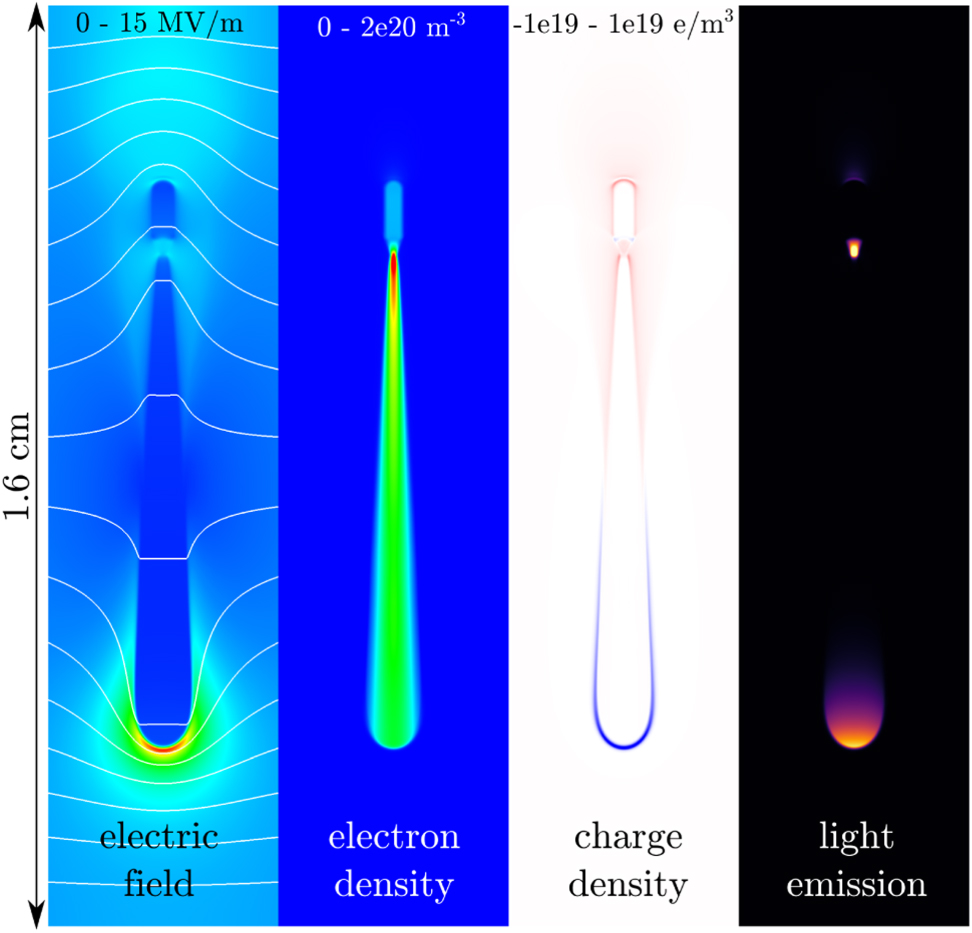
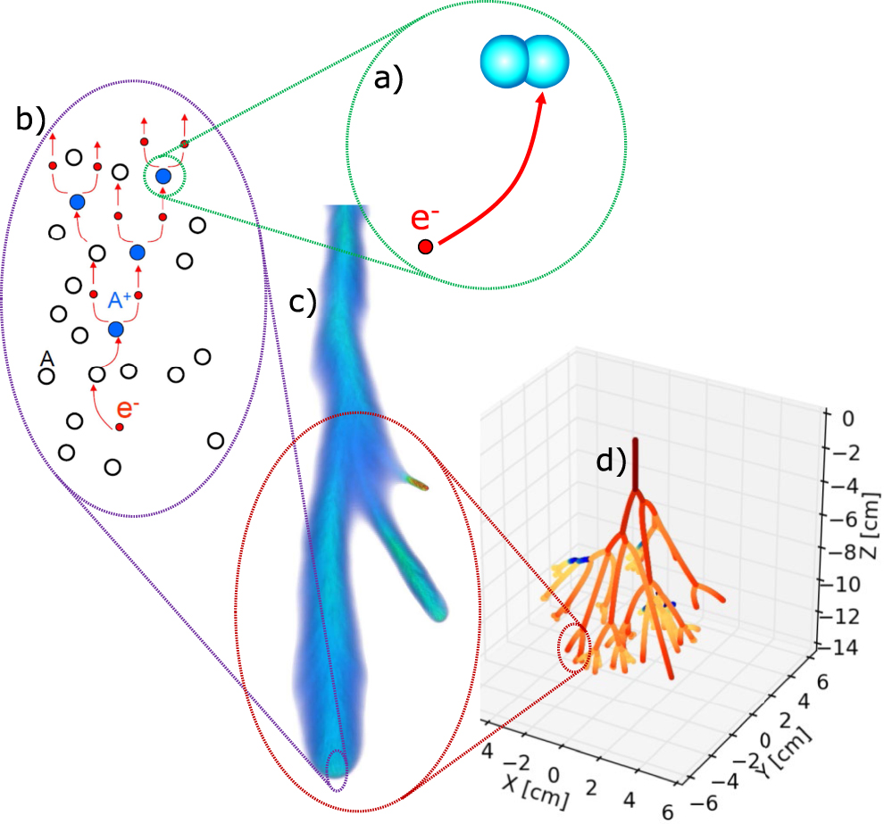
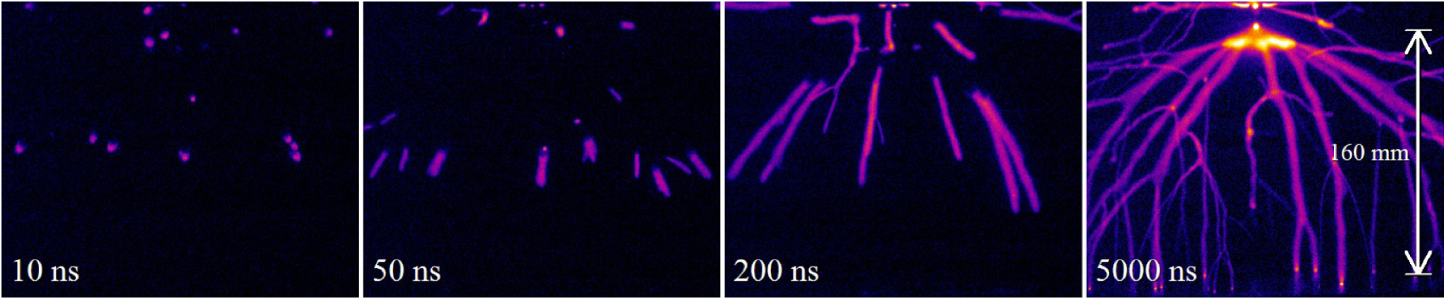
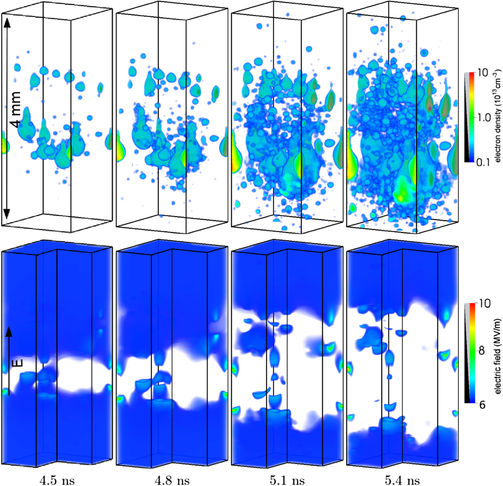
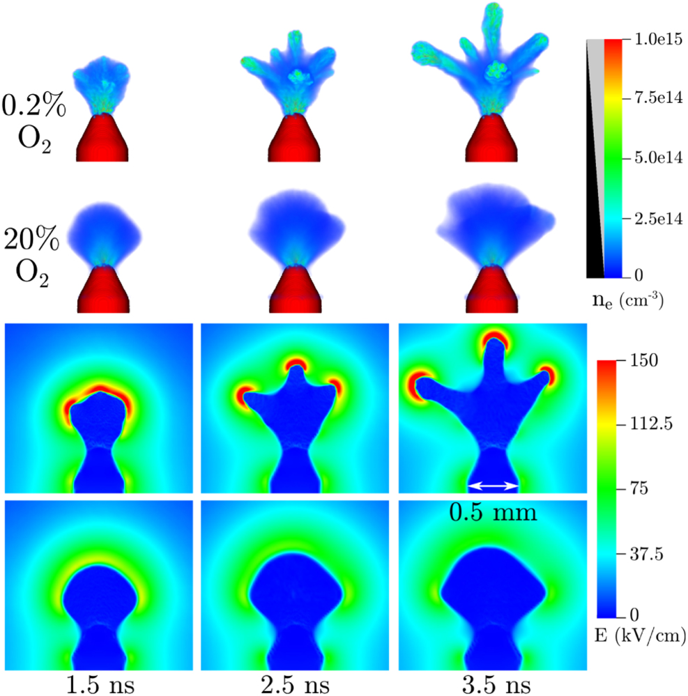
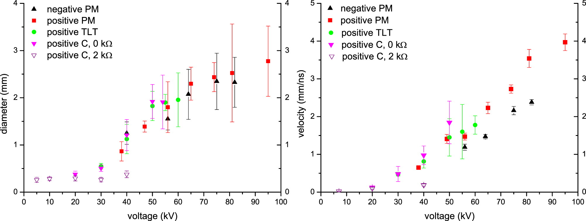
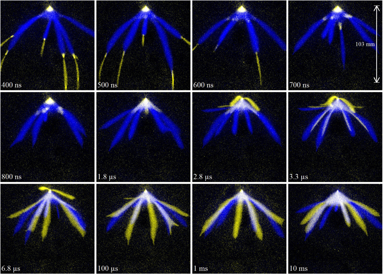
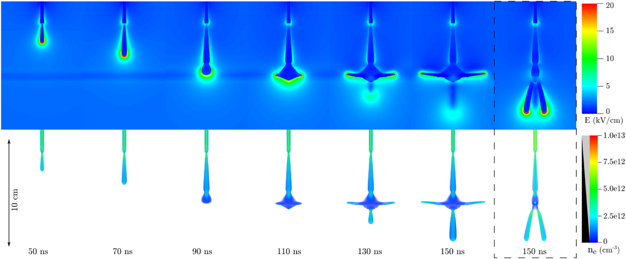
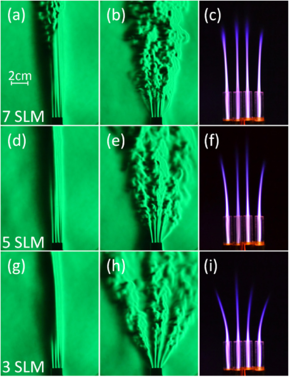
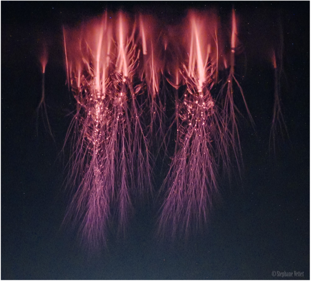
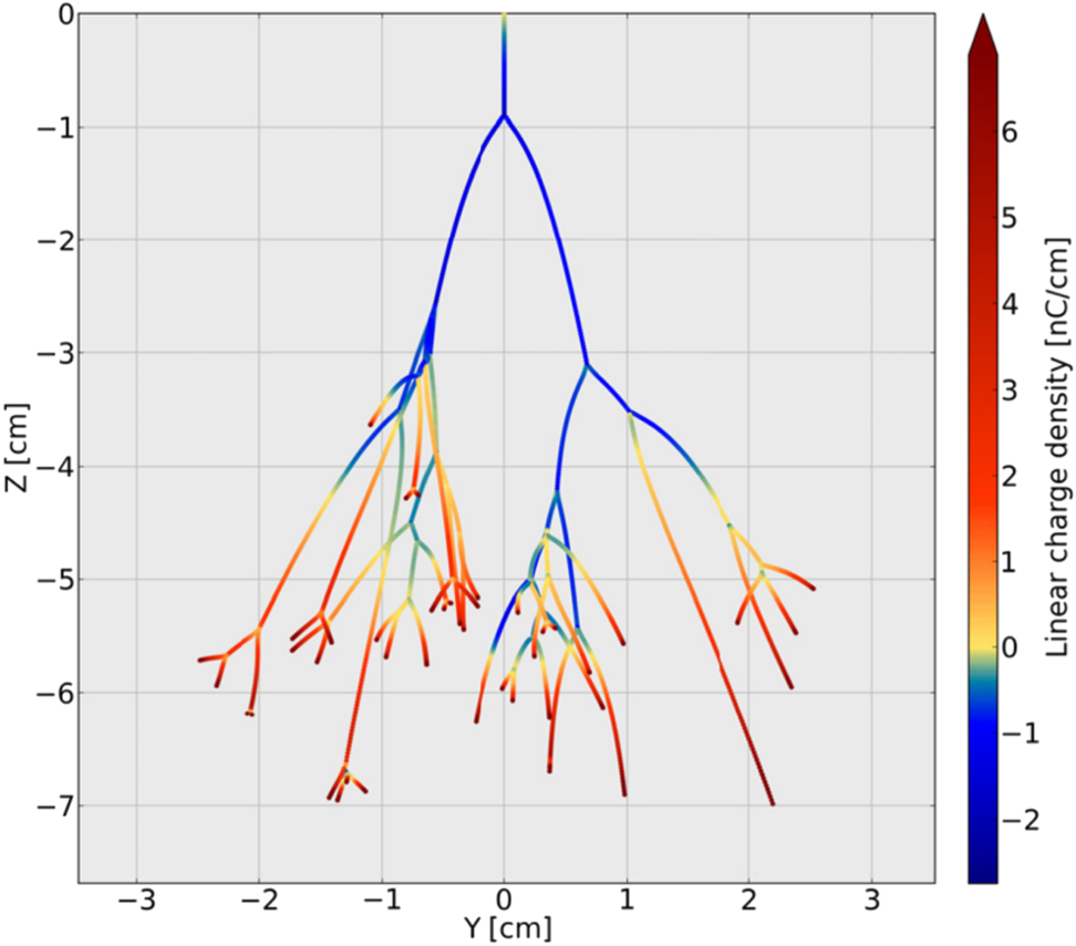
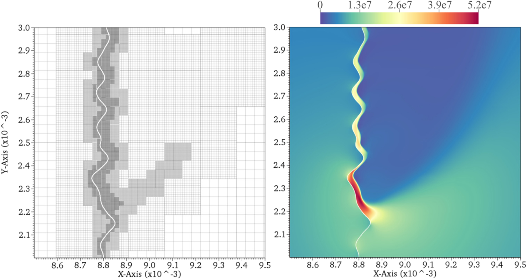
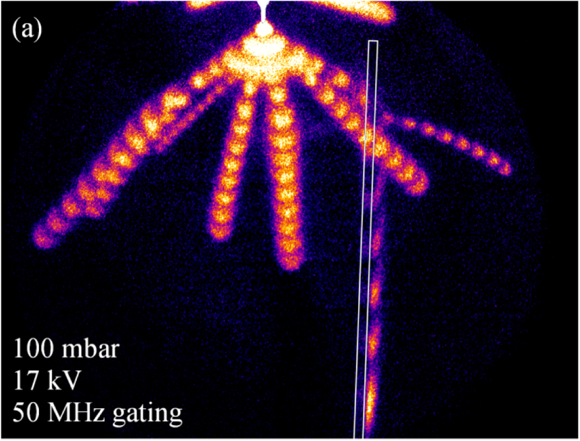
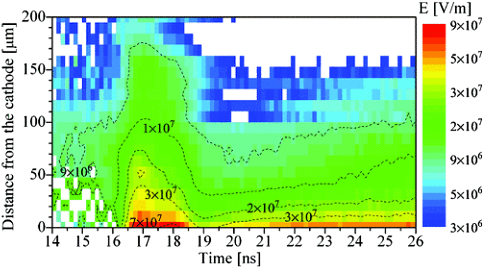
Figure 29. Two dimensional electron density distribution acquired by measuring refractive index variations. Image from [102].
Download figure:
Standard image High-resolution image
An upcoming diagnostic which can detect ions, ground-state neutrals, as well as most stable excited states all at once is mass spectroscopy. In particular molecular beam mass spectroscopy (MBMS) is a fast-developing technique [382–384] which has been shown to be able to quantify with high accuracy species like O3, NO [382], O−,  ,
,  [383] and singlet delta oxygen (O2(a1Δg)) [384]. MBMS is able to probe atmospheric pressure plasmas impinging on surfaces and can thereby detect the species at the location where the relevant surface chemistry takes place. Excited species are distinguished from each other and from ground state species by probing which energy is required to ionize them [384].
8. Outlook and open questions
We have reviewed our present understanding of streamer discharges, addressing basic physical mechanisms and observed phenomena. Our emphasis has been on positive streamers in air under lab conditions, whose properties like velocity, radius and maximal field already span a wide parameter space due to the progress of fast pulsed high-voltage sources.
We think that advances in diagnostic techniques and numerical modeling have brought a quantitative understanding of all streamer-related phenomena within reach. An important step in this direction will be the validation of numerical models. However, there are still many open questions regarding the physics of streamers, even when only considering positive streamers in air. Below, we have collected several of the most important ones. Our goal is to answer these questions, and to develop quantitative theories for streamer discharges that can be generalized to other gases or polarities.
8.1. Discharge inception
Section 2.1 and 2.3: which are the dominant electron sources for streamer inception in different parameter regimes, and for different polarities? What is the role of surfaces?
Section 2.2: which quantitative criteria for discharge inception can be developed beyond the classical Meek number criterion?
Section 2.4: does our proposed mechanism for the inception cloud also explain seemingly similar phenomena like 'diffuse discharges'?
Section 2.4: what determines the break-up of the inception cloud into streamers?
8.2. Streamer evolution
A particular problem is that most experiments show a burst of many branching streamers, whereas fluid or particle simulations become computationally very expensive when more than one streamer is present. Therefore, the overall discharge evolution cannot easily be compared, except if the experiment produces a single streamer, or if the microscopic models can be reduced to quantitative macroscopic tree models. To achieve the latter, the following questions need to be answered.
Section 3.2: can we understand the large range of velocities and radii of streamers in air for both polarities? How are they related to the local electric field and other conditions? Can this be described analytically from basic physics or only empirically from simulations and experimental results? Can the concept of coherent structures of section 1.2.5 help analyze the varying properties of streamer heads?
Sections 3.5, 3.8 and 6.4: can we understand the charge distribution in a streamer tree? What is the physical background of the experimentally often reported 'stability field'?
Section 3.9: what are the mechanisms causing streamer branching under varying conditions? Can we identify the distribution of branching lengths and angles?
Section 3.6: can we understand the stepped propagation of lightning leaders, and is this phenomenon related to streamers propagating in several bursts?
8.3. Further evolution after passage of ionization front
The reactions occurring after the passage of a streamer front depend strongly on the gas composition, so answers on the questions below can and will also vary with gas mixture.
Section 5.2: which plasma chemistry is precisely triggered by streamers? How does it depend on velocity, electric field and radius of the streamer head? How does this influence discharge evolution and how can it best be used in applications?
Section 5.3.2: what is the interaction between a streamer corona and a leader and what is the role of gas heating?
Section 3.4: how is conductivity in a streamer channel maintained? What are the roles of heating, plasma chemistry and the detachment instability? Are there nonlinear self-enforcing mechanisms in the streamer channel?
8.4. Particular physical mechanisms
Section 5.4: in which parameter regime of negative discharges do electron runaway and bremsstrahlung become important? Can they play a role in positive discharges as well?
Section 5.4: can electrons be accelerated in streamer discharges to energies that are possibly far higher than electrostatic acceleration would predict?
Section 5.4: can runaway electrons have a significant influence on streamers and, if so, how?
Section 4.1: is there photo-ionization or are there other substitutes for it in gases different from air? Why do we see widely varying streamer diameters for positive streamers in air but not in gases like pure nitrogen?