

Abstract
Properties of atmospheric pressure plasmas sustained by a 5 kHz pulse power are investigated by adjusting the duty cycle from 10% to 80%. As a result of the decrease of the duty cycle, the upward trends are observed in the electron density and excitation temperature, however, the downward trend appears in the gas temperature. The spatially averaged model is applied to simulate the temporal evolutions of the electron density and temperature, further validated by the time-resolved experimental measurements. Since the discharge volume in the open-air conditions increases at higher duty cycles, the time-averaged electron density within the pulse-on period consequently declines. For shorter duty cycles, fewer charges remain for the next discharge, and a higher initial peak of the electron temperature appears. As a result, the time-averaged electron temperature within the pulse-on period increases. Both the experimental and simulation results suggest that the discharge volume of the atmospheric pressure plasma in the open air has a strong effect on the time-averaged electron density during the pulse-on period whereas the remnant electron density determines the time-averaged electron temperature within the pulse-on period. This work reveals the effective mechanisms for controlling the electron temperature and electron density of atmospheric pressure plasmas in open air by using short pulse driven discharges.
Export citation and abstract BibTeX RIS
1. Introduction
Stimulated by the desirable advantages of more prominent non-thermal equilibrium, higher production efficiency of the reactive species and less power consumption compared to DC or sinusoidal driven plasmas [1–3], significant advances in research and industrial applications of atmospheric pressure plasmas generated in pulsed discharges have recently been reported [4–7]. Among the numerous factors that determine the properties of the pulsed discharge plasmas, the duty cycle is a critical one, and it can be controlled by adjusting the pulse duration or repetition rate. This is why exploring the role of the duty cycle in the generation and sustaining of pulsed discharge plasmas has become increasingly important. For example, Adams et al [8] found that the remnant energy left from the previous discharge pulse causes a significant gas temperature increase on the next pulse. Hsu and Wu [9] attributed the mode transition (from the glow discharge to the arc discharge) in pulsed atmospheric pressure plasma to the variation of pre-transition energy, thermal effect and discharge kinetics. Sun et al [10] found that the increase of duty cycle increases the number of discharge channels and favors the diffusion of ions to eliminate the uneven distribution of the plasma density, contributing to the more homogeneous plasma. Moreover, Kettlitz et al [11] compared the breakdown properties of a series of pulse driven dielectric barrier discharges at three duty cycles and concluded that the rest periods between the adjacent discharges affect the breakdown characteristics by determining the charge deposition at the dielectric surface.
These papers have covered various pulsed discharge forms, but are short of explorations about the mechanisms of how the duty cycle determines the properties of the pulsed discharge plasmas, especially for the two vital parameters: the electron temperature and density. For this purpose, here we study the excitation temperature and electron density at different duty cycles and find that a short duty cycle is beneficial to improve both the excitation temperature and electron density of the atmospheric pressure plasma. The numerical simulations are also performed to explain the experimental results, and the simulation results are further validated by the time resolved measurements of the electron density and excitation temperature. This work reveals that the remnant electron density left by the previous pulse determines the time-averaged electron temperature by affecting the initial peak amplitude of the electron temperature. The electron density at different duty cycles is coupled with the change of the discharge volume in the open air.
2. Experiments and computational model
2.1. Experimental setup and V–I characteristics
The experimental setup is described in our previous article [12]. A platinum electrode immersed in saturated NaHCO3 solution acts as the anode, and a tungsten steel tube with an internal diameter of 1 mm acts as the cathode. Argon gas with flow rate of 50 sccm (Reynolds number: 75.57, laminar flow) is introduced into the tube as the working gas. The gap between the exit of the tube and the solution surface is adjusted to 2 mm. A high-voltage DC power source (SL2000, SPELLMAN) and a pulse generator (PVX-4110) are operated together to generate 2 kV amplitude and 5 kHz frequency pulses with the adjustable duty cycle to drive the circuit. To diagnose the excitation temperature and electron density, the optical emission spectrum (OES) and the images of the plasma are collected by a spectrograph (SP-2500, Princeton Instruments) and an intensified charge coupled device (ICCD, PI-MAX4, Princeton Instruments), respectively. An oscilloscope (Tektronix MDO3024) is used to monitor the discharge current and the voltage drop of the discharge. Figure 1 shows the waveforms of the discharge current, the voltage drop and the power absorbed by the plasma at each duty cycle. The discharge characteristics during the initial 0–3 μs are also presented in the inset of figure 1 with higher time resolution.
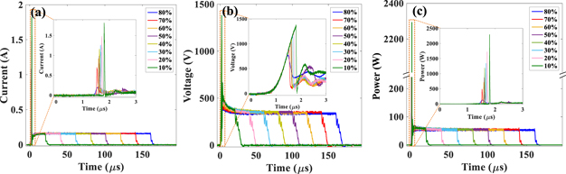
Figure 1. Waveforms of the discharge current, the voltage drop of discharge and the power absorbed by the plasma at each duty cycle. (a) Discharge current. (b) Voltage drop of discharge. (c) Power absorbed by plasma.
Download figure:
Standard image High-resolution imageAs shown in figure 1, the discharge combines the characteristics of pulsed discharges at the beginning of the pulse and DC discharges in the later phase. In detail, when the plasma is ignited, the breakdown voltage decreases by 44% (from 1380 to 776 V), the breakdown current sharply drops by 89% (from 1.82 to 0.2 A) and the peak power dramatically declines by 94% (from 2293 W to 124 W) when the duty cycle rises from 10% to 80%. Similar observation was reported in reference [13]. They speculated that fewer residual charges left from the previous discharge serve as the seed charges in the case of a short duty cycle, thus a higher breakdown voltage is required to ignite the plasma [13]. After the discharge reaching the steady state, the voltage drop and the discharge current for different duty cycles are both stabilized at 400 V and 150 mA, respectively, with the corresponding power of 60 W.
2.2. Electron density diagnostics
The electron density is diagnosed by the Stark broadening and imaging methods simultaneously. The Stark broadening in the optical emission lines is directly related to the electron density due to the large linear Stark effect of the electron density. It is thus a convenient and traditional way to diagnose the electron density by measuring the Stark broadening of the optical emission lines. Apart from the Stark broadening, the optical emission lines of the plasma are also broadened by multiple mechanisms including the van der Waals broadening Δλw, the instrumental broadening Δλi and the Doppler broadening ΔλD. After obtaining the gas temperature and the instrumental broadening [14, 15], the Stark broadening could be extracted from the optical emission lines, and then the electron density could be calculated [16, 17]. However, the major shortcoming of the Stack broadening method is the low limit of the electron density. If the electron density is lower than 6 × 1014 cm−3 for Hα line or 4 × 1013 cm−3 for Hβ line, the fine structure components (FSC) will be larger than the Stark broadening contribution and it is hard to extrapolate the Stark width from each FSC [17, 18]. Moreover, the Stark broadening at the full width of half maximum (FWHM) Δλs of Hβ line is the common function of electron temperature Te and electron density ne. The relationship was fitted by Czernichowski and Chapelle [19] and is expressed as:
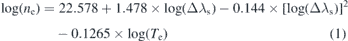
where ne is in m−3, Δλs is in nm and Te is in K. Equation (1) is valid for 3.16 × 1014 cm−3 ⩽ ne ⩽ 3.16 × 1016 cm−3 and 5000 K ⩽ Te ⩽ 20 000 K. Figure 2(a) shows the relationship between ne, Te and Δλs based on equation (1). It is clear in figure 2(a) that if ne < 1015 cm−3, the dependence of Δλs on Te is so weak that Δλs could be regarded as the only function of ne, which could be calculated by [16]:

Here, ne is in cm−3, Δλs is in nm and ne > 1014 cm−3. While if ne > 1015 cm−3, the dependence of Δλs on Te is stronger so that Δλs is not suitable for the electron density diagnostics. As a complementary tool, the Stark broadening at the full width of half area (FWHA)  of Hα line (defined in report [16]) relies only on the electron density but not on the electron temperature. Therefore, for the case of large electron density (ne > 1015 cm−3),
  of Hα line is a better choice to measure the electron density based on equation (3) [17]:

Here, ne is in cm−3,  is in nm and ne must be larger than 5 × 1014 cm−3. The examples of the Hβ line and Hα line fitting used in the Stark broadening method are shown in figures 2(b) and (c), respectively.
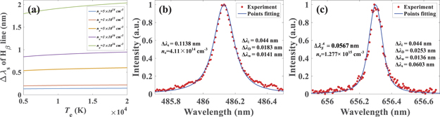
Figure 2. Electron density diagnosed by the Stark broadening method. (a) Relationship between ne, Te and Δλs. (b) Hβ line fitting. (c) Hα line fitting.
Download figure:
Standard image High-resolution imageAnother electron density diagnostic method is the imaging method, which is based on the relationship between the electron density and the plasma inductance [12]. It is not limited by the lower limit of the electron density while the plasma sizes can also be obtained, simultaneously. Nevertheless, this method is only applicable for the stable discharge conditions. The limited ability to diagnose the electron density at the breakdown time is its weakness compared with the Stark broadening method. Figure 3(a) displays the plasma images used in the imaging method with the calculated plasma sizes shown in figure 3(b). Observing the images in figure 3(a) from 10% to 80%, it looks like the evolution of discharge from the streamer plasma column filling the whole gap towards the glow discharge with a bright space near the cathode and a dark space in the rest of the gap. As seen in figure 3(b), the plasma swells with the radius increasing from 0.23 to 1.1 mm while the plasma length remains almost unchanged at the gap distance 2 mm when the duty cycle is varied from 10% to 80%.
Figure 3. Size and electron density diagnosed by the imaging method. (a) Normalized spatially resolved emission intensities (plasma images) at different duty cycles. (b) Plasma sizes at different duty cycles.
Download figure:
Standard image High-resolution image2.3. Temperature diagnostics
In the atmospheric pressure environment, the determination of electron temperature Te is always based on the diagnostic of excitation temperature Texc because Texc has the same tendency as Te when the discharge parameters are varied [20, 21]. Assuming that the upper energy levels of the atomic transitions satisfy the local thermodynamic equilibrium condition, namely the population density of these levels follows the Boltzmann distribution, the Boltzmann plot method [22, 23] could be employed to determine Texc of the plasma according to the expression given by:

where λij and Iij are the wavelength and relative intensity of the OES between the upper level i and lower level j, respectively. Here, gi is the statistical weight of the upper level i, Aij is the transition probability from level i to level j, Ei is the excitation energy of level i, k is the Boltzmann constant and C is a constant. Figure 4(a) shows the selected ArI spectral lines of 4p–4s and 5p–4s transition. Referring NIST atomic database [24], Texc is obtained from the slope of the straight line by linearly fitting the left-hand side of equation (4). An example of the fitting result of Texc is shown in figure 4(b).
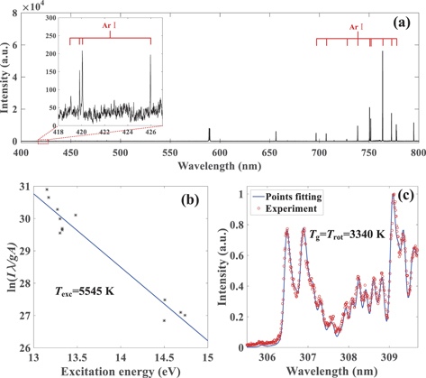
Figure 4. Measurements of excitation temperature and gas temperature. (a) Selected ArI spectrum of 4p–4s and 5p–4s transition lines. (b) Linear fitting of the excitation temperature. (c) Fitting of the OH(A–X) emission bands from 305.5 nm to 309.75 nm.
Download figure:
Standard image High-resolution imageAs for the gas temperature Tg, it is estimated by calculating the rotational temperature Trot of the plasma [25, 26], which could be determined by fitting the OH(A–X) emission bands from 305.5 nm to 309.75 nm [27]. This fitting is achieved by the simulation software LIFBASE [28] with an example shown in figure 4(c).
2.4. Computational model
The spatially averaged model [29–33] is applied to evaluate the two most important plasma parameters: electron temperature and electron density. There are two ways to create electrons in the gas discharge: atomic or molecular ionization and the secondary electron emission. The former is resulted from the collisions between electrons and neutral atoms or molecules, and the latter is due to the positive ions bombarding the cathode. While electron acceleration towards to the anode is the main channel of the electron loss. Therefore, the temporal dynamics of the electron density can be described by the electron balance equation:

In equation (5), the electron density changing rate in the bulk depends on the ionization rate νiz of the neutral particles and the electron loss rate νloss, where νiz = ngKiz and νloss = uB/d. Here, ng is the density of specific gas, Kiz is the ionization rate coefficient for specific gas, γse is the secondary electron emission coefficient and uB is the Bohm velocity.
The power source is a rectangular wave and the power absorbed by the plasma could be regarded as a constant P within the pulse-on period. Using the spatially averaged model, the complete power balance equation is expressed as:
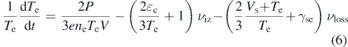
where ɛc is the energy consumption to create a new electron–ion pair, Vs is the sheath voltage and V is the discharge volume of the plasma. Based on equations (5) and (6), the schematics of the temporal evolution of Te(t) and ne(t) for a fixed discharge volume during the whole pulse period are presented in figure 5. Similar variations are also observed in the simulations [30, 31] and experiments [33].
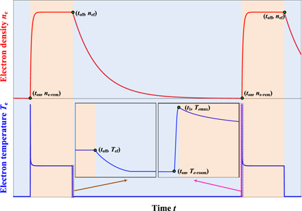
Figure 5. Schematic of the time dependence of the electron density and electron temperature when the discharge volume is fixed. (The blue and orange background represent the off and on phases of the pulse, respectively.)
Download figure:
Standard image High-resolution imageWhen the power source is turned off at t = toff, P in equation (6) equals to zero. During the pulse-off period, both the electron density and the electron temperature decrease gradually as shown in figure 5. It can be seen that the electron temperature decreases straight down to the room temperature Te–room (0.026 eV), while the electron density also continually falls until the next pulse is turned on; at this point of time the remnant electron density is denoted as ne–rem.
Once the power source is turned on at t = ton, steep ascending slopes are observed in Te and ne. Because of the time delay between two processes, i.e. electron gaining energy from the electric field and electron ionizing the neutral particles, Te increases more rapidly than ne. With Te increasing, ne grows and dTe/dt in turn declines. When t = t1, dTe/dt = 0 and Te = Temax. Subsequently, because of the still-growing ne, Te begins to decrease until it reaches the final stationary value Tef, while ne continues to increase until arriving at its stationary value nef. At the time when dTe/dt = 0 and dne/dt = 0, the discharge reaches the steady state with Tef and nef being described by equations (7) and (8) where ɛc ≫ Te [34] and Vs ≫ Te [29].


Considering the actual situation of the experiments, although the feed gas is pure argon, when the discharge is exposed to air, the impurity gases, such as oxygen and nitrogen are inevitable to permeate the argon. Therefore, apart from the argon atoms ionization (e + Ar → Ar+ + 2e), the oxygen molecular ionization (e +  + 2e, e + O2 → O + O+ + 2e) and nitrogen molecular ionization (e +
  + 2e) should also be considered so that the total νiz–total in equation (5) is given by:

In equation (9), i represents the gas species, including the ground-state Ar, N2 and O2. Here, we ignore the ionization of the ground-state nitrogen and oxygen atoms, metastable argon atoms, nitrogen and oxygen molecules as well as the oxygen negative ions due to their much lower density compared with the original ground-state carrier gas in the atmospheric pressure environment [31]. However, the dissociative attachment (e + O2 → O + O−) of oxygen molecules should be taken in consideration. The formation of negative ions O− consumes the electron density and significantly affects the electron density during not only the pulse-on phase but also the pulse-off phase. Therefore, the total νloss–total in equation (5) is rewritten as:

where  is the dissociative attachment rate coefficient of oxygen molecular. In this case, the electron balance equation (5) is changed to:

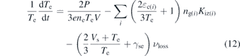
Additionally, if the air impurity is taken in account, the power balance equation (6) should also be changed to:
From equations (9)–(12), the rate coefficients Kiz(i),  and the energy loss ɛc(i) are adopted from the previous reports for argon [34], for nitrogen [35] and for oxygen [36] with the suitable range of 1 eV ⩽ Te ⩽ 7 eV. Moreover, the other input parameters include: P = 60 W, Vs = VDC = 400 V as shown in figure 1 and γse = 0.1 [37], which is typically achievable in capacitive coupled plasmas. The total gas density (ng(Ar) +
  +
+  ) is 2.6875 × 1025 m−3 under the atmospheric-pressure conditions and the plasma volume V at different duty cycles is based on the calculation results in figure 3(b).
3. Results and discussion
The electron density at different duty cycles within the pulse-on period was diagnosed by the imaging method and the Stark broadening method and is presented in figure 6(a). It can be seen that the electron density measured by the imaging method and the Stark broadening method are consistent with each other and collectively indicate that the electron density decreases from 4.04 ×10¹⁴ to 4.36 × 1013 cm−3 as the duty cycle increases from 10% to 80%. In this case, using the Stark broadening method based on the Hα line is not accurate in this electron density range. Additionally, in view of the low accuracy of the Stark broadening method when the electron density is lower than 1014 cm−3 is to be fitted by Hβ line [16], the data measured by the Stark broadening method at the duty cycle higher than 50% are drawn by a dashed line. The excitation temperature and the gas temperature versus the duty cycle are both shown in figure 6(b). With the duty cycle increasing from 10% to 80%, the excitation temperature decreases from 9100 to 5200 K, while the gas temperature rises from 2750 to 3910 K. Obviously, the excitation temperature and the gas temperature gradually approach to each other as the duty cycle becomes larger. Due to the intense heat exchange between the electrons and the carrier gas via inelastic collisions, the plasma is closer to the thermal equilibrium state when the pulse duration is longer.
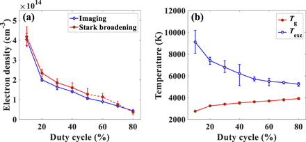
Figure 6. Diagnosed results of the plasma parameters at different duty cycles. (a) Electron density. (b) Excitation temperature and gas temperature.
Download figure:
Standard image High-resolution imageThe simulated steady state electron density nef versus the duty cycle under different argon purities is shown in figure 7(a). For reference, the diagnosed electron density given in figure 6(a) is also superimposed on figure 7(a). A remarkable deviation of the diagnosed electron density from the simulated nef evidences that the discharge gas is not pure argon. If 0.2%–0.6% air (N2:O2 = 4:1) addition is considered in the simulation, the discrepancy could be reduced and the simulated nef becomes consistent with the experimental results. It can be explained by noting the additional electron energy losses in collisions leading to rotational and vibrational excitation of O2 and N2 [38], which significantly increases the total energy loss to create new electrons, even if a tiny amount of air is permeated into argon. The simulated Te–room and Tef under different argon purities and duty cycles are both plotted in figure 7(b). It is clear that both of Te–room and Tef keep unchanged when the duty cycle increases from 10% to 80%, while Tef slightly increases from 1.27 eV to 1.417 eV (corresponding Texc rises from 4779 K to 4919 K [21]) when the air addition rises from 0% to 1%.

Figure 7. Simulated plasma parameters at different duty cycles and argon purities. (a) Electron density in the steady state. (b) Electron temperature in the steady state (solid line) and pulse-off period (dotted line).
Download figure:
Standard image High-resolution imageIn general, since both of the exposure time of the ICCD and the integration time of the spectrometer for each duty cycle match the pulse duration, the experimental results are actually the time-averaged values of electron temperature ⟨Te⟩ and electron density ⟨ne⟩ during the pulse duration. Comparing figure 6(a) with figure 7(a), it can be seen that the variation trend of the diagnosed (time-averaged) electron density is in agreement with that of the simulated electron density in the steady state. This result indicates that the duty cycle dependence of the electron density in the steady state plays a dominant role in the variation of the time-averaged electron density ⟨ne⟩ versus the duty cycle. Additionally, the remnant electron density ne–rem is much lower than the electron density in the steady state and has no significant effect on ⟨ne⟩. Since the discharge current in the steady state is the same for different duty cycles, one can expect that it is the variation of the discharge volume dependent on the duty cycle as shown in figure 3(b) that results in the changes of ⟨ne⟩ versus the duty cycle according to equation (8).
In comparison of figure 6(b) with figure 7(b), it can be seen that Te–room and Tef are independent of the duty cycle. However, the experimental results show that the time-averaged electron temperature ⟨Te⟩ decreases as the duty cycle rises. Therefore, one can expect that the electron temperature in the time region before the plasma arrives at steady state is a function of duty cycle and has a strong effect on ⟨Te⟩. To clarify this effect, the temporal evolutions of the electron density and the electron temperature at different duty cycles are investigated.
Differently from the simulation in the ideal discharge environment shown in figure 5, the actual gas composition, power absorption and the plasma volume should be considered together to reproduce the experimental conditions accurately. From figure 6(a), one can see that the diagnosed line is almost between the simulated nef lines corresponding to 0.2% and 0.6% air addition. Here, we choose the average ratio of 0.4% as the air addition in the following simulations. In figure 1(c), the power peak at the breakdown moment also affects the simulation results, so that the actual absorbed power P(t) derived from figure 1(c) is used in equation (12) instead of P = 60 W. The temporal plasma images at the duty cycle from 60% to 80% are recorded with the time resolution of 20 μs and displayed in figure 8(a). Applying the imaging method, the corresponding plasma volumes are calculated and plotted in figure 8(b).

Figure 8. Temporal evolutions of plasma image and volume at the duty cycle from 60% to 80%. (a) Normalized spatially resolved emission intensities (plasma images). (b) Calculated plasma volumes by the imaging method.
Download figure:
Standard image High-resolution imageFrom figures 8(a) and (b), one can see that the plasma is brighter and the volume is a little larger at the initial 20 μs than that at other times for each duty cycle. However, the plasma volumes are almost invariable after 20 μs although there is a little fluctuation (<9%). This is because the transient breakdown occurs during the initial 20 μs period, when most of the excited atomic species are produced, and their subsequent decay results in intense light emission [39]. The experimental results in figures 3(a) and 8(a) indicate that the plasma volume strongly depends on the duty cycle but much weaker on time except the breakdown moment. Therefore, it is reasonable to assume that the plasma volume does not change with time when the discharge is stable. Nevertheless, at the start of the discharge, the larger plasma volume in figure 8(b) should be considered in the simulation.
Under the conditions mentioned above, the remnant electron density at different duty cycles is first obtained based on the simulated nef and Tef in figure 7 and is shown in figure 9(a). The temporal evolutions of the electron density and electron temperature at the duty cycles of 60%, 70% and 80% are presented in figures 9(b)–(e). In detail, figures 9(b) and (c) plot the temporal evolution of the electron density during the pulse-off and pulse-on periods, respectively, where the electron density at the end of the pulse-off time is given in the inset of figure 9(b) with higher time resolution. Likewise, figures 9(d) and (e) present the temporal evolution of the electron temperature during the pulse-off and pulse-on periods, respectively, where the electron temperature at the start of the pulse-off time is shown in the inset of figure 9(d) with higher time resolution. Here we assume that the reaction rate coefficients involving Ar, N2 and O2 are all valid for the range 0.026 eV ⩽ Te ⩽ 10 eV.
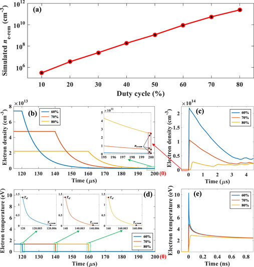
Figure 9. Simulation results of the spatially averaged model. (t = 0 is the time when the breakdown happens.) (a) Remnant electron density. (b) Temporal evolution of electron density at the pulse-off moment. (c) Temporal evolution of electron density at the pulse-on moment. (d) Temporal evolution of electron temperature at the pulse-off moment. (e) Temporal evolution of electron temperature at the pulse-on moment.
Download figure:
Standard image High-resolution imageFrom figures 9(a) and (b), it can be seen that although the electron density in the steady state increases, the remnant electron density after the pulse-off period goes down when the duty cycle is decreased. This result can be explained by noting that there is more time for the electron density to relax when the duty cycle is decreased, thus leading to the declining remnant electron density. Differently from figure 9(b), the electron temperature after the pulse-off period is the same at different duty cycles as shown in figure 9(d). This is due to the fact that it takes only 6 ns for the electron temperature to drop to room temperature and then remain unchanged. The remnant electron density together with the initial energy (room temperature) is the initial condition of the next discharge, which plays an important role in the temporal evolution of the electron temperature and the electron density in the next discharge. In the case of a short duty cycle, under the influence of the higher transient peak power and lower remnant electron density, each electron can gain more energy from the electric field. These high-energy electrons also accelerate the ionization of the neutral gas so that a peak of the electron density corresponding to the power (current) peak at the beginning of each pulse is observed in figure 9(c). Figure 9(e) shows that the electron temperature rises to the peak value and then relaxes to the stationary value gradually, which indicates that the discharge is in the steady state for most of the time during the pulse-on period. Nevertheless, the transient value of the electron temperature before plasma relaxing to the steady state is too high to be ignored in considering the time-averaged electron temperature ⟨Te⟩ within the pulse-on period. Since the transient electron temperature before the plasma relaxing to the steady state decreases versus the increase of the duty cycle, ⟨Te⟩ during the pulse-on period decreases at higher duty cycles as shown in figure 6(b). Likewise, the electron density peak also increases ⟨ne⟩, but compared with the discharge volume, which determines nef directly, this effect is negligible.
To verify the simulation results shown in figure 9, especially the initial phases of the pulse-on period in figures 9(c) and (e), experiments with higher time resolution (0.5 μs) are conducted to observe the temporal evolutions of the electron density and excitation temperature during the first 5 μs after the moment of breakdown. Based on the simulation, shorter duty cycles produce more obvious variations of ne and Te. Considering the measurement limitations of the electron density for Balmer lines, we select the duty cycle of 20% for the following experiments.
The temporal evolution of the electron density diagnosed by the imaging method and the Stark broadening method at 20% duty cycle are presented in figure 10(a). Noting that the imaging method is not accurate at the breakdown time when the discharge is unstable, the imaging method is not applied during the first 1 μs. When t < 2 μs, ne > 5 × 1014 cm−3, the FWHA of Hα line is suitable to diagnose the electron density, and for t > 2 μs, ne is relatively lower so that the FWHM of Hβ line can be used. The experimental results in figure 10(a) show that the electron density decreases from 1.24 × 1016 cm−3 at 0 μs to 2.29 × 1014 cm−3 at 5 μs rapidly. The observed trend is in an agreement with the simulation results in figure 9(c) and the experimental results [40]. Figure 10(b) displays the temporal evolutions of excitation temperature Texc and gas temperature Tg. One can see that Texc decreases from 12 120 K to 7820 K during 0–5 μs. This trend is also consistent with the simulation results in figure 9(e). Meanwhile, Tg increases from 2190 K to 3210 K during this period. The similar results between the time resolved experiments and simulation corroborate that our model is reliable, and it is expected that shortening the pulse duration is favorable to improve the electron temperature and electron density of the plasma in ambient conditions.

Figure 10. Temporal evolution of the plasma parameters during the first 5 μs after the breakdown moment (t = 0 μs). (a) Electron density. (b) Excitation temperature and gas temperature.
Download figure:
Standard image High-resolution image
4. Conclusion
In this work, the influence of the duty cycle on the atmospheric pressure pulsed plasma is investigated. The experimental results show that both the electron density and excitation temperature increase but the gas temperature decreases when the duty cycle is increased. As the energy is transferred from the electric field to the plasma, the numerical simulations based on the spatially averaged model are applied to describe the temporal evolution of the electron temperature and the electron density. During the pulse-on period, a peak of the electron density corresponding to the current peak appears after the plasma is generated and gradually decreases to the stationary electron density when the plasma reaches the steady state. During the pulse-off period, the electron density decreases gradually to the remnant electron density until the start of the next pulsed-on period. Since the discharge volume is enlarged, the electron density of the plasma in the steady state decreases when the duty cycle is increased. Consequently, the time-averaged electron density within the pulse-on period decreases. Because there is less time for the electron density to relax, the remnant electron density increases with the increase of the duty cycle. The remnant electron density plays an important role in the temporal evolution of the electron temperature. During the pulse-on period, the electron temperature increases rapidly to the peak value just after the plasma is generated, and then gradually declines to the stationary value, which is independent on the duty cycle. During the pulse-off period, the electron temperature drops quickly to the room temperature. When the duty cycle is shortened, the lower remnant electron density leads to the electron temperature increase faster to the higher peak value. These factors contribute to the increase of the time-averaged electron temperature within the pulsed-on period.
In summary, when the duty cycle is reduced, the discharge volume of the plasma in the open-air environment decreases and effectively boosts the steady state electron density, which leads to the higher time-averaged electron density. Meanwhile, the pulse-off period is prolonged by reducing the duty cycle and results in the lower remnant electron density. The lower remnant electron density leads to the rise of the initial electron temperature once the plasma is generated, which in turn increases the time-averaged electron temperature.
Acknowledgments
This work is supported by the National Natural Science Foundation of China (NSFC) (Grant No. 11675109) and the National Key Research and Development Program of China (No. 2018YFA0306304). KO thanks the Australian Research Council for partial support.