
Abstract
We here propose to model the production of energetic electrons serving as a source of x-rays and γ-rays, associated to electric discharges in preionized and perturbed air. During its stepping, the leader tip is accompanied by a corona consisting of multitudinous streamers perturbing the air in its vicinity and leaving residual charge behind. We explore the relative importance of air perturbations and preionization on the production of energetic runaway electrons by 2.5D cylindrical Monte Carlo particle simulations of streamers in ambient fields of 16 and 50 kV cm−1 at ground. We explore preionization levels between 1010 and 1013 m−3, channel widths between 0.5 and 1.5 times the original streamer widths and air perturbation levels between 0% and 50% of ambient air. We observe that streamers in preionized and perturbed air accelerate more efficiently than in non-ionized and uniform air with air perturbation dominating the streamer acceleration. We find that in unperturbed air and in fields above breakdown strength preionization levels of 1011 m−3 are sufficient to explain significant runaway electron rates. In perturbed air, the production rate of runaway electrons varies from 1010 to 1017 s−1 with maximum electron energies from some hundreds of eV up to some hundreds of keV in fields above and below the breakdown strength with only a marginal effect of the channel radius. Conclusively, the complexity of the streamer zone ahead of leader tips allows explaining the emission of energetic electrons and photons from streamer discharges in fields below and above the breakdown magnitudes.
Export citation and abstract BibTeX RIS

Original content from this work may be used under the terms of the Creative Commons Attribution 4.0 licence. Any further distribution of this work must maintain attribution to the author(s) and the title of the work, journal citation and DOI.
1. Introduction
In 1994 the burst and transient source experiment on the Compton Gamma ray observatory was the first to measure beams of high-energy photons emitted from thunderstorms [1]. These bursts of X- and γ-rays have photon energies ranging from several eV up to at least 40 MeV [2] and last from hundreds of microseconds [3]) up to minutes [4]. Their existence and properties have been confirmed and refined by later missions (see e.g. [3, 5–7]) and are subject to the contemporary atmosphere-space interactions monitor (ASIM) [8] and the upcoming Tool for the Analysis of RAdiation from lightNIng and Sprites (TATANIS) missions [9] with payloads dedicated to the measurement of optical and high-energy radiation emitted from thunderstorms.
Whereas it is known that these photons are Bremsstrahlung photons from energetic electrons (e.g. [10, 11] and citations therein), so-called runaway electrons [12, 13], it has not been fully understood yet how electrons are accelerated into the energy range where they are capable of producing photons from keV to tens of MeV. Whilst electrons are energized by the thunderstorm electric fields, they collide in turn with air molecules and lose energies due to inelastic collisions. Hence, there is an interplay between the electron acceleration and the deceleration determining the characteristic electron energy distribution function.
The generation of runaway electrons is a stochastic process. However, its essence and magnitudes can be explained in terms of a conventional deterministic approach considering the simple case of a homogeneous electric field E [13–20]. While electrons with energy Ekin move in a dense gas medium, they experience a drag or friction force F(Ekin) as a result of inelastic (ionization, excitation, radiative losses) interactions with air molecules. In this deterministic approach, a drag force is introduced as a continuous function of the electron energy Ekin, for which either the Bethe equation [13, 19] or more accurate semi-empirical equations [14, 17–20] are used. Using such continuous functions below approximately 100 eV, instead of stepwise energy losses, is not correct since the lost energy is comparable to the energy before the interaction. The friction force has one maximum and one minimum, which are equal to Fmax ≈ 27 MeV m−1 at Ekin,max ≈ 150 eV and Fmin ≈ 218 keV m−1 at Ekin,min ≈ 1 MeV in air at standard temperature and pressure (STP). Above Ekin,min, the function F(Ekin) slowly increases up to ultrarelativistic energies where radiative losses dominate.
There are currently two possible theories explaining the production of high-energy runaway electrons in kilometer long lightning discharges and thunderclouds: the continuous acceleration and multiplication of high-energy electrons, remnants from cosmic rays, in the large-scale uniform thundercloud electric fields [21–24] or the acceleration of low-energy electrons in the high-field regions localized close to lightning leader tips [25–28], both including the feedback of Bremsstrahlung photons and of pair-produced positrons and electrons [29–33].
The formation and propagation of lightning leaders is mediated by a multitude of streamer channels, as depicted in figure 1. The importance of these streamers on the production of runaway electrons is manifold: Past models have indicated that electrons might be accelerated into the runaway regime by the high electric fields at the streamer tips [26, 27] and further be accelerated by the electric field of the lightning leader during its stepping process. Yet, the environment of the leader tip is very complex, and there are currently no self-consistent models that consider the influence of the streamer zone onto the environment of the leader tip (figure 1(a)). Furthermore, Cooray et al [34] suggested that the electric field might significantly be enhanced during the encounter of two streamers. This is supported by simulations by Luque [35] whereas simulations by Ihaddadene and Celestin [36] and Köhn et al [37] have shown that the duration of the field enhancement is too small to contribute significantly to the production of runaway electrons.
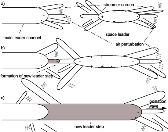
Figure 1. The leader stepping mechanism including air perturbation and preionization: (a) ahead of the main leader channel and around the space leader, coronas form consisting of a multitude of streamers which ionize and perturb surrounding air. (b) Two streamers of the main leader channel and of the space leader connect and trigger the formation of a new leader step. (c) After the potential from the tip of the previous main leader channel has been transformed to the tip of the new leader, streamers from the new tip move in perturbed (illustrated by waves) and preionized air.
Download figure:
Standard image High-resolution imageAdditionally, streamers support the propagation of lightning leaders. Several observations have indicated the stepping pattern, a discontinuous propagation mode, of lightning leaders [38, 39]. Whilst the exact mechanism of leader stepping is still under debate, the current apprehension combines the stepping with existence of the so-called space stem [40] and the streamer corona. After the leader motion has paused, a dipole called space stem or space leader manifests several tens of meters away [41]. Subsequently, streamer coronae originate from the leader tip and from both poles of the space stem (figure 1 (a)). This enables the reconnection of the two streamer coronas facing towards each other resulting in a leader step (figure 1(b)). Afterwards a new conducting channel is formed with the electric potential of the old leader transferred to the former space stem. This potential drop releases a new ionization wave becoming manifest as a streamer propagating into the preionized channel created from the streamer corona of the space stem averted from the leader tip side (figure 1(c)). Experiments [42] and simulations of streamers in uniform preionization [43] have shown that newly incepted streamers in the above-mentioned scenario move in a preionized channel with a decay length similar to the decay length of the streamer. Babich et al [27] have shown that for preionization densities between 1010 and 1015 m−3, the production of runaway electrons is enhanced compared to the production of runaway electrons by streamers in non-ionized air.
Along with the acceleration of electrons at the high field tips and with the remnants of ions, streamers also change the spatial distribution of ambient air and thus influence their vicinity and the proximity of lightning leader tips, as indicated in figure 1. Simulations by Marode et al [44] have shown that already streamer discharges heat air and initiate a radial air flow lowering the air density close to the streamer by up to approximately 50% within some tens of ns. Such air perturbations have been confirmed by more recent simulations and experiments showing that streamer and spark discharges perturb proximate air up to 80% [45–49]. In previous work, we have examined streamer properties and modeled the production of runaway electrons and the emission of x-rays from streamers in perturbed air [50, 51]. We have observed that the production rates and energies of high-energy electrons and photons are significantly increased compared to those in unperturbed air.
Whereas previous streamer simulations assume no preionization, uniform preionization or unperturbed air, the remnants of preceding streamer channels associated to leader stepping, such as residual ions and the perturbation of ambient air, suggest that the vicinity of streamers, and thus also of the streamer affected leader tip are highly inhomogeneous. This raises the question how such inhomogeneities influence the emission of runaway electrons and energetic photons.
We here take one step further into more realistic modeling accounting for the simultaneous effect of preionization and air perturbations associated to leader stepping and the corresponding streamer corona and explore their relative importance for the production of runaway electrons. Whereas previous studies have focused on ambient electric fields above breakdown, we here also study fields below breakdown. Figure 1 sketches the scenarios considered in this study. It shows the complex corona consisting of a multitude of streamers influencing each other's environment including the creation of preionization and air perturbation. In section 2, we elaborate further on which models and values we use for the ambient electric field as well as for the levels of air perturbation and preionization. With these two effects, we discuss streamer properties and determine the fluence and maximum energies of runaway electrons. Finally, we conclude which conditions favor the production of energetic electrons serving as a seed for the development of secondary runaway electron avalanches and thus also for energetic photons.
2. Modeling
2.1. Set-up of the simulation domain and introduction of the Monte Carlo model
We here employ a 2.5D cylindrical particle-in-cell Monte Carlo code with two spatial (r, z) and three velocity coordinates (vr, vz, vθ) which has been used before (see e.g. [25, 50, 51]) and allows us to trace individual (super)electrons as well as to monitor the formation of bipolar streamers from a charge-neutral electron–ion patch

centered in the middle of the simulation domain, i.e. z0 = Lz/2, with a peak density of ne,0 = 1020 m−3 and a Gaussian length of λ0 = 0.5 mm which is in agreement with initial conditions used in [27, 43, 52]. In nature, the initial density or shape might vary, see e.g. [53], but this is not crucial for the cases considered here; instead we need to ensure that a streamer incepts.
The size of the simulation domain, displayed in figure 2, is (Lr, Lz) = (6, 80 mm) (as in [27]) on a mesh with 150 × 1600 grid points. This grid is used to solve the Poisson equation

for the electrostatic potential ϕ taking into account the effect of space charges. At the boundaries r = 0, Lr, we use the Neumann condition  , and at the boundaries z = 0, Lz, we use the Dirichlet conditions ϕ(r, 0) = 0 and ϕ(r, Lz) = Eamb · Lz where Eamb is the ambient electric field. We here consider two different ambient fields: Eamb = 50 kV cm−1 ≈ 1.56Ek [27] and Eamb = 0.5Ek where we here and throughout the paper refer to Ek ≈ 3.2 MV m−1 as the classical breakdown field in air at STP. Eamb = 50 kV cm−1 is chosen as an upper limit for the electric field at the tip of a leader channel [54]. However, as we will discuss below, the complexity of the streamer corona will give rise to regions with a substantial amount of preionization which could potentially lower the local electric field; for this particular reason, we have chosen an ambient field of 0.5Ek. In the current simulation set-up, the applied electric fields are equivalent to voltages of 400 and 128 kV.
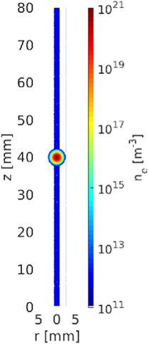
Figure 2. The simulation domain showing the electron density of the initial plasma patch (1) and of the preionization channel defined by equation (4) npre,0 = 1012 m−3. The preionized air channel is radially extended as widely as the initial electron–ion patch which is not visible because the colorbar is limited down at ne = 1011 m−3.
Download figure:
Standard image High-resolution imageWe here trace individual (super)electrons interacting with ambient air. Unlike fluid models, tracing individual (super)electrons with a particle code allows us not only to obtain streamer properties such as the electron density or electric field distribution, but also to estimate the electron energy distribution. We include electron impact ionization, elastic and inelastic scattering as well as electron attachment and bremsstrahlung. Additionally, we apply a photoionization model where photons emitted from excited nitrogen ionize oxygen molecules locally and liberate additional electrons. More details of the applied Monte Carlo model are described in [25, 55].
Since electrons ionize molecular nitrogen and oxygen, the electron number grows exponentially leading to an electron avalanche and eventually a streamer. Due to limited computer memory, we use an adaptive particle scheme [25] conserving the charge distribution as well as the electron momentum such that every simulated electron is a superelectron representing  physical electrons.
2.2. Implementation of air perturbations
In Monte Carlo particle simulations, we include the collisions of electrons with ambient air where the nitrogen and oxygen molecules are put at random positions as an implicit background. The probability Pc of a collision of an air molecule with an electron with velocity ve within the time interval Δt is  where nair is the number density of ambient air and σ the collision cross section.
Previous experiments and simulations [44, 47, 49, 56, 57] suggest that shock waves and thermal expansion by leaders and also by the small-scale discharge modes, the streamers, are capable of perturbing the vicinity of their location up to 80% of the ambient air level [47]. Within several tens of ns, the complex streamer corona simultaneously consists of a multitude of streamers [58] amongst which some reach large currents. Therefore, they develop ionization-heating instability such that they are capable of disturbing the air density experienced by other streamers. For nair, we therefore choose the ansatz

depicted in figure 3, with a global minimum on the symmetry axis (r = 0) and a global maximum on the outer boundary (r = Lr). The sinusoidal form has been computed by Marode et al [44] and is here meant to capture the minimum air density in the proximity of the channel axis driving air molecules to the exterior boundary. Otherwise, the actual form of nair is not crucial and we here limit ourselves to ξ = 0, 0.25, 0.5 since Marode et al calculated perturbation levels of 50% as an upper limit in the vicinity of a streamer. Note that the time tD of air molecules to diffuse back to uniform density is in the order of  1.8 s with Dair ≈ 2 × 10⁻⁵ m2 s−1 [59] which is much larger than the simulation time of the order of several nanoseconds allowing us to assume a stationary distribution of air molecules.
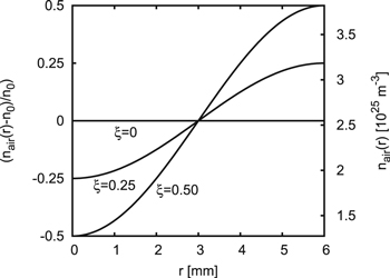
Figure 3. Air density (3) as a function of r for perturbations of 0%, 25% and 50%.
Download figure:
Standard image High-resolution image2.3. Implementation of preionization
As discussed by Babich et al [27, 42], streamers leave behind residual ionization affecting the motion of successive streamer and leader channels. The reminiscent density npre of the previous streamer channel is modeled by

where  m−3 determines the peak density and
  the width of the preionized channel. This approach is advocated, firstly because each streamer discharge has its own characteristic minimal radius depending on the streamer velocity and the ambient gas density [60], secondly because the charge and the width of the preionized channel diffuse with time [42]. In addition, Sadighi et al [61] have shown that such levels of preionization prevent streamers from branching.
After a preceding discharge, the time to readjust the electric field is in the order of some ns μs [51] which is significantly smaller than the diffusion time tD. Hence, the screening of the electric field is negligible in the current set-up which justifies to run simulations in Eamb = 1.56Ek given a fixed potential difference.
Figure 2 shows the initial electron–ion patch together with the preionized channel (λpre = λ0 and npre,0 = 1012 m−3). It illustrates how the initial electron–ion patch is embedded in the preionized channel. Note that the channel is extended radially as much as the electron–ion patch which is not visible because the colorbar is limited down at ne = 1011 m−3.
2.4. Calculation of the runaway rate
In this section we will give a brief overview how to understand and how to calculate the production rate of runaway electrons; we therefore adopt the discussion of equations (10) and (11) in [27]. The runaway rate νrun(E) at STP as a function of the electric field strength, i.e. the number of runaway electrons per unit time, used here is computed first for nitrogen through Monte Carlo simulations [62]; these Monte Carlo results are then fitted by an exponential function [27] to obtain
Although this rate is valid for nitrogen only, we here use it for air since the cross sections for the ionization and excitation of nitrogen and oxygen are almost identical except for the very small range below 20 eV and since the percentage of oxygen in air is ≈20% only.
Figure 4 shows that for fields of up to 10Ek νrun varies between approximately 10−24 and 108 s−1. For electric fields above 6Ek, it is νrun(E = 6Ek) ≈ 2.94 s−1, νrun(E = 7Ek) ≈ 990.66 s−1 and νrun(E = 8Ek) ≈ 1.28 × 10⁵ s−1; hence, the local electric field has a significant effect on the production rate of runaway electrons. The rate νrun allows us to estimate the number kRE of runaway electrons per unit length. For a negative front moving with velocity vneg, the temporal variation of the number NRE of runaway electrons obeys the differential equation dNRE(t) = kRE(t)vnegdt which is equivalent to
where the time depending number NRE of runaway electrons is [27]

where the volume integral over the simulation domain takes into account the variation of the electron density and the electric field in space and time. Note that the electron density is calculated from Monte Carlo simulations whilst  is the analytic fit (5), and that any explicit dependence on r and z is integrated out in (8). Yet, NRE depends on time t; so does the evolution of the streamer fronts. Therefore, NRE depends on the streamer length implicitly. However, because of this implicit dependency, we use the time derivative of NRE and the streamer velocity instead of the spatial derivative of NRE.

Figure 4. The runaway rate  (5) as a function of the electric field.
Download figure:
Standard image High-resolution image3. Results
3.1. Benchmarking
Babich et al [27] have already solved the fluid equations of negative streamers in preionized air without the effect of air perturbations focusing on the production of runaway electrons in a field of Eamb = 50 kV cm−1. Figure 5 compares the on-axis electron density (a) and the on-axis electric field (b) of the negative streamer front for npre,0 = 1012 m−3 computed by Babich et al and computed by MC particle simulations showing a very good agreement in the streamer channel. There is a slight deviation after 2 ns which is compensated again after 3 ns. In all considered cases, however, our results show fluctuations which do not occur in the previous results. Yet, this is not surprising since a particle code normally shows more fluctuations than a fluid code, see. e.g. [63]. At the tips, the electric field peaks as smoothly as for the fluid code. Beyond the streamer channel the electron density is larger than the electron density calculated by the fluid equations. In contrast to the fluid model, the particle Monte Carlo code allows us tracing the space-time energy distribution of each individual electron and, as a consequence, computing the spatial electron distribution more accurately. The plateau-like behavior of the electron density after 2 and 3 ns is an evidence of the polarization self-acceleration of the electron swarm moving ahead of the streamer body, as observed in experiments with nanosecond discharges at STP conditions [17, 64, 65]. Such electrons, ahead of the streamer and therefore in the channel, are continuously accelerated in the strong moving field at the streamer tip. They overtake the main bulk of electrons and are therefore disconnected from the main streamer body [66, 67]. The applied particle code is capable of capturing this effect unlike the fluid approach. Therefore, we reason that our results are more accurate than the ones obtained by the fluid model.

Figure 5. The on-axis electron density (a) and the on-axis electric field (b) as a function of z calculated from the simulations by Babich et al [27] and from our particle-in-cell (PIC) simulations for a preionization level of 1012 m−3 without any air perturbation.
Download figure:
Standard image High-resolution image3.2. Streamer evolution in uniform, preionized air
We here commence our study of the streamer evolution in preionized air only, similar to the set-up discussed in [27].
Figure 6 compares the electron density and the electric field in non-ionized air with the electron density and the electric field in preionized air with  m−3. After 1.62 ns the streamer length and the electric field are equally large irrespective of npre,0. After 2.84 ns, however, the streamer in preionized air overtakes the streamer in non-ionized air and the field at the streamer tips is slightly more enhanced. In addition the density of the preionized channel has reached values of above 1015 m−3 distributed uniformly beyond the streamer tips which is not the case in the absence of preionization. Finally, after 3.44 ns, the streamer channel in preionized air has completely grown into the preionized channel (within the simulation domain) and has proceeded approximately twice as much as the streamer in non-ionized air.
Figures 7(a) and (b) show the streamer velocities of the negative and positive fronts in non-perturbed air. It shows that initially streamers move comparably fast for different levels of preionization. After a few ns, however, streamers in the highest level of preionization, here npre,0 = 1013 m−3, accelerate more effectively than streamers in non-ionized air, followed by streamers in air with descending order of preionization.

Figure 6. The electron density (top) and the electric field (bottom) in non-ionized air (left half of each panel) and in preionized air with npre,0 = 1012 m−3 (right half) after different time steps.
Download figure:
Standard image High-resolution image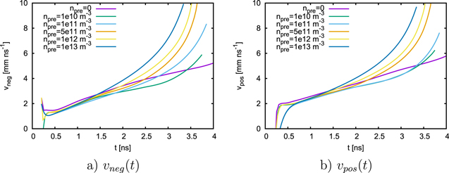
Figure 7. The velocities of the negative (a) and positive (b) streamer front in uniform air for different levels of preionization as a function of time.
Download figure:
Standard image High-resolution imageThe different acceleration of streamers in non-ionized and in preionized air is a result of the space-charge induced electric field. In the early stages of the streamer development there is no significant contribution of the preionized air channel. However, after several time steps depending on  , the streamers grow into the preionized channel and hence the electric field at the tips energizes the channel electrons in the vicinity of the streamer head. These channel electrons subsequently gain enough energy to ionize molecular nitrogen and oxygen and create additional space charge in the proximity of the streamer head; thus, the electric field and the velocities of streamers in highly ionized air exceed the field and velocities of streamers in less ionized air.
3.3. Runaway electron production in uniform and preionized air
Let us now turn to the production properties of runaway electrons from streamers in preionized air as they might occur after the reconnection of the space stem with a stepping leader. Note that the runaway threshold energy depends on the electric field [13]: for an electric field of 1.56Ek sea-level equivalent the runaway threshold energy amounts to 5 keV; for a field of 0.5Ek, it amounts to approx. 21 keV. These are, however, the runaway thresholds in a homogeneous electric field; in concrete streamer simulations, the field at the tip actually grows to field strengths larger than 0.5Ek or 1.56Ek and therefore, the runaway threshold energy becomes smaller than 5 or 21 keV.
Table 1 shows that for Eamb = 1.56Ek  , the maximum of kRE(t) over time, is smallest in non-ionized air and increases until npre,0 = 1011 m−3 since the maximum electric field at the streamer tips increases with the level of preionization until npre,0 = 1011 m−3. This increase results from the more enhanced electric field at the streamer tips for larger preionization. In turn, above npre,0 = 1011 m−3, the high electron density in the vicinity of the streamer front screens the electric field at the tips and thus limits the maximum field strength and the maximum number of runaway electrons. Table 1 also compares our results with the runaway rate kRE,Babich by Babich et al [27] which is defined in a different manner:
This definition includes the number of runaway electrons produced between the time steps when the front has reached zf = 2.9 and 3.0 cm, to the end of their simulations. Since previous simulations and our simulations behave slightly differently, we compare kRE,Babich with  calculated from our simulations. kRE,Babich reaches its maximum for npre,0 = 1012 m−3 and amounts to 2 × 10⁹ m−1 whereas
  in our simulations reaches its maximum for npre,0 = 1011 m−3 and amounts to ≈2.12 × 10⁹ m−1. Thus, we find a good agreement between these two maxima within one order of magnitude of npre,0. Additionally, we here confirm the findings by Babich et al [27] that the number of runaway electrons is enhanced if streamers move in preionized air. We also observe both with Monte Carlo or fluid simulations that the runaway rate per unit length decreases for smaller and larger preionization densities npre,0. Since, we observe the same tendency for the two different models, we reason that the one order of magnitude difference is due to the different definitions of (6) and (9): (6) gives the production rate at each moment of time during the simulation, whereas (9) determines the production rate only at the final stage of the streamer development.
Table 1.
The maximum number of produced runaway electrons per unit length,  , the maximum electron energy
  , and the maximum electric field maxt E as a function of npre,0. For comparison, we also show kRE,Babich (9).
| npre,0 (m−3) |
 (m−1) (m−1) |
kRE,Babich (m−1) |
 (eV) (eV) |
 (MV m−1) (MV m−1) |
|---|---|---|---|---|
| 0 | 2.92 × 10³ | — | 252 | 22.43 |
| 1010 | 1.88 × 10⁸ | 2 × 10⁴ | 358 | 31.05 |
| 1011 | 2.12 × 10⁹ | 5 × 10⁷ | 16 883 | 33.08 |
| 5 × 10¹¹ | 1.68 × 10⁶ | — | 13 579 | 23.04 |
| 1012 | 8.06 × 10⁶ | 2 × 10⁹ | 10 160 | 23.03 |
| 1013 | 7.48 × 10⁶ | 9 × 10⁸ | 1367 | 22.98 |
Table 1 also shows that similarly to the maximum runaway rate, the maximum electron energy increases until npre,0 ≈ 1011 m−3 and decreases for higher levels of preionization. Whereas the maximum electron energy in non-ionized air is approx. 250 eV, the maximum electron energy for npre,0 = 1011 m−3 amounts to approximately 17 keV and decreases to approximately 1 keV for npre,0 = 1013 m−3 which is sufficiently high for electrons to overcome friction and initiate a relativistic runaway electron avalanche [22].
3.4. The additional effect of air perturbations on runaway electrons
After we have discussed the sole effect of preionization, we now focus on the effect of air perturbations coinciding with the preionization of air as it might occur in the complex streamer corona in the proximity of lightning leaders.
As we have shown in [50], streamers move faster in perturbed air with  similarly we have discussed in section 3.2 that streamers move faster in preionized air with npre,0 = 1011–1015 m−3. As a result from the combination of both effects, we have observed in our simulations that streamers move fastest in perturbed and preionized air with
  and npre,0 = 1011–1015.
Figure 8(a) shows  , as a function of npre,0 for different levels of air perturbation. It shows that in non-ionized air the number of runaway electrons increases with the level of air perturbation. As for the streamer velocities, the increase of the number of runaway electrons results from the enhanced reduced electric field in the vicinity of the symmetry axis (see [51]). If the effects of air perturbation and of preionization are combined, we observe a reversed trend compared to in uniform air because of the significant growth of the electron density in the vicinity of the streamer head in perturbed air even for small levels of preionization. Instead of increasing, the number of runaway electrons in perturbed air decreases with the preionization level. For npre,0 ≈ 1010 m−3,
  is approximately 109 m−1 for all levels air perturbation; for larger npre,0, the number of runaway electrons in non-perturbed air exceeds that in perturbed air. Although the runaway rate decreases for npre,0 = 1013 m−3,
  is some orders of magnitude higher in perturbed air than in uniform and non-ionized air. Ultimately, the number of runaway electrons is highest for ξ = 0.5 in non-ionized air and for npre,0 ≈ 1011 m−3 in uniform air with ξ = 0.
Figure 8(b) compares the maximum electron energy in perturbed air with that in non-perturbed air for npre,0. For a perturbation level of ξ = 0.25, the maximum electron energy varies from approximately 4–13 keV for npre,0 < 1011 m−3 which is one order of magnitude larger than in uniform air and high enough to start runaway electron avalanches. Above  m−3, the maximum electron energy varies between approximately 13 and 1 keV which is comparable to
  in non-perturbed air.
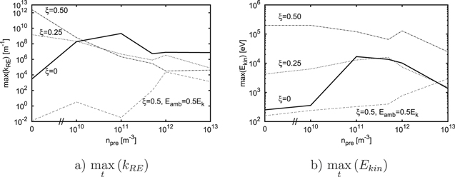
Figure 8. (a) The maximum number of runaway electrons per unit length,  , as a function of npre,0 for λpre = λ0 and different levels ξ of air perturbation. (b) The maximum electron energy
  for λpre = λ0 and different ξ. If not denoted otherwise, the ambient field here amounts to 1.56Ek.
Download figure:
Standard image High-resolution imageFor ξ = 0.5, the maximum electron energy is highest and varies between 200 and 25 keV which is significant enough to trigger a relativistic avalanche for any level of preionization. In contrast to ξ = 0 and ξ = 0.25, there is not a distinct maximum between npre,0 = 1011 and 1012 m−3.
Conclusively, we identify three regimes: (i) for air perturbations below  and for preionization levels below npre,0 = 1011 m−3, the air perturbation determines the maximum electron energy whereas (ii) for
  m−3 the influence of the air perturbation is negligible and the maximum electron energy is determined by npre,0; (iii) for air perturbations as large as ξ = 0.5, the maximum electron energy is mainly determined by the air perturbation with minor effect of the preionization level.
3.5. The streamer velocity and the production of runaway electrons in subbreakdown fields
So far, we have discussed the streamer velocity and the effect of preionizing and perturbing air on the production of runaway electrons in an ambient field of 1.56Ek. However, the multitude of streamers adjacent to leader stepping also effects the electric field distribution in the corona. As an example, we therefore now turn to the production of runaway electrons in a subbreakdown field of 0.5Ek. Note that the value of this field refers to the electric field strengths in uniform air. Thus, Eamb = 0.5Ek means 0.5 times the breakdown field in uniform air with density n0. Hence, if ξ = 0.5, a field of 0.5Ek is the same field strength as the breakdown field strength in unperturbed air for r = 0 decreasing for r > 0. For ξ < 0.5 the electric field strength would be below the breakdown field value in the whole simulation domain and therefore we only consider ξ = 0.5 and Eamb = 0.5Ek.
For this particular set-up, figure 9 shows the streamer velocities at the negative (a) and positive (b) front as a function of time for different levels of preionization. We observe a similar dependency on preionization as in Eamb = 1.56Ek. For time steps  ns, the preionization effect is negligible; for larger time steps, streamers accelerate more efficiently when wave fronts grow into preionized air with larger npre,0. Such waves create more space charges, thus induce higher self-consistent electric fields and lead to more efficient streamer acceleration.
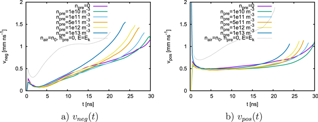
Figure 9. The streamer velocities of the negative (a) and positive (b) front as a function of time for ξ = 0.5, Eamb = 0.5Ek and different levels npre,0 of preionization. For comparison, the dotted line shows the streamer velocities in non-ionized and uniform air in an ambient field of Ek.
Download figure:
Standard image High-resolution imageFor comparison, the dotted line shows the front velocity in non-perturbed air with  ,
,  and Eamb = Ek. This comparison reveals that the streamer fronts move significantly slower for ξ = 0.5 and Eamb = 0.5Ek than for ξ = 0 and Eamb = Ek because of the non-uniformity of the air perturbation. Only at the symmetry axis where nair = 0.5n0 is the reduced electric field E/nair comparably large as Ek/n0 in non-perturbed air. Since the reduced electric field decreases with r, the streamer motion is damped for r > 0, and the streamers move slower in perturbed air.
This effect of air perturbations on the reduced electric field is visualized in figure 10. It shows the electron density for ξ = 0 and Eamb = Ek and for ξ = 0.5 and Eamb = 0.5Ek. It shows that after 5 ns the streamer in uniform air moves faster and is thicker and more diffuse than in perturbed air. The reason for this is again that the reduced electric field in perturbed air decreases as a function of r and thus generates a quenching effect on the streamer in Eamb = 0.5Ek.
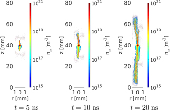
Figure 10. The electron density (first row) in non-ionized air with Eamb = Ek and ξ = 0 (left half of each panel) and with Eamb = 0.5Ek and ξ = 0.5 (right half).
Download figure:
Standard image High-resolution imagePanels (a) and (b) of figure 8 compare the maximum runaway production rate and the maximum electron energy for ξ = 0.5 and Eamb = 0.5Ek with the rates and energies of electrons from streamers in Eamb = 1.56Ek. There are two effects contributing to the production runaway electrons in subbreakdown fields in our simulations: firstly, the air perturbation level ξ = 0.5 ensures that for r = 0 the reduced electric field is effectively as large as the breakdown field in unperturbed air; secondly, as we have seen in section 3.3, levels of preionization between 1010 and 1013 m−3 enhance the production of runaway electrons. For  m−3 the runaway rates and the maximum electron energy are smaller than in uniform air. For
  m−3, however,
  becomes comparable to the one in uniform air in 1.56Ek. The maximum electron energy in this set-up increases with npre,0 and reaches approximately 3 keV which allows the formation of runaway electron avalanches in subbreakdown fields.
3.6. Variation of the channel radius
Whereas the previous results were obtained for λpre = λ0, we now discuss how the streamer velocities and the number of runaway electrons change for λpre = 0.5λ0 and for λpre = 1.5λ0.
Note that the absence of any preionization is equivalent to  and the presence of uniform background ionization in the complete simulation domain is equivalent to
  . In our simulations we have observed that in non-perturbed air, both the positive and the negative streamer front move faster for small channel radii and slower for large channel radii. In contrast, for ξ = 0.5, there is no significant difference between λpre = 0.5λ0 and λpre = λ0; yet, for a wide channel with λpre = 1.5λ0 the streamer moves slower than in small channels. This is consistent with modeling results of streamer heads under different levels of uniform background ionization [43] which have shown that streamers move faster in the absence of any background ionization than in the presence of uniform background ionization.
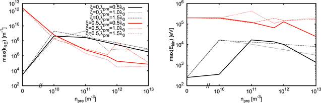
Figure 11 compares  and
and  for different npre,0 and λpre. Note that there is no channel for npre,0 = 0, thus we only use the values for npre,0 = 0 as comparison. These panels show that for
  , the maximum generation rate of runaway electrons is slightly higher than in preionized air with λpre = λ0. Still, the overall trend is the same regardless of λpre. In non-perturbed air, the maximum generation rate
  of runaway electrons reaches its maximum for
  at npre,0 = 1010 m−3, and decreases for larger preionization levels. In perturbed air,
  is maximal for npre,0 = 0 and decreases for npre,0 > 0.
Figure 11. (a) The maximum number of runaway electrons per unit length  and (b) the maximum electron energy
  for different channel radii λpre as a function of npre,0.
Download figure:
Standard image High-resolution image
4. Discussion and conclusion
We have discussed how the preionization  , the width λpre of the preionized channel and the air perturbation level ξ adjacent to leader stepping influence the streamer velocities, the maximum electron energy and production rate of runaway electrons in streamer discharges and thus affect the production rate of x-ray bursts after the leader stepping.
In all considered cases, above and below the classical breakdown field, we have seen that increasing both the level of preionization and of air perturbation raises the streamer velocities at the positive and negative fronts. When increasing the amount of preionization in uniform air, initially there is no difference in the streamer velocities before streamers in highly ionized channels begin to accelerate more prominently than in less ionized air. This is due to the enhanced electric field induced by the elevated amount of space charges produced by streamers growing into channels with high preionization. However, the streamer velocity is primarily affected by air perturbations since the electron motion and hence the streamer development are determined by the reduced electric field E/nair. In addition, the width of the preionized channel has a marginal effect on the streamer velocity: Thinner channels accelerate more significantly than thicker channels.
Our simulations have shown that in the absence of any air perturbations, the generation of runaway electrons increases with npre,0 up to npre,0 ≈ 1011 m−3 and decreases for higher preionization since the additional space charges then shield the electric field reducing the electron acceleration and thus the production of runaway electrons.
Enabling air perturbations in non-ionized air increases the runaway electron production rate per unit length which is consistent to previous simulations [51]. However, increasing npre,0 decreases the runaway electron production rate in contrast to increasing npre,0 in uniform air; yet these rates are larger than in non-ionized and uniform air.
Preionization and air perturbations also allow for the production of runaway electrons below the classical breakdown field. In a field of Eamb = 0.5Ek, 50% air perturbation and preionization levels larger than 1012 m−3, the production rate of runaway electrons lies within one order of magnitude of the production rate of runaway electrons in 1.56Ek.
Together with these runaway production rates, the maximum electron energies vary from some keV in non-perturbed and ionized air up to hundreds of keV in perturbed air. Under these circumstances, the electron energies are sufficiently high to initiate secondary relativistic runaway electron avalanches.
For the cases considered, table 2 summarizes the production rate per unit time defined as NRE(tmax)/tmax where NRE(tmax) is the total number of runaway electrons and tmax the time step at the end of the simulation. In non-perturbed and preionized air, this rate varies between ≈1014 and 1012 runaway electrons per second. In perturbed air with ξ = 0.25 and ξ = 0.5 and npre,0 < 1011 m−3 these rates vary between 1012 and 1017 s−1. Measurements by Schaal et al [68] have revealed that the rate of energetic electrons producing x-rays adjacent to lightning discharges varies between 1012 and 1017 s−1 which can be explained by the scenarios discussed in the present study.
Table 2. The rate of runaway electrons per unit time (s−1) for different levels of preionization and air perturbation.
| ξ | |||
|---|---|---|---|
| npre,0 (m−3) | 0 | 0.25 | 0.5 |
| 0 | 1.56 × 10⁸ | 6.33 × 10¹³ | 3.32 × 10¹⁷ |
| 1010 | 1.55 × 10¹⁴ | 2.37 × 10¹⁴ | 2.98 × 10¹⁴ |
| 1011 | 6.61 × 10¹⁴ | 2.24 × 10¹² | 1.04 × 10¹⁴ |
| 5 × 10¹¹ | 1.72 × 10¹³ | 5.96 × 10¹¹ | 5.96 × 10¹¹ |
| 1012 | 7.03 × 10¹² | 1.52 × 10¹² | 1.04 × 10¹¹ |
| 1013 | 5.3097 × 10¹² | 5.46 × 10¹⁰ | 3.87 × 10¹⁰ |
Celestin and Pasko [26] estimate that the streamer corona in the vicinity of a leader tip consists of approximately 106 streamers. Hence, applying the runaway rates calculated for one streamer, we estimate the maximum rate of energetic electrons in preionized or perturbed air to lie approximately between 1018 and 1023 s−1 for the whole streamer zone. Note, however, that such a multitude of streamers influences the properties of each individual streamer through streamer collisions [35–37, 69] as well as through ionizing [42] or perturbing ambient air [44, 47]. Hence, the runaway rate of 1018–1023 s−1 can only be an upper limit of the real value of energetic electrons emitted by the whole streamer zone.
Yet, our findings are in agreement with observations. Thus, the amount of preionization and air perturbation established by preceding streamers adjacent to lightning leaders is sufficient to create energetic electrons, significantly multitudinous to contribute to the emission of energetic photon bursts in the proximity of lightning leaders.
Acknowledgments
This project has received funding from the European Unions Horizon 2020 research and innovation programme under the Marie Sklodowska-Curie grant agreement 722337. The simulations have been performed on the Bridges at PSC and the Comet at SDSC which are supported by the NSF.