
Abstract
In high power impulse magnetron sputtering (HiPIMS) bright plasma spots are observed during the discharge pulses that rotate with velocities in the order of 10 km s−1 in front of the target surface. It has proven very difficult to perform any quantitative measurements on these so-called spokes, which emerge stochastically during the build-up of each plasma pulse. In this paper, we propose a new time shift averaging method to perform measurements integrating over many discharge pulses, but without phase averaging of the spoke location, thus preserving the information of the spoke structure. This method is then applied to perform Langmuir probe measurements, employing magnetized probe theory to determine the plasma parameters inside the magnetic trap region of the discharge. Spokes are found to have a higher plasma density, electron temperature and plasma potential than the surrounding plasma. The electron density slowly rises at the leading edge of the spoke to a maximum value of about 1 × 10²⁰ m−3 and then drops sharply at the trailing edge to 4 × 10¹⁹ m−3. The electron temperature rises from 2.1 eV outside the spoke to 3.4 eV at the trailing end of the spoke. A reversal of the plasma potential from about −7 V outside the spoke to values just above 0 V in a spoke is observed, as has been proposed in the literature.
Export citation and abstract BibTeX RIS

Original content from this work may be used under the terms of the Creative Commons Attribution 3.0 licence. Any further distribution of this work must maintain attribution to the author(s) and the title of the work, journal citation and DOI.
1. Introduction
High power impulse magnetron sputtering (HiPIMS) is a recent variant of magnetron sputtering where high voltage pulses are applied to a magnetron instead of a continuous voltage. The high voltage creates a dense plasma which can be close to full ionization [1]. The resulting high ion fluxes onto the substrate lead then to coatings of superior quality compared to those deposited with traditional direct current magnetron sputtering (DCMS) [2, 3]. However, this improvement in coating quality is usually accompanied by a reduction in deposition rate [4, 5].
HiPIMS discharges are pulsed at repetition frequencies between a few Hz to a few kHz and pulse lengths between a few and a few hundred microseconds. The peak discharge power density, normalized to the cathode surface, is usually in the order of 1 kW cm−2. Above a circular target, the plasma forms a torus shape created by the magnetic field configuration. Below the plasma torus intense sputtering occurs and forms the so-called racetrack on the target.
The plasma torus is not homogeneous but instead exhibits one or more spots of enhanced emission intensity, which rotate with about 10 km s−1 in E × B direction [6]. These bright spots have been coined spokes, in resemblance to similar features found in Hall thrusters [7]. Spokes have been investigated both in terms of their properties like velocity [7–9], shape [6, 7, 9, 10] and mode number [6, 7, 9] and also in terms of their influence on ion transport [11–16]. All these experiments base their analysis on time averaged data or on time-resolved data that was recorded outside of the spokes.
In contrast, measurements of internal properties of the spokes are sparse, due to severe experimental difficulties: (i) on the one hand, spokes are located very close to the target surface inside the magnetic trap [11, 17] which makes probe measurements very invasive. Additionally, probe measurements inside magnetic fields are challenging and require a detailed analysis with respect to the magnetic field configuration around the probe tip [18]; (ii) on the other hand, spokes are inherently stochastic in their nature. Even though it is possible to assign an average mode number and velocity to the spokes for a given set of discharge parameters, the precise spoke properties and their timing will change from one HiPIMS pulse to the next [9, 16]. Thus, simply averaging signals obtained over many discharge pulses yields no detailed information on an individual spoke since all fluctuations caused by the spokes will simply average out. Therefore, all measurements of spoke properties are preformed in single-shot manner only up to now and more demanding diagnostic methods that require longer acquisition times are currently not applicable.
Given these two problems, only few attempts have been made to determine plasma parameters of individual spokes. Poolcharuansin et al [19] and later Klein et al [20], used a segmented cathode to observe spoke induced target current fluctuations onto those segments. Depending on the discharge parameters, they found an up to 60 % higher current when a spoke was present above the cathode segment. Similarly, Hecimovic et al used probes embedded in the target surface, instead of segments [21]. This enabled the authors to calculate a local current density and from this the plasma density at the sheath edge. They found the plasma density to fluctuate between 5 × 10¹⁹ m−3 and 9 × 10¹⁹ m−3. However, to calculate the density from the current, the authors had to assume a constant electron temperature and that the ions arrive at the sheath edge with the Bohm speed, which is only a rough estimate in HiPIMS plasmas [22, 23].
Panjan and Anders used a two probe setup containing a heated emissive probe and a cold floating probe to investigate the plasma potential and floating potential of spokes in a DCMS discharge [24]. The authors achieved discharge conditions under which the spokes were highly stable and reproducible, making synchronization and averaging of the data unnecessary. The authors found the plasma potential to fluctuate between −80 V and −10 V when the probe was positioned 2.5 mm above the racetrack of the 3'' niobium target. The fluctuations became weaker with increasing distance to the target surface. The authors also used the difference between plasma and floating potentials to investigate the electron energy, which was shown to increase with the plasma potential inside the spoke.
Lockwood Estrin et al used a triple probe to measure plasma parameter fluctuations caused by the spokes [25]. They found the plasma density to fluctuate between n = 1 × 10¹⁹ m−3 and n = 2 × 10¹⁹ m−3 and the electron temperature between  eV and
  . The plasma potential Vp measured by the authors was always positive, fluctuating between 0 V and 8 V. However, in order to reduce disturbances of the discharge and to avoid problems caused by magnetized electrons, the measurement position was close to the magnetic null, 15 mm above a 3'' target. Consequently, no distance variation was performed to explore the internal spoke structure.
In this work, we use a conventional Langmuir probe to measure plasma parameters of HiPIMS spokes using aluminium as the target material. As a Langmuir probe is much smaller than a triple probe, we can get closer to the target surface and penetrate into the spoke structure without critically disturbing the discharge. We present a time shifting method to average over many discharge pulses without loosing the spoke information in the process. Thereby, an average spoke is created. The resulting I–V curves are evaluated explicitly including magnetized electrons in the calculations. In this way, we obtain the plasma density, electron temperature and plasma potential time resolved for an average spoke under our discharge conditions.
2. Experimental setup
2.1. HiPIMS setup
Figure 1(a) shows the experimental setup, including the probe circuitry and the optical setup. The vacuum chamber had a base pressure of 4 × 10⁻⁶ Pa. 40 sccm of argon was continuously flowing into the chamber during discharge operation resulting in a working gas pressure of 0.5 Pa. The discharge was ignited using a magnetron suitable for circular 2'' targets. For this study, we used an aluminium target with a thickness of 3 mm.
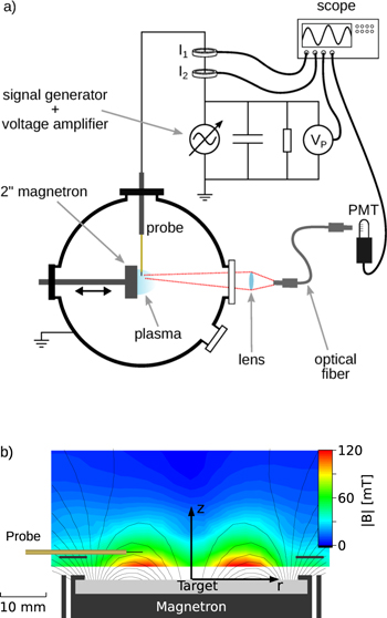
Figure 1. (a) The experimental setup including the probe circuitry and the optical setup for the photo multiplier (PMT). (b) Cross section of the magnetic trap region above the magnetron showing the measured magnetic field strength on the color map and the simulated magnetic field lines. The indicated probe location is for  . Drawing is true to scale.
Download figure:
Standard image High-resolution imageThe power supply (TRUMPF Hüttinger TruPlasma Highpulse 4002) was connected to the target with an additional inductance to limit the current rise during discharge operation. Current and voltage were continuously measured between inductance and magnetron using current and voltage probes (Tektronix TCP A400, Tektronix P6015A). The probe signals were recorded by a Tektronix TPS 2024 oscilloscope (not shown in figure 1). The electrical setup has been described in more detail in [26].
The discharge pulses were set to a length of 100 μs with a repetition rate of 30 Hz. The discharge voltage was 670 V before breakdown and around 570 V after breakdown during the pulse. The current onset was at about 18 μs. A maximum current of 40 A or a target current density of 2 A cm−2 was reached, respectively, at the end of the pulse (compare figure 6). The peak target power density during the pulse was thus 1.15 kW cm−2.
Figure 1(b) shows a cross section of the magnetic trap region above the target. As the figure indicates we use a cylindrical coordinate system with z as the target normal coordinate, r in the radial direction and ϕ in azimuthal direction (not shown in the figure).
2.2. Optical reference signal
The main idea of the experiment is to monitor the movement of the spokes with a photo multiplier used to identify the proper location of an individual spoke. With this information, the current acquired with the Langmuir probe for a single plasma pulse is shifted in time, so that the averaging over many plasma pulses renders a complete set of Langmuir I–V curves of a single spoke.
The photo multiplier (PMT, Hamamatsu R928) was used to provide the reference signal for the probe measurements. An optical fibre (100 μm diameter), combined with a biconvex (f = 160 mm) lens was used to limit the field of view to a 1 mm diameter dot on the target. The field of view was adjusted to collect the light emitted right next to the probe tip, shifted only by about 150 μm in E × B direction. The PMT was terminated with 500 Ω and connected to an oscilloscope (Teledyne LeCroy waverunner 8404M-MS).
2.3. Langmuir probe
The probe was inserted from the side of the magnetron, as shown in figures 1(a) and (b). The self-built probe consist of a 125 μm thick tungsten wire, that is protected by two ceramic tubes (diameters: 0.6 mm and 1.2 mm). The smaller of the two tubes is slightly retracted so that a gap between probe and outer tube is created. This prevents electrical contact between the wire and the outer shielding, which might occur once enough aluminium has been deposited on the ceramic to create a conducting coating. The 3.5 mm probe tip was positioned above the middle of the racetrack. The distance between probe tip and target surface was varied by moving the magnetron. Three distances were chosen in the study:  , and
, and  . The probe position for
  is shown in figure 1(b). The figure also shows the magnetic field lines simulated with FEMM and the measured magnetic field strength as a color map [27].
The probe voltage was provided by a signal generator (Tektronix AFG 3102) combined with a voltage amplifier (KEPCO BOP 100-2M). The voltage was slowly swept from −80 V to 8 V using a ramp signal with a frequency of 0.9 Hz. In this way, the probe voltage was nearly constant during a single discharge pulse. Afterwards, a complete probe current–voltage curve (I–V curve) for each point in time, is assembled from measurements over many subsequent pulses as it is usually done in Langmuir probe measurements in HiPIMS [28, 29]. The voltage was measured using a capacitive voltage probe (Teledyne LeCroy PP022).
A capacitor (20 μF) and a resistor (1 kΩ) were connected in parallel to the probe power supply, as indicated in figure 1(a). This circuitry acted as a low pass filter to keep the voltage constant during the pulse, as the voltage amplifier alone was not able to react fast enough to the current fluctuations caused by the spokes. Some oscillations with very precise frequency of 8.3 MHz were observed in the probe current. These were removed by filtering in the post-processing of the data.
It is a common problem with probe measurements to measure both the large electron current and the much smaller ion saturation current with satisfactory precision. To overcome this problem we used two Pearson 2877 current probes (I1 and I2 in figure 1(a)) to measure the probe current. The current probes were connected to the oscilloscope (Teledyne LeCroy waverunner 8404M-MS). One of the oscilloscope channels was set to digitize small currents between −50 mA and 30 mA, whereas higher currents would saturate this channel. The higher currents were measured instead using the second current monitor on a different channel set to be less sensitive. Both current time traces were saved for each discharge pulse and the appropriate current readout was selected in post-processing. The Pearson 2877 current probes employed here were found to exhibit a slight drool (dropout of slow signals) at the end of the discharge pulse as was deduced from a comparison with an alternative current probe (ELDITEST CP6550). This drool may cause slightly attenuated signals and thus an apparently lower plasma density. This difference was less than 10 % and is much smaller compared to other sources of errors as will be discussed below.
The probe was found to slightly disturb the discharge when operated at the closest position ( ). The mere presence of the probe without any voltage applied (floating) caused the plasma to ignite slightly later, at
  instead of
  . The maximum current that was reached was also reduced by about 1 A, or 2.5 %. A stronger change was observed, however, when drawing electron saturation current leading to a delay in the current onset up to 4 μs and a reduction of the maximum current by up to 4 A, or 10 %. This influence of the probe on the plasma does not affect our analysis, because any data on the electron current close to saturation are also not reliable, as explained in the appendix.
2.4. Data acquisition
The signals of both the PMT reference and the probe were recorded by an oscilloscope (Teledyne LeCroy waverunner 8404M-MS) that was triggered on the discharge pulse by the power supply and was set to acquire time traces for all four channels (probe voltage, two times probe current, PMT) as fast as possible and then save them to disk for each acquisition. The sampling rate was adjusted to 2.5 GS s−1. Because of the time needed to write the acquired data to the hard drive, the oscilloscope was only able to acquire the data with a frequency of about 16 Hz. Consequently, only every second discharge pulse could be measured. Data from 50 000 pulses were saved for each of the three investigated positions, leading to measurement times of about one hour and about 90 GB of data. During the time, the discharge was found to be very stable. Only a very slight drift in peak current by less than 1 A could be observed.
3. Signal processing and probe data interpretation
In order to obtain a probe I–V curve of a HiPIMS plasma, the probe voltage is slowly swept and the current is measured over many consecutive discharge pulses. The probe current–voltage curve is then reassembled in post processing. This step scan approach will usually average out the influence of spokes, because of the pulse to pulse differences in the time at which spokes occur.
Here, we use the photo multiplier as a reference to synchronize the probe diagnostic to the spoke appearance. Signals are first shifted in time and only then averaged in order to create an average spoke. This time shift averaging method is similar to cross-correlation spectroscopy [30] of short pulsed plasmas with stochastic plasma ignition or can be described as a time shifted variant of the step scan method as it is used in infrared spectroscopy.
3.1. Signal processing under time shift averaging
Figure 2 shows an illustration of time shift averaging approach. Figure 2(a) shows three PMT time traces, obtained from three consecutive discharge pulses (the signals are offset by 0.5 V for readability). The signals show distinct peaks corresponding to bright spoke structures moving past the PMT field of view. Averaging over the three signals in figure 2(a) would render the peaks much smaller, averaging over very many of these time traces would remove the spoke peaks entirely. Instead, we first define a reference time, in this case 95 μs. Next, we employ a peak finding algorithm to detect the spoke peaks and then shift the signals in time, so that, for each time trace, a spoke peak is located at the reference time of 95 μs: here, the first signal is shifted by 0.5 μs to the left, the second signal by 0.6 μs to the right, and the third signal by 2 μs also to the right. An average over these shifted signals renders now a sharp average spoke at the reference time. All other spokes will be attenuated because the spoke frequency exhibits a residual jitter.
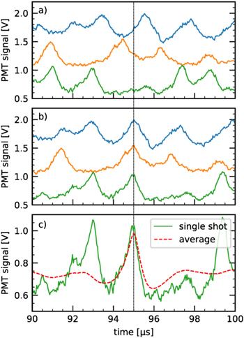
Figure 2. Illustration of time shift averaging of PMT signals. (a) Three PMT signals showing distinct spokes. Signals are offset by 0.5 V. (b) Signals from a, shifted in time so that for each signal a peak is present at 95 μs. (c) Comparison of time shift averaged spoke signal with single shot signal.
Download figure:
Standard image High-resolution imageThe peak detection is performed using the 'find_peaks' function of the scipy.signal package (version 1.2.1) for the Python programming language. The function has the optional feature to only detect peaks above a certain prominence, which is defined as the difference between the local maximum and the next minimum on either side of the peak. This feature is used to only detect strong peaks corresponding to spokes and not the smaller fluctuations caused by instrument noise (visible in figure 2).
Figure 2(c) shows an average spoke at 95 μs that is created by the time shift average of PMT traces from 500 discharge pulses (dashed line). As a comparison, the figure also shows a single PMT trace again. The average spoke is slightly attenuated compared to the single-shot measurement and slightly less asymmetric. However, the general shape and amplitude of the fluctuation is preserved. Furthermore, this average spoke signal is highly reproducible for a given set of discharge parameters and thus allows the comparison of measurements with different diagnostics using the PMT signals as a reference. For example, in our case, the PMT signals and the probe currents are recorded simultaneously by the same oscilloscope. Each current signal is shifted by the same amount as the PMT signal and can thus be averaged afterwards without losing the spoke information. In this way, assembling the data collected for different probe voltages yield a proper Langmuir I–V curve of a single average spoke.
To understand the signal created by this time shift averaging, it is instructive to discuss the PMT trace itself. Figure 3 shows the PMT signal created by time shift averaging over 500 discharge pulses. The lower part of the figure shows a zoom on the end of the discharge pulse. The strongest peak (marked 1 in the figure) is located at the reference time of 95 μs, as expected. The second largest peak (marked 1') is located at about 85 μs. Between those two large peaks, three smaller peaks can be identified, marked 2, 3 and 4. We explain this pattern as follows: peak 1 is the main spoke that constitutes our reference signal that is used as basis for the time shift averaging. Peak 1' is the same spoke from a previous revolution of the spoke pattern. Peaks 2, 3 and 4 are other spokes that are simultaneously present in the discharge. Peak 1' is more pronounced, because the spoke rotation velocity is rather stable and the peak of the previous revolution of the spoke pattern is well preserved under averaging. However, spoke patterns with higher mode numbers such as 4 in this case are less stable, and are fluctuating between mode number 2 and mode number 5 at random. Thus, all peaks corresponding to other spoke patterns are strongly attenuated, resulting in the smaller peaks 2, 3 and 4. The whole pattern is repeated for the previous revolution of the spoke pattern earlier in time (peak 1'–4').

Figure 3. PMT signal obtained by time shift averaging over 500 discharge pulses.
Download figure:
Standard image High-resolution imageBased on this interpretation, it is directly possible to determine the average spoke mode number and the spoke velocity. For the spoke mode number we find 4, as already mentioned. The spoke velocity can be calculated from the shift between peak 1 and peak 1' to  = 8.2 km s−1 using the racetrack radius of
  . These values were confirmed by camera measurements and are in line with previous observations [8].
3.2. Algorithm for I–V curve reconstruction
To reconstruct probe I–V curves for every point in time during the discharge pulse, the data acquired over 50 000 discharge pulses were processed as follows:
- (i)First, the time resolution of the acquired data was reduced from 0.4 ns to 16 ns by averaging in order to reduce both file size and noise. A FFT (fast Fourier transform) notch filter was applied to the current signals in order to remove the spurious oscillations at 8.3 MHz.
- (ii)Next, the current and PMT data was sorted into 450 voltage bins from −80 V to 8 V following the probe voltage ramp with a bin size of 0.2 V.
- (iii)The signals in each bin were time shift averaged to
 . To this end, each PMT signal was shifted in time as described in section 3.1. To each PMT signal, the simultaneously measured probe current signal, belonging to the same discharge pulse, was shifted by the same amount. Subsequently, all shifted current signals in each bin were averaged.
 - (iv)The time resolution was further reduced to 80 ns to further reduce the noise.

This algorithm yields about 1500 I–V curves at different times during and after the HiPIMS pulse.
3.3. Langmuir probe data interpretation
The usual way to determine plasma parameters (Te, n, Vp) from a Langmuir I–V curve makes use of the Druyvesteyn formula connecting the second derivative of the electron current to the electron energy probability function (EEPF) [31]. From the EEPF, plasma parameters can be deduced. However, in our case, the electron current onto the probe is strongly reduced by the magnetic field and the relationship between EEPF and electron current is more complicated. Therefore, we instead use analytical expressions for the ion and electron currents contributing to the Langmuir probe current and fit these to the measurement, as described in the following:
For the ion current, we use the calculations of Bernstein, Rabinowitz and Laframboise (BRL) in the parameterization of Chen [32–34]. For the ion mass we use  , the rounded down mean value of the mass of argon and aluminium. The influence of double charged ions is neglected. For the electron current, the strong magnetic field at the position of our measurement (about 60 mT) has to be taken into account, as the magnetic confinement of electrons is expected to strongly reduce the electron current onto the probe. According to the probe theory for magnetized electrons developed by Arslanbekov et al and extended by Popov et al the electron current Ie is [35, 36]:
for electrons with an isotropic energy probability function (EEPF) of f0. W is the energy of an electron inside the probe sheath, composed of the kinetic and potential energy:  , with v being the electron velocity at the sheath edge.
A Maxwell distribution is used for the EEPF of the electrons, as postulated in literature [37]. The amount of highly energetic secondary electrons is expected to be small and is likely to be undetectable with our probe setup.
The geometric factor γ may have values between 0.71 and  , depending on the ratio of electron mean free path λ and probe radius Rp. In this study, γ is taken to be 1, since the exact value has only little influence on the results: the parameter ψ = ψ(W, B) in equation (1) describes the diffusion of electrons both globally and in the sheath in front of the probe. Here, we use the approximation
  and use ψ0 as a free fit parameter. Any difference in γ will, thus, only result in a slightly changed ψ0, but has no consequence for the determined plasma parameters.
The validity of the approximation  depends on the probe dimensions and also on the ratio of electron mean free path for momentum transfer λ and the gyration radius rg. The approximation is more valid for larger gyration radii and, thus, faster electrons. In our case, we find that
  is a good approximation for electrons with kinetic energies larger than about
  . Details are given in the appendix.
Using the approximation  , equation (1) can be calculated numerically. The sum of electron current and ion current is fitted to the measured data. Different space potentials are used for the calculation of the ion and electron current following Chen's recommendation [34]. Thus, the free fit parameters are: the electron space- or plasma potential Vp, the ion space potential Vsi, the plasma density n and the diffusion parameter ψ0. The electron temperature Te is not a free fit parameter but is instead calculated from the difference between plasma potential and floating potential Vfl according to [38]:
The use of equation (2) has to be carefully considered, as the equation is not valid in all plasmas [39]. The equation is derived by considering the electron and ion current which must equal out at floating potential. As our measurements are conducted in a strong magnetic field, the electron current onto the probe might be reduced. However, at floating potential only electrons with a high kinetic energy may reach the probe surface. Those electrons have a large gyration radius and are only weakly magnetized. It, thus, seems reasonable to assume that equation (2) is a good approximation in our case. In order to test the validity of equation (2), we compared the results to those obtained with a different approach: we explicitly calculate the ion current Ii and the electron current Ie at floating potential Vf and solve Ie(Vf, Te) + Ii(Vf, Te) = 0 numerically for Te. Since we use equation (1) for the electron current, we explicitly include the effect of magnetic fields. This approach is computationally very demanding and can thus not be used for the complete data analysis. However, we analyzed some of the data and compared the results to those obtained using equation (2). The results differed by less than 5 %. We, therefore, conclude that equation (2) is a good approximation in our case.
A typical I–V curve at  of the measurement at
  is shown in figure 4(a) together with the calculated probe current obtained from the fit. Plasma and floating potential are indicated as dotted, vertical lines. The plasma parameters as determined from the fit are: n = 8 × 10¹⁹ m−3,
  ,
,  . The figure shows excellent agreement between measured and calculated probe currents. A more significant test of the method is the assessment whether the electron and ion currents are also well described separately: figure 4(b) shows the calculated ion current (fit) and the ion current obtained by subtracting the calculated electron current from the total measured current (measurement) showing excellent agreement. The residual peak at probe voltages of about −2 V is created by an imperfect electron current fit, which is used to calculate the 'measured' ion current. This difference of only 4% shows up strongly in the ion current, because the electron current is so much larger than the ion current.
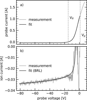
Figure 4. Comparison of the fitted theoretical I–V curve and the measurement at  and
and  . (a) Total probe current. (b) Ion current only. The curve marked 'measurement' is obtained by subtracting the calculated electron current from the measured total current.
Download figure:
Standard image High-resolution imageApart from the application of BRL to describe the ion current, the two other important theories, orbital motion limit (OML) and the theory of Allen, Boyd, Reynolds and Chen (ABR) were also evaluated [40–42]. However, only BRL was found to correctly describe the slope of the ion current. This might be due to the high ion energies found in HiPIMS [15, 43, 44], which would make the orbital motion of ions, which is included in BRL but not in ABR, very important [45].
Figure 5 shows the measured electron current, as derived from subtracting the calculated ion current from the measurement, together with the best fit, according to equation (1). Again, excellent agreement is found between fit and measurement. Summarizing, one can state that our analysis method produces very consistent results for the individual currents as well as for the complete probe current.

Figure 5. Electron current from the same measurement as figure 4. Calculated electron current according to equation (1) (fit) and the electron current that would be drawn by the probe for the given plasma parameters without a magnetic field (unmagnetized).
Download figure:
Standard image High-resolution imageThe good agreement between calculation and measurement validates the assumption of a Maxwellian EEPF. However, for the measurement closer to the target surface, at  , a change in the slope of the electron current can be observed for high energies. Consequently, the EEPF resembles more a bi-Maxwellian instead (not shown). Such a bi-Maxwelllian distribution has been predicted in literature to be caused by energetic secondary electrons [37]. However, this change in the slope always happens around the point where the ion current contribution to the total current becomes relevant. Furthermore, the electron current attributed to this hotter distribution is only around 1 mA. We thus conclude that this apparently bi-Maxwellian electron current is likely spurious and created by an imperfect fit of the ion current.
As a reference, figure 5 also shows the electron current which would be drawn to the probe at the given plasma parameters without a magnetic field present [34]:
The electron current for the magnetized case, however, is strongly reduced for small negative probe voltages or low electron energies, respectively. The diffusion parameter was found to be ψ0 = 12 in this measurement. Electron diffusion onto the probe is discussed in detail in the appendix. At high negative probe voltages, the magnetized and unmagnetized curves converge, as was recently also found by Ryan et al [18]. This observation can easily be explained by the fact that high energetic electrons have a large gyration radius and are, therefore, effectively not magnetized. In our experiments, such convergence happens at about 20 eV of electron energy, at which point the gyration radius of electrons rg is about the same as the diameter of the probe tip,  .
.
The plasma potential, as determined by the fit, is always between 1 V and 2 V more positive than the potential determined by the 'knee' method, using the position of the maximum of the first derivative of the electron current. This difference is caused by the magnetic field and is consistent with previous observations [46].
4. Results
4.1. Time evolution of plasma parameters
Figure 6 shows the temporal evolution of the plasma density at  during the discharge pulse as obtained by the time shift averaging method. On the right axis, the figure shows the total discharge current for comparison, averaged over 64 pulses. Breakdown occurs at about 18 μs, after which both current and plasma density begin to rise. The highest current is reached at the end of the discharge pulse, at
  , marked by the dotted, vertical line. The plasma density exhibits strong fluctuations corresponding to a rotating spoke structure moving past the probe. These fluctuations show the same pattern as in the PMT signal shown in figure 3, created by time shift averaging. The maximum density is obtained at the reference time of
  with a value of n = 6.6 × 10¹⁹ m−3. After that, the density drops sharply in about 600 ns to half that value, n = 3.2 × 10¹⁹ m−3. After the discharge pulse, both plasma density and current decay slowly and reach zero at about
  . This slow decrease of the current after the pulse is caused by the inductance in the power line that limits larger changes in current. Apart from the spoke fluctuations, the time evolution of plasma density and current agree surprisingly well. The amplitudes of the density fluctuations also agree very well with earlier estimates based on the measurement of fluctuations in the local target current density [21].
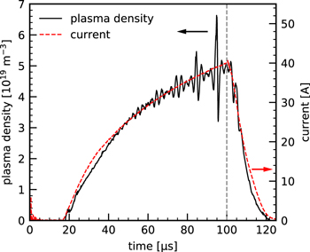
Figure 6. Plasma density development over the discharge pulse together with the total discharge current on the right axis. Measurement at  . The vertical line at 100 μs marks the end of the discharge pulse.
Download figure:
Standard image High-resolution imageFigure 7 shows the electron temperature (a) and the plasma potential (b) during the discharge pulse at  . The electron temperature first shows an oscillating behaviour after ignition, until it levels out at about 30 μs to a value of 3.3 eV. After that, the electron temperature decreases to about 2.6 eV at 60 μs. Later, spoke fluctuations become visible. Around the reference time of
  , the electron temperature rises inside the spoke up to 3.1 eV and then drops in about 1.5 μs to a value of 2.4 eV after the spoke.
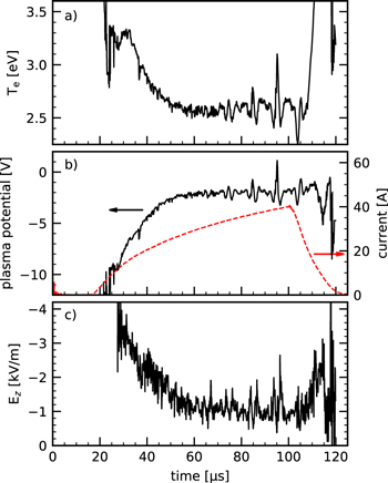
Figure 7. Electron temperature Te (a) and plasma potential (b) during the discharge pulse, for the measurement at  . (c) Electric field strength Ez, calculated from the difference between the plasma potentials at
  and
and  .
.
Download figure:
Standard image High-resolution imageFigure 7(b) shows the temporal evolution of the plasma potential with respect to ground during the discharge pulse. The plasma potential is strongly negative at about −10 V after ignition and then rises to about −2 V at about 60 μs. This value remains almost constant until the end of the discharge pulse apart from the spoke fluctuations. The plasma potential remains negative with respect to the ground potential at all times, except inside the spoke, where a positive plasma potential of 1 V is observed.
The overall spatial distribution of the plasma potential in the magnetic trap region has been measured previously [22, 47] and can be explained by the difference in electron and ion mobility. Since electron diffusion perpendicular to the magnetic field is greatly suppressed, the plasma potential is negative to confine the ions in order to maintain quasi-neutrality. As the discharge current and, therefore, the plasma density rises, electron mobility perpendicular to the magnetic field is enhanced by Coulomb collisions. Consequently, the plasma potential becomes more positive as more electrons are able to leave the magnetic trap region.
Figure 7(c) shows the electric field Ez, pointing towards the target surface, deduced from the difference in the measured potential at  and
and  (not shown). The electric field is initially very strong, with values of around −3500 V m−1 directly after ignition followed by a decrease to −1000 V m−1 at 60 μs. At later times, the electric field stays more or less constant until the end of the pulse apart from the spoke fluctuations. The temporal evolution of the electric field strength is, thus, essentially the same as for the electron temperature. It has been previously argued, that the electric field in the magnetic trap region is responsible for electron heating in HiPIMS [48]. The close agreement between the trends of the electric field strength and the electron temperature seems to confirm that Ohmic heating is indeed the most important electron heating mechanism at our conditions.
The evolution of the electric field strength, Ez, over the course of the pulse might also cause the slight discrepancy between the trends in current and plasma density, shown in figure 6. The initially higher electric field strength at the beginning of the pulse will pull ions more efficiently to the target implying a higher current at a given plasma density. This leads to a an initially slightly faster rise in current, compared to the plasma density, just after ignition.
4.2. Plasma parameters around ionization zones—the spokes
Figure 8 shows an enlarged view of the plasma parameters (n, Te, Vp) for all three spatial positions, around the reference time of  . Additionally, the figure shows the time shift averaged PMT time traces for all three positions as comparison at the bottom.

Figure 8. Zoom on the fluctuations in the plasma parameters caused by the main spoke at  for all three positions.
Download figure:
Standard image High-resolution imageThe electron density exhibits a slow increase at the leading edge of the spoke (at earlier times) and then drops sharply at the trailing edge. A higher density is found for measurements closer to the target surface, both inside and outside of the spoke. The maximum density is reached slightly before  with 9.7 × 10¹⁹ m−3, 8.2 × 10¹⁹ m−3 and 6.6 × 10¹⁹ m−3 for the measurements at
  , 8.0 mm, 9.7 mm, respectively.
In contrast, the electron temperature peak seems to be symmetrical, located slightly after  . Stronger fluctuations are visible for measurements closer to the target surface. The average electron temperature, however, changes only slightly. The strongest fluctuations are found for the measurement at
  . Here, Te is fluctuating between 2.1 eV and 3.4 eV.
The plasma potential peak is also located slightly after  . For measurements closer to the target surface, the plasma potential becomes more negative, as has been previously observed [22, 47, 49]. Inside the spoke, however, the plasma potential becomes more positive and the potential difference between the measurement positions become smaller. The electric field which is pulling ions to the target surface will thus be smaller inside the spoke, enabling ions to leave the magnetic trap region towards the substrate more easily. This can explain the increased ion current leaving the magnetic trap region, associated with spokes [10]. The potential peak is slightly asymmetrical, with a steeper slope at the trailing edge of the spoke. The azimuthal electric field can be calculated from the time derivative of the plasma potential Vp:

with the previously determined spoke velocity of  = 8.2 km s−1. For the measurement at
  , we find
  = 700 V m−1 at the leading edge of the spoke and
  = −1000 V m−1 at the trailing edge. It is interesting to note, that the electric field at the spoke edge, pointing in azimuthal direction, is thus about as strong as the electric field Ez outside the spoke, pointing towards the target.
The PMT time traces, shown at the bottom of the figure, agree well for all three positions. However, the measurement for the closest position shows slightly smaller fluctuations. This indicates that we might have indeed disturbed the plasma with the probe and might have slightly damped the spokes.
Our measurements can be compared to those of Lockwood Estrin et al, who find the same internal spoke structure: first a peak in plasma density at the leading edge of the spoke, and then a simultaneous peak in both electron temperature and plasma potential at the leading edge of the spoke [25]. Preliminary results, not presented here, indicate that this sequence of peaks is also found for titanium as the target material. Panjan and Anders did not obtain the plasma density for their measurement of spokes in DCMS. However, the authors also found the electron energy to peak simultaneously with plasma potential [24].
Our results also agree with spectroscopic imaging results obtained by A. Hecimovic at similar conditions [11]. There, the images show first a slow rise in intensity of the aluminium neutral lines around 396 nm at the leading edge of the spoke. At the trailing edge, a sharp peak in argon ion intensity was observed. This trend might very well correspond to the internal spoke structure observed here: the aluminium neutral lines, corresponding to low energetic ground state transitions, most likely follow the trend in electron density and thus peak first. The argon ion line transitions around 488 nm, however, correspond to excitation energies of around 20 eV follow rather the trend in the electron temperature. Hecimovic's spectroscopic results thus indicate the same internal spoke structure as our results.
The potential fluctuations (minimum to maximum) of about 7 V reported in this work are smaller than previous predictions by Anders et al for HiPIMS spokes (≈35 V [50]) or the measurements by Panjan and Anders for spokes in DCMS (≈70 V [24]). Additionally, we did not observe a strong positive plasma potential in the range of 15 V to 30 V relative to ground [13, 15], nor an electric field reversal in z direction, predicted by some authors [13, 15, 17, 51]. The post-processing in the time shift averaging method and the invasive nature of probe measurements might attenuate the measured potentials slightly, however it is unlikely for much stronger fluctuations or for positive potentials in the order of 20 V to remain undetected. The observed discrepancies might be explained by the choice of target material and discharge parameters. Additionally, both the present work and the work by Panjan and Anders [24] indicate that stronger potential fluctuations might be located even closer to the target surface.
The variation in plasma potential around the spokes is important for ion transport to the substrate. Figure 9 shows an illustration of the potential between target and substrate inside and outside of a spoke and is adapted from literature [13, 15, 17] but also updated in light of our measurements. The dots in the figure indicate the measured potential inside the spoke and in the minimum just before the reference spoke. The lines are an estimate regarding the spatial potential structure inside (solid line) and outside (dotted line) a spoke. The target sheath thickness is known to be around 100 μm and is thus not visible on the scale of figure 9 [21].
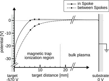
Figure 9. Illustration of the proposed potential structure between target and substrate inside and outside a spoke. Points indicate the measurements extracted from figure 8 at the potential minimum before the spoke (dotted line) and at the potential maximum at the trailing edge of the spoke (solid line). The target sheath is known to be about 100 μm thick under these conditions and thus not visible [21].
Download figure:
Standard image High-resolution imageThe potential structure as plotted in figure 9 demonstrates how the electric field pointing towards the target is largely reduced in the presence of a spoke. The potential barrier that ions have to overcome in order to leave the magnetic trap region is essentially mitigated by the presence of a spoke and ions may then diffuse unhindered towards the substrate. However, most of the ions will not be fast enough to leave the potential trap in the time span that the spoke is present. Most of the aluminium ions with mass  will have a velocity of around
  = 3500 m s−1, according to a Thompson distribution with
  [52]. That means that an ion can move approximately 1.8 mm during the time span of about 0.5 μs a specific spoke is present in front of a specific target location. After passing of the spoke, the ion will experience the electric field again, but it will have moved into a region further apart from the target where the electric field is already smaller. In this manner, the passing of several spokes during the transport time span of an ion traveling from the target surface to the substrate can induce an enhanced ion transport.
5. Conclusion
In this paper, we presented a method to average data collected over multiple HiPIMS pulses without losing spoke information. This method, called time shift averaging was applied to Langmuir probe measurements on an aluminium HiPIMS discharge. The probe current and the signal of a photo multiplier were simultaneously acquired by an oscilloscope and then spoke resolved I–V curves were recovered in post processing. The I–V curves were fitted with calculated curves including the effects of magnetized electrons in the calculations. In this way, the fluctuations in plasma parameters caused by the spokes were measured.
We found the plasma density to slowly rise at the leading edge of the spoke and then sharply drop at the trailing edge. For the measurement performed at the closest target distance of  we found a maximum density of n = 9.7 × 10¹⁹ m−3 and a subsequent drop to n = 3.8 × 10¹⁹ m−3.
The electron temperature, Te, was found to peak later at the trailing edge of the spoke. Fluctuations in Te became stronger, the closer the probe was moved to the target surface. For  , we measured Te to fluctuate between 2.1 eV and 3.4 eV.
The plasma potential was also found to peak at the trailing edge of the spoke. For  , the plasma potential was −6.9 V outside and 0.3 V inside the spoke. Outside the spoke, the plasma potential became less negative with target distance indicating a strong electric field of about
  = −1000 V m−1. However, inside the spoke no strong potential gradient was observed. In azimuthal direction, the electric field strength was
  = 700 V m−1 on the leading edge of the spoke and
  = −1000 V m−1 on the trailing edge.
The strong electric fields at the azimuthal edges of the spoke cause anomalous transport of electrons, which can then diffuse across the magnetic field lines and leave the magnetic trap region. Consequently, the plasma potential becomes more positive and the electric field towards the target is significantly reduced. Therefore, the potential barrier in the magnetic trap region that usually confines the ions is lifted and a sputtered ion may diffuse freely when the rotating spoke passes the sputtering location at the target surface.
This deconfinement effect may be the key to improve the efficiency of HiPIMS plasmas by reducing the return effect. Any direct control or triggering of spokes is then a method to control the deposition rate of HiPIMS.
Acknowledgments
The authors would like to thank Christian Maszl for the probe stem, Katharina Grosse for performing the magnetic field strength measurements, Ante Hecimovic for fruitful discussion and encouragement, Sascha Monje for experimental assistance and Michael Konkowski for help with designing the probe circuitry. Dennis Krüger and Denis Eremin are acknowledged for their advice on electron diffusion. This work has been funded by the DFG within the frame of the SFB-TR 87, project A5.
: Appendix. Electron diffusion across the magnetic field lines
The description of electron diffusion onto the probe against the direction of magnetic field lines follows the work of Arslanbekov et al and Popov et al [35, 36, 46].
For a probe placed parallel to the magnetic field lines, the diffusion parameter ψ, from equation (1), is:
with
and

Here, R, L and Ap are the radius, length and surface area of the probe, respectively. γ ≈ 1 is the geometric factor and W the total energy of the considered electron in the probe sheath. rg is the gyration radius of electrons and λ is the mean free path of electrons for momentum transfer collisions.
Direct application of equations (A.1) requires a highly accurate description of electron diffusion. Instead, we use the approximation  , which requires R ≫ b'. Since b' in turn depends again on the mean free path λ, an estimation of λ is necessary.
Coulomb collisions will be the most important type of collision, given the high plasma density present in our experiment. Since Coulomb collisions of identical particles give rise to little diffusion, we will only consider electron-ion collisions [53]. Assuming a background of heavy ions at rest, the cross section of such collisions are given by
for a single collision leading to a large scattering angle of 90° [54]. The cross section for many consecutive small angle collisions, leading to a large scattering angle is instead:
Usually, σm90 is the more important cross section. However, it is unclear if small angle collisions would really lead to much diffusion in the presence of a strong magnetic field. Using the mean free path  for both cross sections, the diffusion parameter ψ(B, W) can be calculated from equations (A.1).
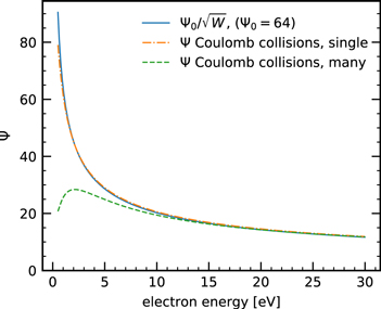
Figure A1 shows ψ as a function of electron energy W from equations (A.1) using the mean free path  with the cross sections from equations (A.2) (single) and (A.3) (many). Also shown is
  for ψ0 = 64. The calculations were performed for a plasma density of n = 5 × 10¹⁹ m−3, an electron temperature of
  and a magnetic field strength of
  . The approximation
  and the calculation with the cross section from equation (A.2) agree very well over the whole energy range. For the calculation with the cross section from equation (A.3), we find good agreement only for electrons with an energy
  . Consequently, the part of the electron current close to the plasma potential was de-emphasized in the fit. However, looking at figure 5, one can see that the electron current seems to be well described by the fit, using
  , even very close to the plasma potential. This might indicate, that many consecutive Coulomb collisions do indeed cause less diffusion in the presence of a strong magnetic field as one might expect.
Figure A1. Diffusion parameter ψ as a function of electron energy calculated using  (solid line) or using equation (A.1) together with the cross section from equation (A.2) (single) or equation (A.3) (many).
Download figure:
Standard image High-resolution image
It should be noted that the values of ψ0 obtained by the fit are much smaller than the value of ψ0 = 64 used in figure A1. Values found are rather in the range between 5 and 15. Presumable, this is indicative of anomalous transport. Assuming classical transport in the probe sheath and Bohm transport in the surrounding plasma, we can modify equations (A.1) by a factor of  [46]. The product of electron cyclotron frequency ωc and collision time τ, ωc τ is often used to quantify anomalous transport. For HiPIMS, values between 2 and 3 are expected [11, 55–57]. Here, values around ωcτ ≈ 2 create good agreement between the fitted ψ0 and the modified equations (A1).