

Abstract
A gliding arc (GA) plasma has great potential for CO2 conversion into value-added chemicals, because of its high energy efficiency. To improve the application, a 2D/3D fluid model is needed to investigate the CO2 conversion mechanisms in the actual discharge geometry. Therefore, the complex CO2 chemical kinetics description must be reduced due to the huge computational cost associated with 2D/3D models. This paper presents a chemistry reduction method for CO2 plasmas, based on the so-called directed relation graph method. Depending on the defined threshold values, some marginal species are identified. By means of a sensitivity analysis, we can further reduce the chemistry set by removing one by one the marginal species. Based on the so-called flux-sensitivity coupling, we obtain a reduced CO2 kinetics model, consisting of 36 or 15 species (depending on whether the 21 asymmetric mode vibrational states of CO2 are explicitly included or lumped into one group), which is applied to a GA discharge. The results are compared with those predicted with the full chemistry set, and very good agreement is reached. Moreover, the range of validity of the reduced CO2 chemistry set is checked, telling us that this reduced set is suitable for low power GA discharges. Finally, the time and spatial evolution of the CO2 plasma characteristics are presented, based on a 2D model with the reduced kinetics.
Export citation and abstract BibTeX RIS
1. Introduction
The increase of atmospheric CO2 concentrations has a growing detrimental effect on our climate and environment. Therefore, the conversion of CO2 into chemicals and fuels is one of the key fundamental challenges of the 21st century. A number of technologies have been developed to convert CO2 into value-added products [1, 2], such as photochemical, electrochemical and thermochemical pathways, either with or without catalysts, and all their possible combinations [3–9]. Another promising technology for CO2 conversion is the non-equilibrium plasma [10], which can induce chemical reactions at ambient temperature and pressure, because the electrons can activate the gas by electron impact excitation, dissociation and ionization. Moreover, as plasma can easily be switched on/off, it is very flexible and can adapt to the temporary storage of excess renewable energy during peak production. Most research on plasma-based CO2 conversion includes (packed bed) dielectric barrier discharges (DBDs) [11–19], microwave (MW) plasmas [20–26] and gliding arc (GA) discharges [27–35].
GA discharges are particularly interesting for CO2 conversion due to their high energy efficiency [36–39]. Indeed, the electrons typically have energy of about 1 eV, and this is most suitable for vibrational excitation of CO2 molecules, which is known to be the most energy efficient pathway for CO2 dissociation [40]. In the context of CO2 conversion, selective electron impact excitation to the vibrational levels can optimize the energy efficiency.
To investigate the mechanisms of CO2 conversion in GA discharges, 2D or even 3D fluid models are probably the most suitable approaches, as they can provide detailed information on the spatial behavior and on the effect of reactor geometry and gas flow dynamics. The combination of computational fluid dynamics and chemical kinetics can supply valuable information for experimental studies. However, such fluid models require a long calculation time, certainly in the case of complex CO2 chemistry kinetics, with detailed description of the vibrational levels, which are essential for understanding the CO2 conversion. Therefore, reduction of the CO2 detailed chemistry kinetics is quite important for the 2D/3D fluid models.
Chemistry reduction methods can be classified into three major categories: lumping, time scale analysis, and skeletal reduction [41, 42]. Lumping is most useful when there are some groups of reactants or products that have nearly the same chemical behavior, and each group can be treated as one pseudo-species. This method was already used to treat the asymmetric vibrational states of CO2 [43]. Time scale analysis uses various methods to define the highly reactive species or fast reactions in a reacting system, and approximate these as quasi-steady state species and partial equilibrium reactions. The corresponding differential equations are thus replaced with algebraic relations that can be solved explicitly to reduce the number of variables. The intrinsic low dimension manifold method [45] and computational singular perturbation method [46–48] are two systematic approaches of time scale analysis. Finally, skeletal reduction is the method to eliminate the species and reactions that are unimportant for the particular reaction conditions of the application.
The skeletal reduction method can be further categorized as reactions targeted or species targeted. The major methods for the elimination of reactions include sensitivity analysis [49, 50], principal component analysis (PCA) [51–53], and detailed reduction method [54, 55]. Sensitivity analysis is one of the earliest methods for skeletal reduction, PCA decouples different reaction groups, and species coupling was studied through Jacobian matrices such that species not strongly coupled to the major ones were eliminated [59]. However, these methods are typically time-consuming for large chemical mechanisms. The method of detailed reduction [54] can systematically identify the unimportant reactions by comparing its reaction rate with that of a pre-selected controlling reaction. The identification of the controlling reaction is however not easy, especially for large mechanisms, due to the lack of a universally rigorous definition of the controlling behavior.
Elimination of species can be achieved with methods such as Jacobian analysis [56, 57] and directed relation graph (DRG) [58]. The method of Jacobian analysis can identify species coupled with the important species. However, it requires an iterative procedure, and the selection of threshold values is arbitrary [57]. Therefore, the DRG method is applied to identify the unimportant species in this paper, since this method can generate skeletal mechanisms much faster than other available methods, and the resulting skeletal mechanisms can predict the reaction rates of the remaining species with a definable accuracy [58].
The DRG method proposed by Lu et al [58–60] made a significant breakthrough in chemistry reduction. It was designed to reduce large detailed mechanisms: species couplings are mapped to a graph and the species strongly coupled to the major species are identified. In other words, the DRG method comprises a set of directed paths that mark the species that will remain in the reduced mechanism. Since species are coupled through reactions, the definition of species relations in the DRG method starts from the rate expressions of the species and reactions in a detailed mechanism. Although this reduction method has been successfully applied in combustion simulations [61, 62], to our knowledge it has not been used in plasma modeling. The DRG method belongs to the flux analysis method, which is very fast, since the required time for calculating production and consumption rates is a small fraction of the time required to carry out the integration of the ordinary differential equation system. The reduced chemistry set based on flux analysis has errors bounded by the specified threshold value. When increasing the threshold value to obtain a very high level of reduction, the risk of losing critical species increases. Therefore, at the price of a higher computational demand, sensitivity-based reductions are able to further push the degree of reduction with an acceptable preservation of accuracy [63]. Hence, in our paper, we adopt the so-called flux-sensitivity analysis coupling method [63] for the reduction of the CO2 chemical kinetics.
This paper is organized as follows. In section 2, we first introduce the full CO2 plasma chemical kinetics model. Subsequently, in order to apply a 0D model to a GA plasma, we describe the plasma characteristics in a GA as input for the 0D model. Next we explain the DRG and sensitivity analysis methods. In section 3, we present the results of applying the DRG and sensitivity analysis methods to the CO2 plasma model. In order to properly use this reduced set, the range of validity of this reduced chemistry set is given in section 4. The reduced set of the CO2 kinetics model applicable to a 2D/3D GA model is presented in section 5, and the time and spatial evolution of the plasma characteristics are presented. Finally, the conclusions are given in section 6.
2. Description of the model
2.1. 0D chemical kinetics model
The model used in this work is a 0D model, which solves the time-evolution of the species densities by balance equations, taking into account the various production and loss terms by chemical reactions. We use an existing code ZDPlaskin [64], which features an interface for description of the plasma species and reactions, a solver for the set of differential equations and a Boltzmann equation solver BOLSIG+ [65]. In this 0D model, transport processes are not explicitly considered, since a 0D model only calculates the species densities as a function of time. Nevertheless, the transport of the arc through the GA reactor can be mimicked by translating the temporal behavior, as calculated in the model, into a spatial behavior, corresponding to the position in the reactor, by means of the gas flow rate. This allows us to mimic the typical plasma evolution behavior of a GA used for CO2 conversion [66].
The comparison of the calculated conversion and energy efficiency with experimental values for the same conditions in our previous work [66] indicates that the detailed chemistry set used in this model is generally reasonable for a GA discharge, although there is no guarantee that the kinetics of all species are correct, as the latter can only be concluded from direct validation of the chemistry of those particular species with experiments. Seventy-two different species are considered in the model. Figure 1 shows the energy diagram of the CO2 vibrational levels included in the model. The energies of the CO2 vibrational levels can be calculated using the anharmonic oscillator approximation. We consider the four lowest effective symmetric mode levels (denoted by letters) and 21 asymmetric mode levels (denoted by numbers) up to the dissociation limit of the molecule. The chemical reactions include electron impact reactions, vibrational energy transfer reactions and heavy particle reactions leading to breaking and formation of new species. For more detailed information about the reactions and the rate coefficients used, see [67–70].
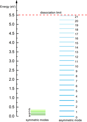
Figure 1. Effective energy levels of CO2 included in the model, i.e. four symmetric mode levels (denoted by letters a–d), 21 asymmetric mode levels (denoted by numbers 1–21) and the CO2 ground state (denoted by 0).
Download figure:
Standard image High-resolution image2.2. Plasma characteristics in a GA, as input for the 0D model
In a GA discharge, the arc is ignited at the shortest interelectrode gap when the electric field is high enough to cause breakdown. Then the arc expands upwards along the surface of the electrodes upon effect of the gas flow, and elongates until it extinguishes [71]. Although a 0D model cannot describe the increase of arc length from the shortest gap to a larger gap, we can use the time evolution of the plasma parameters as input, which are related to the increase of arc length during the arc downstream movement. Indeed, the gas molecules move together with the arc on their way throughout the reactor. This is thus taken into account in the model by translating the spatial variations of the plasma characteristics in the reactor into temporal variations, to be used as input in the model, as described below.
The power density is assumed to be constant with time in the region between the electrodes where the arc is formed. This assumption is justified from our previous calculations [66]. The electric power in the plasma is applied to the electrons by setting a certain value for the reduced electric field (E/N, i.e. ratio of electric field over gas density). The reduced electric field is calculated at each time step, to keep the desired power density due to the changing gas composition as a function of time (upon CO2 conversion into CO and O2). We consider a power density of 10 kW cm−3. In our model the power density in the arc zone (i.e. the region between the electrodes) is calculated as the plasma power divided by the arc volume. It is reported in literature that the GA is a plasma string with a diameter of about 1 mm, surrounded by a weakly ionized zone [72, 73]. Thus, in our 0D model the arc volume is seen as a cylinder with a diameter of about 1 mm. Therefore, at an applied power on the order of tens of watts [66], the arc column diameter is usually about 1 mm [72, 73], and the arc length is on the order of the interelectrode distance, hence around 1–3 mm [66]. This results in an arc column volume in the order of 10−3 cm3, and thus the power density is in the order of 104 W cm−3. In practice, the plasma parameters are not uniformly distributed due to the plasma arc core surrounded by a weakly ionized zone. So the power density should be high in the arc core, and low in the arc fringe region. Hence, the magnitude of the power density in our model, which applies to the arc zone, may be achieved in practice. Moreover, it yields an electron density and electron temperature (see figure 2), in agreement with experimental values in the order of 1018 m−3 and 1–2 eV, respectively [74, 75]. In the region beyond the electrodes, i.e. during the post-discharge stage, the power density is set to zero, and thus, both the electron density and electron temperature also drop to zero, as is clear from figure 2. In this study, we set the arc time as 8 ms based on the GA cycle in the experiments, and the total gas residence time is assumed to be 15 ms, which is sufficient for relaxation of the reactive species to equilibrium. In the calculation, the gas pressure is kept constant at one atmosphere.
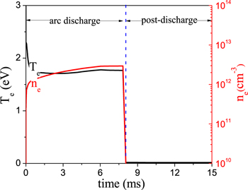
Figure 2. Calculated electron temperature and electron density as a function of time at a power density of 10 kW cm−3.
Download figure:
Standard image High-resolution imageThe time-resolved temperature distribution in figure 5 is based on the combination of experimental measurements and modeling, since the experimental measurements did not provide a time-resolved gas temperature distribution. The maximum temperature 2600 K in figure 5 is obtained according to a measured time-space averaged temperature in the experiment [78]. The gas temperature profile in figure 5 is assumed based on our earlier findings [76]. The gas temperature first increases with time during the arc downstream movement, and then almost stays constant in our previous 3D model results [76], as presented in figure 3. The geometry used in the 3D modeling is presented in figure 4, which shows a cross section through the middle of the anode and the cathode [76]. A pair of semi-ellipsoidal electrodes are 50 mm long and the shortest interelectrode distance is 3.2 mm in the model. The entire geometry, including the region outside the electrodes where the gas can flow without passing through the arc, is a cylinder, with radius of 31.8 mm and length of 150 mm. Note that the gas temperature plotted in figure 3 was obtained for argon, and it is higher in a CO2 discharge, due to the vibration-translation (VT) relaxation processes [44]. Therefore, in our 0D model for CO2 we consider a fixed gas temperature profile, increasing from 300 to 1000 K in the first 0.05 ms, due to the short characteristic time (10−5 s) for VT relaxation processes [67]. Subsequently, until 6 ms, the gas temperature increases further to a maximum value of 2600 K, which is based on experimental measurements from literatures [77, 78], and then it stays constant during the rest of the arc stage (see figure 5). From our previous 3D results, in the post-discharge region, the electron density and electron temperature suddenly drop to negligible values, while the gas temperature gradually decays [76]. Therefore, after the gas leaves the arc, the gas temperature profile is assumed to gradually decrease to 500 K, which corresponds to the outlet gas temperature measured in the experiments [66].
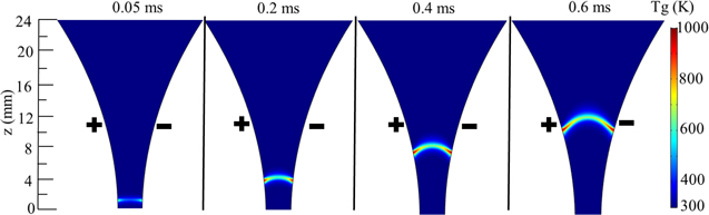
Figure 3. Time and spatial evolution of the gas temperature in the interelectrode gap for a GA in argon, at a current of 28 mA and a gas flow rate of 10 l min−1, as obtained from our earlier 3D fluid modeling results [76]. The electrodes are indicated with + (positive) and − (negative) symbols.
Download figure:
Standard image High-resolution image
Figure 4. The Cartesian geometry used in 3D model [76].
Download figure:
Standard image High-resolution image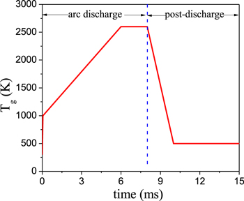
Figure 5. Gas temperature profile as a function of time, at a power density of 10 kW cm−3.
Download figure:
Standard image High-resolution image2.3. DRG method
The theory of DRG is well suited to abstract the coupling among the species. Specifically, each node in a DRG represents a species in the full chemistry, and there exists an edge from vertex A to vertex B, if and only if the removal of species B would directly induce a significant error to the production rate of species A. That is, an edge from A to B means that B has to be kept to correctly evaluate the production rate of A [58–60].
The expression of the production rate of species A is:


where summation is made over all production reactions,  is the stoichiometric coefficient of species A in the reaction i,
  is the production rate, expressed by equation (2), where ki is the reaction rate constant, and
  is the density of the lth reactant in reaction i.
To quantify the direct influence of one species on another, a normalized contribution of species B to the production rate of species A can be defined as [58]:

 if the ith elementary reaction involves species B,
  otherwise.
If the normalized contribution rAB is sufficiently large, the removal of species B from the chemistry set is expected to induce significant error on the production rate of species A. Consequently, if A has to be kept, B should also be kept. In such a case, we conclude that species A strongly depends on species B.
To quantify the dependence of A on B, we define a small threshold value ε such that, for rAB < ε, the dependence can be considered negligible. In this paper, a relatively large value ( ) and a small value (
 ) are used to quantify the dependence of one species on another, for the reason explained in next section. Note that
  is a typical value that can be used in most cases [42]. In other words, species A depends on species B if and only if there exists a directed path from A to B in DRG, i.e. B is reachable from A. For each species A, there exists a group of species, which are reachable from A, and this set of species is defined as the dependent set of A, denoted as SA. If species A is an important species to be kept in the reduced mechanism, its dependent set SA should be kept as well.
This method is practically used as follows: first the reactions in which the target species participated are selected, and then the production rate of target species can be calculated. For each species involved in these reactions, the relative contribution of each species to the target species is calculated. Finally the relative contributions larger than the specified threshold value ε are exported, and the graphs (figures 6, 7, 9 and 10) are plotted manually. For even larger sets of species and reactions, a graph searching method, such as so-called 'depth first search', which features a linear searching time proportional to the number of edges in the graph, can be exploited to find all the vertices reachable from the starting species.

Figure 6. Directed relation graph for CO2 as target species, based on a threshold value ε = 0.2. The numbers next to the arrows indicate the normalized contributions of one species to the formation and loss reactions of the other species (see text).
Download figure:
Standard image High-resolution image2.4. Sensitivity analysis to CO2 conversion
It is pointed out in [79] that a detailed reaction model is composed of three types of species: critical, nonessential, and marginal species. Critical species participate in those reaction channels that largely determine the simulation results, while nonessential species participate in reaction channels having little to no influence on the simulation results. A successful reduction model retains all critical species, eliminates all nonessential species, and properly deals with the marginal ones.
Based on the DRG method, different species are chosen when adopting different threshold values, and therefore, there exist some nonessential species, which are not involved in these important reaction channels, and also some marginal species depending on the desired accuracy, in our case the size of the threshold value. These nonessential species can be straightforwardly removed from the full reaction set. However, when using the above DRG method to obtain a significant reduction by increasing the threshold value ε, the risk of losing critical marginal species increases. So for these marginal species, a further reduction can be achieved using the more time-consuming sensitivity analysis method to evaluate their effects on the target property. By means of a sensitivity analysis, we can calculate the error on a defined target property, following the removal of each of the marginal species, and ranking them accordingly [63]. In our work, we use several quantities as the investigated target property, i.e. the calculated CO2 conversion, the electron density and the densities of the major neutral species, as well as the vibrational distribution function (VDF) of CO2. Starting from the reduced chemistry set obtained through the DRG method, the species to be investigated are detected by fixing different threshold values. Once marginal species are detected, they are ranked according to the error induced by their removal: for the ith species, the error is evaluated as

where XDET,i and XRED,i are the target property before and after the removal of species i, respectively. In this way, the species are ranked according to the induced error and can then be progressively removed from the chemistry set obtained in section 2.3.
3. Results and discussion
3.1. Reduced chemistry set
3.1.1. Role of species in CO2 production and loss
In the following DRGs (figures 6, 7, 9, 10), the blue circles represent the neutral species, and the green squares represent charged particles. The species marked red in blue circles and green squares are the marginal species. The direction of the arrows means a direct dependence of one species on another, measured by equation (3), for example, CO2 → CO, as shown in figure 6, can be considered as the dependence of species CO2 on CO, including both source and loss terms. When different species depend on the same species, this species will appear multiple times in the same figure.
We start from CO2 as the major species, and the other species reachable from CO2 can be searched. Figure 6 shows the resulting species relation graph, in which each directed edge represents a direct dependence of one species on another. The numbers on the directed edges represent the time-integrated normalized contributions of one species to the production and loss rate of the major species, calculated by equation (3). If this number would be 1, it would mean that this species is involved in every loss and formation reaction of the other (major) species. Usually, this is not the case, so the number on the directed edge is typically lower than 1.
The species relations smaller than a critical value ε = 0.2 are neglected in figure 6. It can be clearly seen that CO2 strongly depends on CO and O, while CO and O are also strongly coupled, and both depend on the electrons and the CO2 vibrational states. Here we should note that CO2(V) includes both four effective symmetric mode levels and the 21 asymmetric mode vibrational states up to the dissociation limit (see details in [67, 68]). Therefore, we can conclude that CO2, CO, O, CO2(V) and the electrons are the important species, which should be included in the reduced chemistry set.
In order to avoid losing critical species, we can reduce the threshold value ε to include more species. Figure 7 shows the DRG based on a threshold value ε = 0.02. Compared with figure 6, the species marked in red and the arrows marked in orange are newly added in this figure, i.e. O2, the vibrational states of CO and O2, the electronically excited state CO2(e), and negative ions CO3−, O2−, which are considered as marginal species. In order to analyse the effect of the removal of these species on the CO2 conversion, a sensitivity analysis is performed in the next section.

Figure 7. Directed relation graph for CO2 as target species, based on a threshold value ε = 0.02. The numbers next to the arrows indicate the normalized contributions of one species to the formation and loss reactions of the other species (see text).
Download figure:
Standard image High-resolution imageFigure 8 presents the relative contributions of the most important reactions responsible for the CO2 loss and formation. The main loss reaction is electron impact dissociation of vibrationally excited states of CO2 into CO and O, while the reaction of CO (either in the ground state or in vibrationally excited states) with O atoms and a third body (M) is the predominant production process of CO2. Moreover, electron impact dissociation of ground state CO2 and dissociation of vibrationally excited states of CO2 upon collision with O atoms are also quite important CO2 loss processes, with a relative contribution of 15% and 13%, respectively, while the recombination of CO with O2 also contributes to CO2 formation, with a relative contribution of 9%.
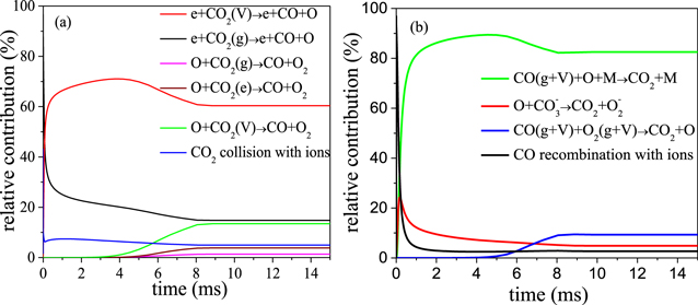
Figure 8. Relative contributions of the most important reactions responsible for the CO2 loss (a) and formation (b).
Download figure:
Standard image High-resolution image3.1.2. Role of species in sustaining the arc
From our previous paper [66], we know that charged particles almost have no contribution to the loss and production of CO2, and this finding is also consistent with our results in figure 8. However, the charged particles are very important to sustain the arc, as revealed by our 2D/3D model, especially the electrons. Thus, we now take the electrons as the target species, to reveal which species are reachable from the electrons. The result is presented in figure 9 for the species with normalized contribution above a threshold value ε = 0.2. The directed edges indicate that the electrons strongly depend on the negative ions O2−, O−, and neutral species CO2, CO, O2, O, C. The numbers next to the arrows indicate the contribution of each species to the electron production and consumption rates calculated by equation (3). The red arrow to CO2+ indicates that its contribution is larger than 0.2 at the beginning, although the normalized contribution integrated over the entire gas residence time is below 0.2.
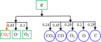
Figure 9. Directed relation graph for the electrons as target species, based on a threshold value ε = 0.2. The numbers next to the arrows indicate the normalized contributions of one species to the formation and loss reactions of the other species.
Download figure:
Standard image High-resolution imageSince there are many ions in the full chemistry set [67, 69], we reduce the threshold value ε in order to avoid losing the critical ions. Figure 10 shows the DRG for the target species reachable from the electrons, based on a threshold value ε = 0.01. The positive ions and neutral species marked in red are newly added, and are considered as marginal species. It can be seen that CO4+ ions have a contribution to the production and loss of electrons at a small threshold value, as shown in figure 10. The CO4+ ions are formed by the O2+ ions conversion reaction (O2+ + CO2 + M → CO4+ + M), so the relative contribution of O2+ ions to the production of CO4+ ions is calculated. It is found the O2+ ions are strongly coupled to the CO4+ ions although they have a negligible direct contribution to the electrons. So these two ions should be retained together in the reduced chemistry set. The other ions not included here (such as CO+, CO4−, O4+, O4−, O3−, O+, C2O2+, C2O3+, C2O4+, C2+, C+), and their chemical reactions, can safely be removed from the full chemistry set. In the next section we will employ sensitivity analysis to evaluate the effect of removing these marginal species one by one on the CO2 conversion. In this way, we can assure whether these marginal species should be kept in the final reduced chemistry set or not.
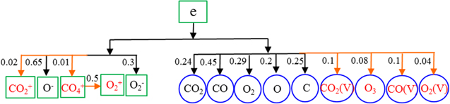
Figure 10. Directed relation graph for the electrons as target species, based on a threshold value ε = 0.01. The numbers next to the arrows indicate the normalized contributions of one species to the formation and loss reactions of the other species.
Download figure:
Standard image High-resolution image3.2. Sensitivity analysis: effect of the chemistry reduction on the CO2 conversion
Combining the above analysis in sections 3.1.1 and 3.1.2, we obtain a reduced chemistry set, including the following neutral and charged species: CO2, CO2(V), CO2(e), CO, CO(V), O2, O2(V), O3, O, C, CO2+, CO4+, CO3−, O2+, O2−, O−, and the electrons. Since different threshold values result in different species in the reduced set, we apply sensitivity analysis to evaluate the effect of removing these marginal species (marked in red in figures 7 and 10) one by one on the CO2 conversion. Figure 11 shows the results for removing the marginal species one by one, for seven different cases (see legend). We observe in this figure a double knee in the post-discharge stage. In the time range from 8 to about 9 ms, the CO2 conversion drops faster, while the drop becomes slow between 9 and 10 ms. This phenomenon is a physical effect related to the variations of gas temperature. As shown in figure 5, the gas temperature is below 1500 K at about 9 ms, so the three-body recombination rate of CO with O atoms and a third body M decreases, resulting in a slow drop in conversion value after about 9 ms. From this figure we can deduce that the CO2 conversion predicted by the magenta and green lines greatly deviates from the conversion obtained by the full reaction set, which means that O2+ and CO2(e) should be kept in the reduced chemistry set. In order to check whether these species are responsible for the large changes seen when they are removed additionally to other species, figure 12 below shows the effect of removing only O2+ species on the CO2 conversion. The result is the same as in figure 11 (i.e. no CO3−, CO4+ and O2+). Therefore, it can be inferred that the O2+ species is the one responsible for the large changes seen when it is removed additionally to other species. It is clear that for the other cases the CO2 conversion obtained with the reduced chemistry sets agrees well with the full reaction set, for the entire gas residence time. The maximum error is about 7% in the arc stage and 1% in the relaxation stage. Thus, the obtained reduced chemistry set, including only CO2, CO2(V), CO2(e), CO, O2, O, C, CO2+, O2+, O2−, O−, and the electrons, is suitable to predict the CO2 conversion in our GA, at the discharge condition investigated.
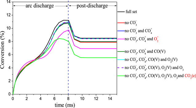
Figure 11. Effect of removing the marginal species one by one on the CO2 conversion.
Download figure:
Standard image High-resolution image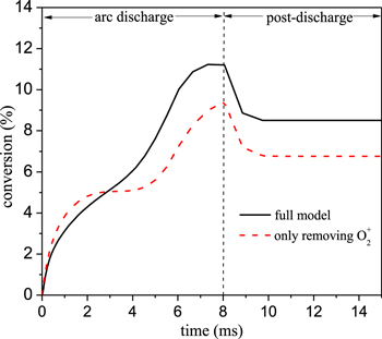
Figure 12. Effect of removing only the O2+ species on the CO2 conversion.
Download figure:
Standard image High-resolution image3.3. Sensitivity analysis: effect of the chemistry reduction on other plasma properties
The CO2 conversion as the sole target property is not a guarantee for the reliability of this chemistry set and for the effect of the chemistry reduction on all other plasma properties. Indeed, the effect on other important properties, like the densities of the various plasma species, should also be evaluated.
Comparison of the densities of the various neutral species predicted by both the full chemistry set and the reduced set is shown in figure 13. The densities of the neutral species obtained with the reduced chemistry set are in good agreement with those obtained with the full chemistry set in the arc stage. In the post-discharge stage, the densities of CO2, CO and O2 molecules are the same for the reduced and full chemistry sets, while the density of O is different from that obtained with the full set, but its density is low, and it has no influence on the CO2 conversion. In general, the densities of the neutral species obtained with the reduced set are basically in good agreement with those obtained with the full chemistry set.
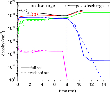
Figure 13. Comparison of the reduced and full chemistry set for the densities of the neutral species.
Download figure:
Standard image High-resolution imageFor the density of charged species, the positive ions density predicted by the full set is higher than that obtained by the reduced set at the beginning, and the positive ions density becomes close to that obtained by the reduced set with the increase of time. The ions have very little direct effect on the CO2 conversion and are therefore only important for determination of the electron density. So the comparison of electrons density between the reduced and full chemistry set is shown in this study.
Figure 14 presents the comparison of the CO2 asymmetric VDF predicted by the full set and the reduced set both in the arc discharge and in the post-discharge. The time for the arc discharge is at the end of the discharge, i.e. t = 7.6 ms, and the time for the post-discharge is at t = 8.5 ms. The reduced set predicts a slightly underestimated density for the first eight vibrational levels, but in general the agreement is very good, both in the arc stage and in the post-discharge stage. As the reduced chemistry set does not account for the CO vibrational levels, while the full chemistry set considers 10 CO vibrational levels [67], this shows that, under this condition, the CO vibrational levels do not affect the CO2 VDF.
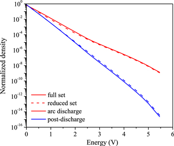
Figure 14. Comparison of the reduced and full chemistry set for the CO2 vibrational distribution function.
Download figure:
Standard image High-resolution imageFigure 14 suggests that we can use an additional reduction method to further reduce our chemistry set. Indeed, in [43], a level lumping method was proposed to treat the asymmetric mode vibrational levels of CO2 in order to reduce the calculation time. In [43] the VDF was not in thermal equilibrium and showed a plateau for the intermediate vibrational levels; it could be represented by three groups in the lumped level method, but figure 14 illustrates that for the conditions investigated here, the CO2 vibrational levels follow almost a Boltzmann distribution, so that one group is sufficient to describe the 21 CO2 asymmetric mode vibrational levels. This is indeed what we will do in the 2D model explained in section 5 below. Note also that the VDF, and thus the vibrational temperature (being a measure for the population of the first vibrational level of CO2) is higher in the arc discharge than in the post-discharge, indicating that the vibrational levels are more populated in the arc discharge than in the post-discharge, which is indeed like expected.
Figure 15 compares the electron density predicted by the full set and the reduced set. The electron density predicted by the reduced set is slightly lower in the arc stage, but in the post-discharge stage, the electron density quickly drops to zero for both chemistry sets. The maximum error in the electron density is about 12% in the arc stage. Because many positive and negative ions are included in the full set, it is difficult to obtain exactly the same electron density with the reduced and full sets. On the other hand, this difference almost has no influence on the CO2 conversion, so the agreement between the full set and reduced set is very good.
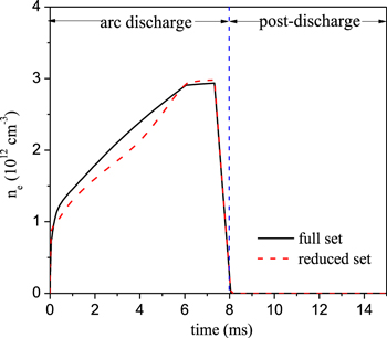
Figure 15. Comparison of the reduced and full chemistry set for the electron density.
Download figure:
Standard image High-resolution imageFinally, we compare in figure 16 the reduced electric field obtained by both the full chemistry set and the reduced set. The reduced electric field predicted by the full set remains almost constant at about 67 Td in the arc stage, while the value obtained by the reduced set is slightly higher, and decreases to about 67 Td at the end of the arc stage. In the post-discharge stage, the reduced electric field quickly drops to zero for both chemistry sets. In general, the reduced electric field obtained with the reduced set is in good agreement with that obtained with the full chemistry set.

Figure 16. Comparison of the reduced electric field, as obtained by the reduced and full chemistry set.
Download figure:
Standard image High-resolution image4. Range of validity of the reduced model: effect of power density
From the results above, it is clear that the reduced chemistry set is able to reproduce the results obtained with the full chemistry set, at the discharge condition studied in this paper.
Counting for the number of equations to solve, only taking into account the chemical kinetics part of the model, the full chemistry set from [67, 69] requires to solve 72 equations, while the reduced chemistry set only has to solve 36 equations (when including all 21 asymmetric mode vibrational levels of CO2; and 16 equations when these levels are lumped into one group). This greatly reduces the computational cost.
Despite the clear advantages of the reduced set, it should be stressed that it might not be valid under all conditions that can exist in a GA CO2 plasma. Therefore, we also need to test the validity of the reduced chemistry set for more extreme conditions, to assess its range of applications. For low power GA discharge, the power densities of 6, 15, 20 and 30 kW cm−3 are used in this study. In this power density range, the plasma power changes from about 14 to 70 W when the shortest interelectrode distance is about 3 mm, since the plasma power is calculated as the power density multiplied by the arc volume, which can be seen as a cylinder with a diameter of about 1 mm.
In figure 17 we compare the CO2 conversion predicted by the full set and the reduced set at different power densities (6 kW cm−3, 15 kW cm−3, 20 kW cm−3 and 30 kW cm−3, respectively). At the low power densities of 6 and 15 kW cm−3, the conversion predicted with the reduced set is in good agreement with the full set. With increasing power density, the difference of CO2 conversion between the full set and the reduced set increases. As shown in figure 17(b), the maximum error in the arc stage at 20 kW cm−3 increases to 18% at the time of about 5 ms, while at 30 kW cm−3, a somewhat larger difference is observed, with a maximum error in the arc stage of about 30%. Therefore, the reduced set seems not applicable at power densities larger than 30 kW cm−3. The reason is that at a larger power density, the conversion in the arc increases, resulting in relative high number densities of CO and O2, so the contribution of their vibrational levels may not be negligible anymore. In this case, a reduced set with more vibrational species should be used.
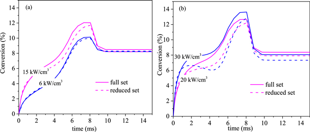
Figure 17. Comparison of the conversion predicted by the full set (solid lines) and the reduced set (dashed lines) at four different power densities.
Download figure:
Standard image High-resolution imageFurthermore, the difference in the conversion can also be explained from the difference in the electron density predicted by the two chemistry sets, as presented in figure 18. At 30 kW cm−3, the electron density is somewhat lower in the reduced model (maximum error of 25%), resulting in a lower CO2 conversion. When more ions would be added to the reduced model, like CO+ and O+, the agreement would be better, since a larger power density results in more ionization. In order to see the effects of ions on the conversion, the CO2 conversion with more ions in the reduced chemistry set is presented in figure 19 below. The extra ions added to the reduced chemistry set include CO+, O+, and C2O2+. It can be seen from figure 19 below that the CO2 conversion increases with more ions included, due to the increase of the electron density.
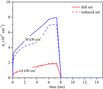
Figure 18. Comparison of the electron density predicted by the full set (solid lines) and the reduced set (dashed lines) at a power density of 6 and 30 kW cm−3.
Download figure:
Standard image High-resolution image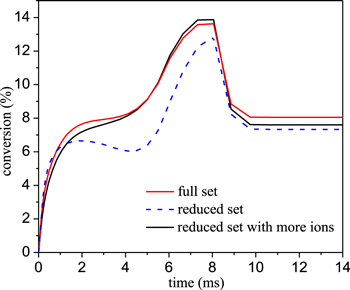
Figure 19. Comparison of the conversion predicted by the full set and different reduced sets at a power density of 30 kW cm−3.
Download figure:
Standard image High-resolution imageBased on the above analysis, the range of applicability of the reduced model is discussed. In the model the gas processing time in the arc is assumed to be 8 ms based on the arc cycle, and we set the total time in our calculations as 15 ms, which is sufficient, because the gas composition does not change with time anymore, so it has no influence on the conversion. Usually a pair of semi-ellipsoidal electrodes is used in conventional GA discharges, with the shortest interelectrode distance around 1–3 mm. Since in our 0D model the arc volume is seen as a cylinder with a diameter of about 1 mm, the arc column volume is about 2.35 × 10⁻³ cm3 when the arc is close to the shortest interelectrode position with the shortest interelectrode distance around 3 mm. So at the power density of 30 kW cm−3, the discharge power is about 70 W. Therefore, it indicates that the reduced chemistry set is applicable for low power CO2 GA discharge with the arc cycle in the order of milliseconds.
5. Reduced chemistry set for a 2D CO2 model in a GA
5.1. Reduced CO2 chemistry reactions
In previous section we have validated the reduced chemistry set for CO2 conversion in a GA by comparing various calculation results with the full chemistry set. Table 1 lists the species included in the reduced chemistry set, and tables 2–5 present the corresponding chemical reactions. In this section, this reduced chemistry set is applied to a 2D model for a GA.
Table 1. Species described in the reduced chemistry model.
| Molecules | Charged species | Radicals | Excited species |
|---|---|---|---|
| CO2, CO, O2, | CO2+, O2+, O−, e, O2− | O, C | CO2(Va, Vb, Vc, Vd), CO2(e) |
| CO2(V1)...CO2(V21) |
Table 2. Electron impact reactions included in the reduced chemistry model, calculated with cross section data, using the calculated EEDF.
| No | Reaction |
|---|---|
| (X1) | e + CO2 → e + e + CO2+ |
| (X2) | e + CO2 → e + CO + O |
| (X3) | e + CO2 → CO + O− |
| (X4) | e + CO2 → e + CO2Vx |
| x = a, b, c, d | |
| (X5) | e + CO2Vi → e + CO2Vj |
| (X6) | e + CO2 → e + CO2(e) |
| (X7) | e + CO → C + O− |
| (X8) | e + CO → e + C + O |
| (X9) | e + O2 → e + O + O |
| (X10) | e + O2 → e + e + O2+ |
| (X11) | e + O2 → O + O− |
Table 3. Ion reactions included in the reduced chemistry model, as well as the corresponding rate coefficients, in m3 s−1 and m6 s−1, for two-body and three-body reactions, respectively. Tg and Te are given in K and eV, respectively.
| No | Reaction | Rate coefficient |
|---|---|---|
| (E1) | e+CO2+ → CO + O | 4.2 × 10⁻¹³(1.16 × 10⁴Te/300)−0.75 |
| (E2) | e+CO2+ → C + O2 | 3.94 × 10⁻¹³Te−0.4 |
| (E3) | e+O + M → O− + M | 1 × 10−43 |
| (E4) | e+O2+ + M → O2 + M | 1 × 10−38 |
| (E5) | e+O2+ → O + O | 6 × 10⁻¹³(1/Te)0.5(1/Tg) 0.5 |
| (E6) | O2− + M → O2 + M + e | 2.7 × 10⁻¹⁶(Tg/300)0.5exp(−5590/Tg) |
| (E7) | O + O2− → O2 + O− | 3.31 × 10⁻¹⁶ |
| (E8) | O− + M → O + M + e | 4.0 × 10⁻¹⁸ |
| (E9) | O− + O → O2 + e | 2.3 × 10⁻¹⁶ |
| (E10) | O− + O2+ → O2 + O | 2.6 × 10⁻¹⁴(300/Tg)0.44 |
| (E11) | O− + O2+ → O + O + O | 4.2 × 10⁻¹³(300/Tg)0.44 |
| (E12) | O2+ + O2− → O2 + O2 | 2.01 × 10⁻¹³(300/Tg)0.5 |
| (E13) | O2+ + O2− → O2 + 2 O | 4.2 × 10⁻¹³ |
| (E14) | CO + O− → CO2 + e | 5.5 × 10⁻¹⁶ |
| (E15) | e+O2 + M → O2− + M | 3.0 × 10−42 |
Table 4. Neutral–neutral reactions included in the reduced chemistry model, as well as the corresponding rate coefficients, in m3 s−1 and m6 s−1, for two-body and three-body reactions, respectively. Tg is given in K.
| No | Reaction | Rate coefficient |
|---|---|---|
| (N1) | M + CO2 → M + O + CO | 1.81 × 10⁻¹⁶exp(−49 000/Tg) |
| (N2) | O + CO2 → CO + O2 | 2.8 × 10⁻¹⁷exp(−26 500/Tg) |
| (N3) | CO2 + C → CO + CO | 1.0 × 10⁻²¹ |
| (N4) | C + O2 → O + CO | 3.0 × 10⁻¹⁷ |
| (N5) | O + C + M → M + CO | 2.14 × 10−41(Tg/300)−3.08exp(−2114/Tg) |
| (N6) | CO + O2 → CO2 + O | 4.2 × 10⁻¹⁸exp(−24 000/Tg) |
| (N7) | CO + O + M → CO2 + M | 8.2 × 10−46exp(−1510/Tg) |
| (N8) | O + O + M → O2 + M | 5.2 × 10−47exp(900/Tg) |
Table 5. Neutral reactions between vibrationally excited molecules included in the reduced chemistry model, as well as the corresponding rate coefficients, given in m3 s−1 and m6 s−1, for two-body and three-body reactions, respectively. Tg is given in K.
| No | Reaction | Rate coefficient |
|---|---|---|
| (V1) | CO2 Va +M → CO2 + M | 7.14 × 10⁻¹⁴exp(−177Tg−1/3 + 451Tg−2/3) |
| (V2) | CO2V1 + M → CO2 Va +M | 4.25 × 10⁻⁷exp(−407Tg−1/3 + 824Tg−2/3) |
| (V3) | CO2V1 + M → CO2 Vb+M | 8.57 × 10⁻⁷exp(−404Tg−1/3 + 1096Tg−2/3) |
| (V4) | CO2V1 + M → CO2 Vc+M | 1.43 × 10⁻¹¹exp(−252Tg−1/3 + 685Tg−2/3) |
| (V5) | CO2V1 + CO2 → CO2Va+CO2Vb | 1.06 × 10⁻¹¹exp(−242Tg−1/3 + 633Tg−2/3) |
| (V6) | CO2V1 + CO2 → CO2 + CO2V1 | 1.32 × 10⁻¹⁶(Tg/300)0.5250/Tg |
A reduced non-equilibrium CO2 plasma chemistry set is also proposed in [43]. The difference is that CO3− and O2(V) are included in [43] and O2+ is included in our reduced chemistry set. This can be explained by the fact that at our conditions, the electron temperature is higher, resulting in more ionization, so the O2+ ions cannot be neglected, which also can be seen from its effect on the CO2 conversion in figure 11. In figure 11 the role of the CO3− ions and O2(V) species in the actual CO2 conversion is minor, so these two species could be removed from the chemical reaction set. Reference [53] presents a dimension reduction method for a CO2 plasma based on PCA. Two principal components were able to predict the CO2 to CO conversion at varying ionization degrees, and the densities of other species could be recovered from the principal components by linear interpolation from 2D lookup tables. Compared with our model, the model in [53] greatly reduces the number of species and thus continuity equations, thus reducing the computation time. However, the charged species are not considered in [53], and although they have no direct influence on the conversion of CO2, they indeed affect the electron density and arc discharge characteristics. In our model, the reduction of both charged particles and neutral species is considered, so this reduced model is more suitable for 2D or 3D numerical simulations of a GA discharge (and probably also other plasma types).
5.2. The GA geometry
The GA geometry used in the 2D model is presented in figure 20. The cathode and anode curvature are the same in the geometry. The shortest interelectrode distance is 3.2 mm in this model, which is the same as in our previous calculations for an argon GA [80].

Figure 20. 2D Cartesian geometry considered in the model.
Download figure:
Standard image High-resolution image5.3. Plasma discharge model
The plasma discharge equations are the same as in our previous paper [80]. They describe the plasma density, electron and gas temperature, and the electric field in the GA. As illustrated in figure 14, the CO2 vibrational states follow almost a Boltzmann distribution, so we describe the 21 asymmetric mode vibrational states with only one group. The level lumping method is the same as in [43].
Here the total number density of all the levels j within one group is ng:

After obtaining the total number density of the group, in order to obtain the number density of each level j in the group, the distribution function f(Ej, T) of the levels within the group needs to be known, where Ej is the energy of the jth level within group, and T is the temperature associated to this group. In the case of a Maxwellian internal vibrational distribution, where all the levels have the same degeneracy, this gives:

In order to solve the total density of the group instead of the density of each individual level, the species density equation is as follows [80]:

where Sj is the chemical reaction source term for each individual level j.
Besides the species density equation, another energy conservation equation is required to describe the inner-distribution within this group. In this paper, we have chosen to solve for the mean group vibrational energy:

In order to obtain the distribution of the levels within the group, we need to know the temperatures T, as shown in equation (6). The relation between T and  is given in [43], and the lookup tables can be used to give T as a function of
  Then the number density of each individual level in the group can be obtained.
5.4. 2D model results
The time and spatial evolution of the plasma characteristics in the CO2 GA are presented in figures 21–24. The electron temperature (figure 21) in the arc center (core) almost stays constant at 0.8 eV, which is very suitable for vibrational excitation of CO2 molecules. At 1.2 ms, the electron temperature slightly decreases to 0.7 eV in the arc center. The electron density (figure 22) shows a similar evolution as the electron temperature, decreasing from 2.3 × 10¹⁸ m−3 at 0.2 ms to 9.0 × 10¹⁷ m−3 at 1.2 ms in the arc center. The calculated electron density and temperature are in agreement with the electron density in the range of 1011−1014 cm−3 and electron temperature in the range of 1–1.5 eV shown in [75], respectively.

Figure 21. Time-evolution of the electron temperature distribution at a voltage source V = 3700 V, with R = 120 Ω m−1.
Download figure:
Standard image High-resolution image
Figure 22. Time-evolution of the electron density distribution at a voltage source V = 3700 V, with R = 120 Ω m−1.
Download figure:
Standard image High-resolution image
Figure 23. Time-evolution of the gas temperature distribution at a voltage source V = 3700 V, with R = 120 Ω m−1.
Download figure:
Standard image High-resolution image
Figure 24. Time-evolution of the vibrational temperature distribution at a voltage source V = 3700 V, with R = 120 Ω m−1.
Download figure:
Standard image High-resolution imageBoth the gas temperature and vibrational temperature increase with time, as illustrated in figures 23 and 24. At 0.2 ms, the vibrational temperature (2200 K) is higher than the gas temperature (1900 K), but after 0.4 ms, they reach the same value, rising to 2600 K at 1.2 ms, indicating indeed that the vibrational distribution becomes in thermal equilibrium with the gas temperature.
The gas temperature is a very important parameter for CO2 conversion: a high gas temperature enhances the vibrational-translational relaxation rate, resulting in a low density of the high vibrational states, and thus also a low CO2 conversion. Moreover, the rate of the reverse reaction, i.e. recombination of CO with O atoms, also increases at high gas temperature, thus reducing the CO2 conversion. Therefore, our calculations indicate that a low gas temperature, an appropriate electron temperature (around 1 eV) and high electron density are essential to produce high densities of vibrational states, thus improving the CO2 conversion in a GA discharge.
In general, the electron density in the 2D model is in the same order of magnitude (∼1018 m−3) as the electron density obtained with the 0D model. The electron temperature of the 2D model is lower than that in the 0D model, but it is still in the same order of about 1 eV. The vibrational and gas temperature increase to a maximum value of 2600 K, which is in agreement with the input values of the gas temperature. Based on these plasma characteristics, the 2D modeling indicates that the reduced chemistry set is applicable for 2D GA simulation. We cannot predict the CO2 conversion with the current 2D discharge model, because a 3D GA model would be needed to obtain the accurate CO2 conversion without making any assumptions. The latter is however not yet feasible within a reasonable calculation time. Nevertheless, we may expect that the CO2 conversion obtained in such multi-dimensional model should be similar to that in the 0D model, as the basic plasma characteristics, such as electron density and temperature, gas and vibrational temperature, are very similar.
In figure 25 we compare the CO2 VDF obtained with the state-specific vibrational kinetics and the one group model. It is clear from this figure that the one group model can reproduce well the populations of the low vibrational levels [V1–V7], but it results in an under-estimation of the populations of the high vibrational levels [V8–V21]. This indicates that an extra group is needed to describe the distribution of the high vibrational levels. It should be noted that each extra group adds two extra equations to be solved: one for the total number density of that group and one for the mean vibrational temperature of that group. Therefore, we need to make a balance between the accuracy of the model predictions and the computational cost. In our model, the populations of the high vibrational levels are low due to the strong vibrational-translational relaxation processes, and they contribute little to the CO2 dissociation. Therefore, it is not necessary to obtain the populations of the high vibrational levels with the highest accuracy, i.e. using the model with two groups, given the higher computational cost.

Figure 25. Comparison of the CO2 vibrational distribution function obtained with the state-specific vibrational kinetics model and the one group model.
Download figure:
Standard image High-resolution image
6. Conclusions
In this paper, we present a reduced chemistry reaction set for CO2 conversion in a GA discharge. Based on the so-called DRG method, strongly coupled species can be identified in the reduction process, and the choice of different threshold values (ε) results in different species in the reduced chemistry set. Depending on the size of the threshold value, some marginal species are identified, which exist in the reduced set with small threshold value, but become unimportant at a large threshold value. Therefore, further reduction of the chemistry set is achieved by means of sensitivity analysis, to calculate the error on the CO2 conversion and on the various plasma properties, by removing these marginal species one by one. Finally, through the combination of the DRG method and sensitivity analysis, we could identify a reduced chemistry set for the CO2 conversion, consisting of either 36 or 16 species, depending on whether the 21 asymmetric mode vibrational levels of CO2 are explicitly taken into account or lumped into one group. This reduced chemistry set was found to mimic the results of the full chemistry set, for the calculated electron density and densities of the major neutral species, the VDF and the CO2 conversion, with a maximum relative error of 12%.
We have also checked the range of validity of this reduced set at different values of plasma power density and found that the reduced set works well at power densities of 6–10 kW cm−3, but it fails at a large power density of 30 kW cm−3, because the error on the conversion exceeds 30%, and the error on the electron density exceeds 25% in the arc stage. In that case, the vibrational states of CO and O2 and more ions should be included.
The proposed chemistry reduction make this chemistry set suitable for 2D and 3D models, by drastically reducing the number of equations to solve, leading to a significant reduction of the calculation time. This is illustrated for a 2D GA in CO2, and the typical plasma characteristics are presented during the arc evolution. The electron density and electron temperature slightly decrease with time. The electron temperature is about 0.8 eV, which is most suitable for vibrational excitation of CO2 molecules. This explains why a GA is quite promising for CO2 conversion, because it shows a higher energy efficiency, i.e. up to 30%–40% as measured in experiments [27, 38] and 31% in calculations [66], than thermal CO2 conversion and than other plasma reactors, like DBDs [10]. The vibrational temperature and gas temperature increase with time, and reach the same high value of 2600 K, indicating that the vibrational distribution becomes thermal. By limiting the rise in gas temperature, the densities of the CO2 vibrational states will increase because of less VT relaxation, and the CO2 conversion and energy efficiency can be further improved. Therefore, we believe that GA-based CO2 conversion is quite promising, but there is still room for improvement, by further exploiting the non-equilibrium conditions in a GA.
Acknowledgments
We acknowledge financial support from the Fund for Scientific Research Flanders (FWO; Grant No. G.0383.16 N). The calculations were performed using the Turing HPC infrastructure at the CalcUA core facility of the Universiteit Antwerpen (UAntwerpen), a division of the Flemish Supercomputer Center VSC, funded by the Hercules Foundation, the Flemish Government (department EWI) and the UAntwerpen. This work was also supported by the National Natural Science Foundation of China. (Grant Nos. 11735004, 11575019). SR Sun thanks the financial support from the National Postdoctoral Program for Innovative Talents (BX20180029).