

Abstract
The ratio of the spectral band intensities of the first negative and second positive spectral systems of molecular nitrogen is a well recognized method for indirect determination of the electric field. It is applied for various plasmas, e.g. barrier and corona discharges for industrial applications or geophysical plasmas occurring in the Earth's atmosphere. The method relies on the dependence of the intensity ratio R(E/N) of selected bands on the reduced electric field strength. Both experimental and theoretical approaches have been used to determine this dependence, yet there still is a rather large spread in the data available in literature. The primary aim of this work is to quantify the overall uncertainty of the theoretical R(E/N) dependence and identify the main sources of this uncertainty. As the first step we perform sensitivity analysis on a full N2/O2 plasma kinetics model to find a minimal set of processes that are influential for the R(E/N) dependence. It is found to be in agreement with simplified kinetic models generally used. Subsequently, we utilize Monte Carlo-based uncertainty quantification to provide a confidence band for the electric field obtained from the theoretical R(E/N) dependence. Finally, subsequent steps are proposed to significantly reduce the uncertainty of the method.
Export citation and abstract BibTeX RIS
1. Introduction
The electric field is an important plasma parameter which determines the electron energy distribution function (EEDF) and, consequently, the plasma kinetics. It governs the production of charged or metastable species and, thereby, the fundamental properties of the plasma itself. The information about the electric field is, therefore, very valuable also for plasmas in air. The possibility to measure the electric field is very instrumental in optimization of air plasma applications and can facilitate better understanding of atmospheric electricity in a wide range of altitudes/pressures.
The emission spectrum of non-equilibrium low-temperature air discharge extends from UV to near-infrared wavelengths, and is typically composed of many molecular band systems and atomic multiplets [1]. The most dominant are, usually, the first and the second positive systems of molecular nitrogen with the transitions  and
and  and the excitation thresholds of radiative states at 7.4 and 11.0 eV, respectively. The emission intensity depends on the population of the excited states produced by the electron-impact processes and the electron energy is given by the local electric field. The above mentioned spectral systems, therefore, carry information about the lower-energy part of the EEDF. In order to get a sensitive spectroscopic signature for the electric field over a wide range of electric fields, the EEDF needs to be probed for higher electron energies as well. Electrons with the energy higher than 18.8 eV produce the emission of the first negative system (FNS)
  of
of  . Due to a relatively high threshold for the direct electron-impact ionization from the ground electronic state-of N2, the intensity of this system is usually weak, yet detectable, in typical air plasmas, see e.g. in [2].
For the reasons above, the intensity ratio of spectral bands of the FNS and the second positive system (SPS) of N2 can be used as an indirect non-invasive spectroscopic method of obtaining the reduced electric field in nitrogen containing discharges [3–9]. The ratio itself is typically calculated from the intensity of the FNS (0, 0) band and SPS (0, 0) band. As a consequence of the very different ionization/excitation thresholds mentioned above, the FNS(0, 0)/SPS(0, 0) intensity ratio, denoted R(E/N), is very sensitive to the reduced electric field E/N, with E being magnitude of the electric field, and N the gas number density.
The method has been utilized for measuring the electric field and mean electron energy in corona discharges in ambient air by Gallimberti et al already in early 1970s [10]. Then in [3] for measuring the electric field in an atmospheric pressure dielectric barrier discharge in air with sub-nanosecond resolution and resolved in 2D in [11]. Further progress in the application of the method was done in [2], where the time-correlated single photon counting technique was applied to clarify the FNS and SPS emission of streamer both experimentally and theoretically. In [2], a more detailed description of the method's history is given as well. The work [12] used the FNS/SPS ratio method for investigation of negative corona Trichel pulses in heated atmospheric pressure air and for the measured electric field, the authors determined the EEDF and its relaxation. Limitations and fundamental features of the method were also analyzed in [6, 7]. Concerning the discharge phenomena in Earth's atmosphere, the method was applied for transient luminous events such as sprites or blue jets at low pressures (below  ) [4, 13–15]. Several theoretical works also focused on the influence of space and time [16–18] averaging of the optical emissions.
Most recently, the FNS/SPS ratio method has been used for determining the altitude of sprite streamers [19].
The FNS/SPS ratio method relies on the dependence R(E/N) which is, however, pressure, temperature and gas-composition dependent. This means that different conditions have to be taken into account for low pressure and high pressure discharges, and for discharges occurring at low (such as sprites) and elevated (e.g. high repetition rate atmospheric discharges) temperatures. The main reason behind is that radiative losses compete with collisional pressure-dependent quenching at high pressures.
There are two ways of obtaining the R(E/N) dependence, either using a theoretical model with appropriate kinetic data or by means of spectroscopic measurements in a known electric field. Precise experimental determination of R(E/N) faces numerous challenges. It has been performed by Paris et al [5] using non-self-sustaining DC discharge in a parallel-plane gap configuration. The discharge was used for determining R(E/N) dependence in air in the pressure range from 300 to 105 Pa. It has also been revealed, that for air discharges at pressures above 10 kPa, the ratio R(E/N) is independent of pressure and is solely a function of E/N [5]. The R(E/N) dependence can also be obtained by using a theoretical model but one has to be aware of the uncertainties in the kinetic data, i.e., reaction rate constants and cross-sections. Several models have been constructed with the purpose of the theoretical determination of the R(E/N), e.g. [20–23], each of them providing a somewhat different R(E/N), depending on the kinetic data that have been used. In many cases, however, the choice of the kinetic data and the uncertainty of the model are not discussed.
The aim of this work is to approach the problem of theoretical R(E/N) determination constructing a well-justified model and providing the R(E/N) with its confidence band. To achieve that, we begin with a 'full kinetic model' of N2/O2 plasma comprising of 617 reactions and perform sensitivity analysis on it using the elementary effects method (EEM) [24] to identify the minimal set of reactions important for the FNS/SPS ratio. On this 'reduced model', we perform Monte Carlo-based uncertainty quantification in order to provide a confidence band for theoretical R(E/N) dependence and we identify main sources of uncertainties.
2. FNS/SPS intensity ratio in air
Emission bands typically used for the FNS/SPS intensity ratio determination are the (0, 0) vibronic transitions with band heads located at 337.1 nm for the SPS and at 391.5 nm for the FNS. Based on the simple kinetic model of [3, 12] the generalized formula of the emission intensity ratio is
where  are the measured intensities of the respective spectral bands and
  their effective lifetimes. This form is necessary if steady state conditions for emission are not fulfilled, for example in the case of atmospheric pressure air streamers. Note that the omission of time derivative terms in non steady state conditions may lead to significant error in determined electric field [18].
The ratio  is however usually calibrated experimentally in a Townsend discharge. In that case the steady state is well-justified and the formula (1) reduces simply to

In this work we focus on theoretical determination of  for a Townsend-like discharge, where the steady-state conditions are fulfilled.
2.1. Kinetic model for FNS/SPS intensity ratio in air
A zero-dimensional chemical kinetic model for dry air (N2–O2, 4:1) at pressure of 105 Pa and temperature 300 K, is used to determine the population ratio of  and
and  vibrational levels of electronically excited states. To shorten the notation, we further refer to those states simply as
  and
and  . We base our chemical kinetic model on a list of plasmachemical processes from [25–28] compiled in ZDPlasKin [29] library, input file for N2–O2 mixture (version 1.03). Note that some simplifications have been introduced in the scheme. For example, we discarded vibrational manifolds of N2 and O2 ground states. On the other hand, the ZDPlasKin input file does not include processes for
  and these processes were, therefore, added to the kinetic scheme. The resulting kinetic model used in this work includes a set of 617 chemical reactions listed in the appendix involving 42 species listed in table 1. In order to compare with other experimental and theoretical works dealing with steady state conditions, we seek for a steady state value of the ratio of
  and
and  densities. The initial value problem for the resulting ordinary differential equations is integrated in time with the reduced electric field E/N and electron density ne as fixed parameters. We use an implicit solver radau5 to integrate the stiff reaction system [30]. The complete list of reactions is listed in the table A1. The dependence of the rate constants for electron-impact processes on the reduced electric field E/N is found by solving the Boltzmann equation in the two-term approximation with the use of the BOLSIG+ solver [31] with cross-section sets [32–38]. With 42 species, the kinetic model is fully described by a set of 42 ordinary differential equations. Within this framework the densities of
  and
and  obey the following two:
where [·] denotes species number density, kx
the rate coefficient for process Px as listed in table A1, and the summations goes over the set of second order processes  {324–332, 410, 418, 426, 434, 442, 450, 458, 466, 474, 484, 494, 504, 514, 524, 534, 544, 556}, and the set of third order processes
  {562, 568, 574, 585, 593, 601, 609, 617}.
Table 1. Species considered in the full kinetic model: 12 positive species, 9 negative species, 21 neutral species.
| Positive species | N+,  , ,  , ,  , O+, O2
+, , O+, O2
+,  , NO+, N2O+, NO2
+, , NO+, N2O+, NO2
+,  N2, N2, 
|
| Negative species | e, O−,  , ,  , ,  , NO−, N2O−, NO2
−, NO3
− , NO−, N2O−, NO2
−, NO3
−
|
| Neutral species | N2, N2(A3), N2(B3), N2(a'1),  , N, N(2D), N(2P), O2, O2(a1), O2(b1), O2(4.5 eV), O, O(1D), O(1S), O3, NO, N2O, NO2, NO3, N2O5 , N, N(2D), N(2P), O2, O2(a1), O2(b1), O2(4.5 eV), O, O(1D), O(1S), O3, NO, N2O, NO2, NO3, N2O5
|
The relation between the band emission intensity and the density of the upper excited state  is given as

where  defines the vibronic transition,
  is the rate of spontaneous emission (band Einstein coefficient) (s−1)and
  is the characteristic wavelength of emitted radiation during transition between upper (
 ) and lower (v'') vibronic states. The constant L corresponds to the thickness of the emitting medium, as long as the medium is uniform. This intensity is integrated spectrally over the band as well as over the solid angle and it has the unit of (W m−2).
Finally, the FNS/SPS ratio can be expressed as

Since the densities depend on the reduced electric field through the electron-impact processes, the formula (6) gives the relation between steady state FNS/SPS intensity ratio and the reduced electric field.
3. Methods
3.1. Sensitivity analysis by the EEM
The EEM according to Morris [24] belongs to the family of screening methods. As such, it is capable of identifying inputs, to which a numerical model is insensitive. The main advantage of the method is the number of necessary model evaluations, which is substantially lower compared to variance-based sensitivity analysis methods, e.g. the Sobol method [39]. In contrast to partial-derivative based sensitivity analysis methods [40, 41] used e.g. in [42, 43], EEM scales better with a large number of model inputs. At the same time, the method is capable of detecting nonlinear interactions between the model inputs (e.g. ith input is influential only if jth input is sufficiently large). As the trade-off for the low number of evaluations, the EEM provides only approximate ranking of the importance of the individual model inputs. This is, however, sufficient for reduction of a kinetic scheme, as previously illustrated in [44]. Since the EEM requires that the model inputs be distributed on a unit k-dimensional hypercube, with k being the number of model inputs, we define a vector of factors  , with each xj
is restricted to a finite number of possible choices on
, with each xj
is restricted to a finite number of possible choices on ![${x}_{j}\in [0,1]$](https://content.cld.iop.org/journals/0963-0252/27/8/085013/revision2/psstaad663ieqn1226.gif) .
.
The key quantity for the EEM is then the so-called elementary effect. For ith model input, the elementary effect for model output Y(x) is obtained as

where Δ is a constant value by which ith input factor is modified. The Morris' EEM method is based on generating so-called trajectories through the configuration space. Each step of Morris trajectory corresponds to a single elementary effect evaluation, proceeding randomly through elements of x, though, there is exactly one evaluation for each factor per trajectory. To generate trajectories we used basic sampling scheme by Morris [24]. In this way n = 101–102 elementary effects is required to be generated for each model input to provide sufficient statistics, this corresponds to n trajectories through the hypercube, resulting to a set of n elementary effects  , for each input i. In this work, we used n = 100. Some further improvements for sampling strategy and method efficiency have been proposed in later works, see [45].
Within our work, we apply the EEM to the 'full kinetic model' of nitrogen–oxygen plasma in 0D, as described in section 2.1, looking for the FNS/SPS intensity ratio R(E/N) as the output of the model, i.e. the R(E/N) is the observable for the EEM. We aim to determine the sensitivity of R(E/N) to all, k, rate constants which are included in the full kinetic model. The vector  denotes the vector of reaction rates, which have to be varied in order to assess the model sensitivity to these reactions. To link k with vector of factors x in the EEM we create a mapping so that

where  is the unperturbed rate coefficient for ith process used in the full kinetic model. This mapping ensures the rate coefficients are varied from
  to
to  and that the model can be expressed consistently with the EEM.
In order to encode output of the model into a single number to be used in (7), we construct L1-error of the time-evolution of the FNS/SPS intensity ratio comparing solutions F and with perturbed and unperturbed rate constants respectively:

where k is given by (8) and  is the unperturbed rate coefficient used in the full kinetic model.
The quantities which reveal whether the model is sensitive to ith input are then the mean value μi over the set of n elementary effects di :

and the standard deviation of the mean, denoted σi :
To be able to conclude that the model is insensitive to ith input, both σi , and μi have to be sufficiently low. A high value of μi shows strong linear interaction of the model with the input while a high value of σi suggests that there is a nonlinear interaction between the output and the input. The choice for the criterion for μi and σi which distinguishes between influential and non-influential reactions is model-specific and is discussed, for the presented case, in section 4.1.
3.2. Uncertainty quantification
The origin of the uncertainty in calculated R(E/N) is the spread of values in kinetic data, i.e. quenching rates, reaction rates, cross-sections, available in literature. These data were obtained experimentally and the spread is a consequence of both aleatoric (statistical) uncertainties, i.e. the accuracy and noise level of the instrument, and epistemic (systematic) uncertainties, e.g. non-selectivity of the method, different assumptions in data processing. The aleatoric uncertainties can be, in part, eliminated by sufficient statistics, although subtle differences in experimental setups always lead to different values when an experiment is reproduced by different author. The epistemic uncertainties are a much bigger challenge, since their elimination requires deep insight into the methods that have been used for the determination of the kinetic data and assessment of their reliability.
Within this work, we use Monte Carlo-based uncertainty quantification in order to determine the confidence band for the R(E/N). Specifically, we perform 5000 runs of the tested model for each E/N. In each of these runs, the kinetic data for influential processes are randomly varied with uniform distribution within a certain range. The width of the confidence band of the FNS/SPS ratio is then obtained as the maximum and minimum value of the FNS/SPS ratio from the 5000 runs. The range, in which the kinetic data are varied is derived from literature.
4. Results
4.1. Sensitivity analysis and identification of influential processes
In this paragraph we find a reduced kinetic model which, for given electron density ne and reduced electric field E/N, predicts the same R(E/N) ratio (within the chosen tolerance) as the full kinetic model. The reduction of the kinetic scheme is crucial for the subsequent uncertainty quantification and detailed revision of the kinetic data. In order to identify processes that are influential for R(E/N), we perform sensitivity analysis using EEM on the full kinetic model of 617 reactions. Reduced electric field E/N is varied in the range from 100 to 3000 Td. The range for ne was chosen to represent conditions similar to experimental works [5, 46]. These experiments were performed in a Townsend-like discharge, where the electric field distortion Es by space charge was checked to be below 1% of the external electric field magnitude E. Considering the experimental setup in [5, 46], we can estimate the maximum value of ne, for which the discharge still operates in the Townsend mode, by considering an infinite planar plasma slab with thickness of d = 0.2 mm filled with uniformly distributed charge of density  . For the electric field distortion Es/E = 0.01, the reduced electric field E/N = 200 Td, and air number density N = 2.5 × 1019 cm−3, the estimated threshold electron density is approximately:
To cover safely the experimental conditions, we therefore choose ne to vary from 108 to 1012 cm−3. Further decrease of ne would not affect the results in terms of the number of influential processes. For the analysis in this section, we use cross-sections from [32, 33] to calculate electron-impact reaction rates. Note that choice of cross-section set is not crucial here, because resulting reaction rates are anyway artificially perturbed on the random walk through the Morris trajectories.
Figure 1 shows the mean value μi
and standard deviation σi
of the elementary effects for the most important processes at reduced electric field 2000 Td and electron density ne = 1010 cm−3, and at reduced electric field 200 Td and electron density ne = 1012 cm−3. Note that μi
and σi
where normalized by  , where
  is the distance of each point from zero in σi
–μi
plot. Processes with values of both μi
and σi
close to zero can be considered non-influential for the model and vice versa. This provides relative ranking for each process considered in the full kinetic model.
is the distance of each point from zero in σi
–μi
plot. Processes with values of both μi
and σi
close to zero can be considered non-influential for the model and vice versa. This provides relative ranking for each process considered in the full kinetic model.

Figure 1. The  –
– plot for the EEM analysis. The most important processes for the FNS/SPS ratio are farthest from the origin of the plot. Presented results are for (a)
  Td,
Td,  cm−3; and (b)
  Td,
Td,  cm−3. Processes that are considered unimportant are labeled as other processes.
Download figure:
Standard image High-resolution imageFigure 2 shows the relative importance of the 12 most influential processes in terms of δi
/δmax, as a function of E/N for ne = 1010 cm−3 and ne = 1012 cm−3. The choice of the minimum value of δi
/δmax for which the processes are still considered influential, is strongly model-specific, and requires heuristic analysis. We have found that using the criterion δi
/δmax ≥ 0.1, the maximum relative difference between values of R(E/N) obtained from the full model and the reduced model will be no more than 10−2. The 12 most influential processes are listed in table 2 in the order of importance. There are, in total, 9 processes that meet the δ/δmax ≥ 0.1 criterion. Note that this set of processes includes the three-body quenching of  , i.e. the process P366, which was a point of discussion in [23, 47]. It is clear from figure 2 that this process is only important at low values of E/N. Furthermore, in figure 2, we see that electron-impact processes P050 and P023 are getting more influential as the electron density increases and might need to be considered a part of the reduced kinetic model when calculating the FNS/SPS intensity ratio at electron densities higher than 1012 cm−3.

Figure 2. Relative importance of processes in terms of δi /δmax as a function of reduced electric field for fixed densities: (a) ne = 1010cm−3, and (b) ne = 1012cm−3.
Download figure:
Standard image High-resolution imageTable 2. The most important processes for the FNS/SPS intensity ratio listed in order of importance. The R1–R9 set defines the reduced model. Processes P023 and P050 may be influential for electron densities higher than  cm−3. Full spectroscopic notation of species is used in this table:
  ,
,  ,
,  and
and  is represented by short notation
  ,
,  ,
,  and
and  , respectively in table A1.
| Reaction no. | Process no. | Reaction |
|---|---|---|
| R1 | P028 |

|
| R2 | P010 |

|
| R3 | P106 |

|
| R4 | P105 |

|
| R5 | P331 |

|
| R6 | P332 |

|
| R7 | P129 |

|
| R8 | P130 |

|
| R9 | P366 |

|
| P324 |

| |
| P023 |

| |
| P050 |

| |
To conclude this section, using the EEM of sensitivity analysis, we were able to reduce the full model of 617 reactions to a minimum model of only 9 reactions, maintaining less than 1% deviation for  compared to the full model. Note that this minimal model proofs the model generally used, for instance in [3, 48]. This work mathematically shows that the generally used minimal model does not lack any of the known reactions. And that the three-body quenching which has been disputed in the community [23, 47] might be of importance, but only at a very low value of the reduced electric field.
For the sake of brevity, the table 2 introduces simplified numbering of the reactions in the reduced model: R1–R9. This numbering is used further on in this work, where we focus on identification and quantification of uncertainties for these reactions.
4.2. Uncertainties in the kinetic data
Using the sensitivity analysis, we obtained a reduced model comprising of only 9 processes. Since there are numerous kinetic data available in literature for these processes, the uncertainty of model should be quantified. To get a deeper insight, we divide the sources of uncertainty into the following four components.
- (i)uncertainty in EEDF,
- (ii)uncertainty in electron-impact cross-sections (R1, R2),
- (iii)uncertainty in radiative de-excitaions (R3, R4),
- (iv)uncertainty in quenching rate constants (R5–R9).
The full-range model represents the most straightforward approach to the uncertainty quantification wherein all the kinetic data available in literature are considered in the uncertainty quantification (apart from obvious outliers). The references that have been used for the kinetic data are listed in table 3. The table 3 also includes the exact intervals, in which the individual kinetic parameters were varied.
Table 3. Rate constants of the most important processes and relevant interval of experimentally measured data. While there is a good agreement between different references for the quenching rate constants of  state (processes R7 and R8). There are much larger discrepancies in quenching rates that are available in literature for
  state (R5 and R6).
| No. | Rate constant | Range of kinetic data | References for UQ |
|---|---|---|---|
| R1 |
| EEDF × CSS | [49–56] |
| R2 |
| EEDF × CSS | [1, 55, 57–66] |
| R3 |

| (1.11  2.43) × 107 (s−1) 2.43) × 107 (s−1) | [67–93] |
| R4 |

| (1.78  3.57) × 107 (s−1) 3.57) × 107 (s−1) | [67, 70, 72–75, 78, 82, 86, 89, 91, 92, 94–108] |
| R5 |

| (1.37  9.80) × 10−10 (cm3 s−1) 9.80) × 10−10 (cm3 s−1) | [75, 78, 82, 84, 85, 91–93, 109–118] |
| R6 |

| (4.6  11.0) × 10−10 (cm3 s−1) 11.0) × 10−10 (cm3 s−1) | [91, 93, 109, 112, 113, 115, 117, 118] |
| R7 |

| (0.40  1.70) × 10−11 (cm3s−1) 1.70) × 10−11 (cm3s−1) | [82, 91, 94, 96, 98, 100, 108–110, 112, 117–124] |
| R8 |

| (1.90  3.30) × 10−10 (cm3 s−1) 3.30) × 10−10 (cm3 s−1)
| [91, 98, 109, 112, 117–120, 124] |
| R9 |

|
 (5.0 (5.0  8.5) × 10−29 (cm6 s−1) 8.5) × 10−29 (cm6 s−1) | [125–132] |
In the sections below, we briefly discuss the impact of each of the class of processes on the uncertainty in the FNS/SPS ratio. In part II to this publication, we further provide a thorough analysis of these references, deeming some of the values less reliable than others, thereby reducing the model uncertainty.
4.2.1. Uncertainty in EEDF
Both the full and the reduced models utilize BOLSIG+ [133] for calculating the EEDF. The input settings of BOLSIG+ were ionization degree 10−4, plasma density 1012 cm−3 and temporal model for growth. Four BOLSIG+ compliant cross-sectional databases are available: Triniti [36] , IST Lisbon [37, 38], Biagi [32, 33] and Phelps [34, 35]. Since the cross-sections available in each of these databases differ slightly, the calculated rates of R1 and R2 are influenced and the FNS/SPS ratio will also vary.
If we fix the processes R3–R9 from table 3 on the mean value from interval of their rate coefficients and for processes R1, R2 we use rate coefficients combining electron-impact cross-sections of [56, 64] with different EEDFs obtained from the cross-section libraries (Biagi, Phelps, Triniti, IST Lisbon), we can read the uncertainty of the model from the blue band in figure 3. Specifically, the model gives the electric field ratio anywhere in the range of 440 and 500 Td for the FNS/SPS ratio of 10−2. Compared to the other sources of uncertainty, the cross-sectional databases present only a minor source.
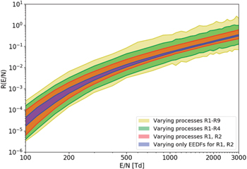
Figure 3. The uncertainty of the FNS/SPS ratio calculated by varying the kinetic data in the reduced model. With each band, a new source of uncertainty is introduced. The largest yellow band is the overall uncertainty of the model, when considering all the kinetic data available in literature.
Download figure:
Standard image High-resolution image4.2.2. Uncertainty in electron-impact cross-sections of R1 and R2
Subsequently, we varied the electron-impact cross-sections of the processes R1 and R2 within the full-range of data available in literature. From the red band in figure 3, it is apparent that this increases the uncertainty in the electric field distinctly. For the FNS/SPS ratio of 10−2 the electric field now lies anywhere in the range between 350 and 560 Td.
4.2.3. Uncertainty in radiative de-excitation lifetimes
When we start varying also the radiative de-excitation lifetimes R3–R4 within the range available in literature (in addition to the electron-impact data discussed above), the uncertainty of the model is further increased. For the FNS/SPS ratio of 10−2 is the confidence interval of the electric field 290–740 Td.
4.2.4. Uncertainty in quenching rate constants
Finally, when we also start varying the quenching rate constants R4-R9, there is a further dramatic increase in model uncertainty, as illustrated by the yellow band in figure 3. At the FNS/SPS ratio of 10−2, the predicted electric field now lies anywhere in the interval 230 and 880 Td. This is also the total uncertainty of the FNS/SPS model.
4.3. Comparison with R(E/N) curves in literature
In figure 4, we plot the total uncertainty band of the model together with theoretical R(E/N) curves obtained by other authors and one experimental. It is apparent that all the curves available in literature lie within the confidence band, as they should since the authors constructing these models worked with equivalent literature. This illustrates that the theoretical R(E/N) curve has very large uncertainty that has to be considered in data processing using this method. Considering that the electric field measured by the intensity ratio method might be further utilized for calculating the plasma kinetics and that electron-impact reactions often show exponential dependence on E/N, we can assert that reducing the R(E/N) uncertainty is very desirable.
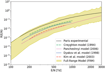
Figure 4. Comparison of the total confidence band of the FNS/SPS model with R(E/N) curves published in earlier works.
Download figure:
Standard image High-resolution imageSummarizing the results above, the differences among considered cross-section datasets present only a minor source of uncertainty of the theoretical R(E/N) curves.
On the other hand, the ionization and excitation cross-sections for the  and
and  states, as well as their quenching rates and radiative lifetimes all present substantial sources of uncertainty. Taking all of them into account, we find that the total uncertainty of the R(E/N) curves is very significant. The spread of R(E/N) curves available in literature confirms that there is no agreement in the community as to which kinetic data should be used for obtaining R(E/N).
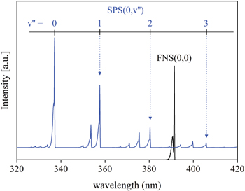
4.4. Spectrometric considerations
Figure 5 shows the synthetic spectra of SPS and FNS generated using models detailed in [1]. It should be underlined that in the case of FNS most of the emission originating from the v = 0 vibrational level goes indeed through the  transition, therefore the (0, 0) band of the FNS is the obvious choice for detection. However, in the case of the SPS emission, there are other options because several bands originating from the v = 0 level of the
  state occur with sufficient intensities, e.g. (0, 1), (0, 2) or (0, 3) bands indicated by arrows in the figure 5 at 357.7, 380.5 and 405.9 nm, respectively. Considering that the detection efficiency often increases from UV to visible spectral range, the combination of FNS(0, 0) and SPS(0, 2), or FNS(0, 0) and SPS(0, 3) might be better choice compared with the FNS(0, 0) and SPS(0, 0) case. This is certainly true in the case of remote spectrometric observation of transient luminous events because of heavy attenuation of the UV part of emission spectra, including the SPS(0, 0) band intensity. It is worth noting that Paris et al [5] also quantified the electric field dependence for the ratios of FNS(0, 0)/SPS(2, 5) and SPS(2, 5)/SPS(0, 0). The variation of the SPS(2, 5)/SPS(0, 0) intensity ratio in the low field region <300 Td is consistent with predicted E/N dependence of the rate constant for electron-impact excitation of individual vibration levels of the
  state [1]. A similar variation with the E/N should be obtained for other SPS bands, the (3, 6) and (1, 4) bands, occurring next or close to the FNS(0, 0) band (see figure 5). The FNS(0, 0)/SPS(3, 6) and FNS(0, 0)/SPS(1, 4) might provide alternative R(E/N) curves to be used simultaneously with R(E/N) curves derived from FNS(0, 0)/SPS(0, 3) and FNS(0, 0)/SPS(2, 5).
Figure 5. Synthetic emission spectra of the second positive system of N2 and (0, 0) band of the first negative system of N2
+. Calculated using triangular instrumental function and rotational temperature of 300 K. Spectrometric representation of the FCF-like vibrational distribution of the  state defined by Franck–Condon factors between (
 , v = 0–4) and (
 , v = 0) levels.
Download figure:
Standard image High-resolution image
Each of these ratios dependences represents a diagnostic tool for the determination of the reduced electric field. Each of these dependencies would require additional uncertainty quantification, which would also consider the uncertainty in the respective vibrational transitions and Frank–Condon factors. However, the 9 influential processes identified in this work are also valid for other FNS/SPS bands.
5. Conclusions
This work focuses on the intensity ratio method for the determination of the electric field in N2/O2 plasmas with the aim to evaluate the main sources of uncertainty in the R(E/N) curve and to quantify the total uncertainty of the method. Since the theoretical R(E/N) curve is obtained by solving the non-equilibrium kinetics in N2/O2 mixture, we first utilized sensitivity analysis according to Morris [24] to identify the key pathways leading to the population of the radiative N2 states, from which the FNS/SPS ratio is measured. The sensitivity analysis has revealed that 9 reactions are influential for the population and de-population of the  and
and  states. To be able to compare the sensitivity analysis to Townsend discharge-based experimental calibration curve by [5], we carried it out at the values of electron density and reduced electric field that are relevant to the Townsend discharge conditions. It is worth noting that these 9 processes have generally been considered important by the authors developing and improving the intensity ratio method. This work provides a sound mathematical justification for this choice. It also gives insight into the importance of three-body quenching which has been discussed in the community and which we have shown to only gain importance at low electric fields. Consequently, we varied the rate constants of these 9 most influential processes within the range of values available in literature. We arrived at the conclusion that the total uncertainty of the R(E/N) curve is as large as half an order of magnitude. By quantifying the uncertainty, we provide the community with the confidence interval for the R(E/N) curve. Knowing that the confidence band is very broad and knowing the processes which cause the uncertainty is a necessary starting point for reducing this uncertainty and obtaining a more accurate R(E/N). In part II to this publication, we take the first step in this direction, carefully revising the kinetic data available in literature and constructing a 'state-of-the-art model' with substantially reduced uncertainty of the R(E/N) curve. In a more general perspective, this work presents a suitable methodology for approaching plasma kinetics calculations. The goal of a complex plasma model is often to predict a single or a few quantities. By applying a method of sensitivity analysis, we isolate only those processes that are influential for the desired model output. Consequently, we quantify, how the uncertainty of the model inputs manifests in the overall uncertainty of the model predictions. Supplying the model prediction together with its uncertainty should be a best practice when comparing theoretical predictions to experimental results or to each other.
Acknowledgments
This work was supported by the Czech Science Foundation research project 15-04023S and partially support of project LO1411 (NPU I) funded by the Ministry of Education, Youth and Sports of the Czech Republic. ZB acknowledges discussions with Dr Nikolay A Popov concerning three-body quenching. Computational resources were supplied by the Ministry of Education, Youth and Sports of the Czech Republic under the Projects CESNET (Project No. LM2015042) and CERIT-Scientific Cloud (Project No. LM2015085) provided within the program Projects of Large Research, Development and Innovations Infrastructures.
: Appendix. Kinetic scheme
This appendix provides the full kinetic scheme as discussed in section 2.1. This kinetic scheme is based on works [25–28] as compiled in ZDPlasKin [29] library, input file for N2–O2 mixture (version 1.03). The following effective temperatures are used in the table A1 [134]. Note that Tgas is kept at 300 K within this work.
Table A1. Full kinetic scheme for air plasma.
| No. | Reaction | Rate coefficient |
|---|---|---|
| P001 | e + N2
 e + N2(A3, v = 0–4) e + N2(A3, v = 0–4) |

|
| P002 | e + N2
 e + N2(A3, v = 5–9) e + N2(A3, v = 5–9) |

|
| P003 | e + N2
 e + N2(A3, v>10) e + N2(A3, v>10) |

|
| P004 | e + N2
 e + N2(B3) e + N2(B3) |

|
| P005 | e + N2
 e + N2(W3) e + N2(W3) |

|
| P006 | e + N2
 e + N2(B'3) e + N2(B'3) | f(E/N) |
| P007 | e + N2
 e + N2(a'1) e + N2(a'1) | f(E/N) |
| P008 | e + N2
 e + N2(a1) e + N2(a1) | f(E/N) |
| P009 | e + N2
 e + N2(w1) e + N2(w1) | f(E/N) |
| P010 | e + N2
 e + N2(C3) e + N2(C3) | f(E/N) |
| P011 | e + N2
 e + N + N(2D) e + N + N(2D) | f(E/N) |
| P012 | e + O2
 e + O2(a1) e + O2(a1) | f(E/N) |
| P013 | e + O2
 e + O2(b1) e + O2(b1) | f(E/N) |
| P014 | e + O2
 e + O2(4.5 eV) e + O2(4.5 eV) | f(E/N) |
| P015 | e + O2
 e + O + O e + O + O | f(E/N) |
| P016 | e + O2
 e + O + O(1D) e + O + O(1D) | f(E/N) |
| P017 | e + O2
 e + O + O(1S) e + O + O(1S) | f(E/N) |
| P018 | e + O2(a1)  e + O + O e + O + O | f(E/N) |
| P019 | e + O  e + O(1D) e + O(1D) | f(E/N) |
| P020 | e + O  e + O(1S) e + O(1S) | f(E/N) |
| P021 | e + N  e + e + N+ e + e + N+
| f(E/N) |
| P022 | e + O  e + e + O+ e + e + O+
| f(E/N) |
| P023 | e + N2
 e + e + e + e + 
|

|
| P024 | e + N2(A3)  e + e + e + e + 
| f(E/N) |
| P025 | e + O2
 e + e + e + e + 
| f(E/N) |
| P026 | e + O2(a1)  e + e + e + e + 
| f(E/N) |
| P027 | e + NO  e + e + NO+ e + e + NO+
| f(E/N) |
| P028 | e + N2
 e + e + e + e + 
| f(E/N) |
| P029 | e + NO  e + e + e + e +  + O + O | f(E/N) |
| P030 | e + NO  e + e + N + O+ e + e + N + O+
| f(E/N) |
| P031 | e + N2O  e + e + N2O+ e + e + N2O+
| f(E/N) |
| P032 | e + 
 N + N N + N | 1.8e-7*(300.0/Te)**0.39*0.50 |
| P033 | e + 
 N + N(2D) N + N(2D) | 1.8e-7*(300.0/Te)**0.39*0.45 |
| P034 | e + 
 N + N(2P) N + N(2P) | 1.8e-7*(300.0/Te)**0.39*0.05 |
| P035 | e + 
 O + O O + O | 2.7e-7*(300.0/Te)**0.7*0.55 |
| P036 | e + 
 O + O(1D) O + O(1D) | 2.7e-7*(300.0/Te)**0.7*0.40 |
| P037 | e + 
 O + O(1S) O + O(1S) | 2.7e-7*(300.0/Te)**0.7*0.05 |
| P038 | e + NO+
 O + N O + N | 4.2e-7*(300.0/Te)**0.85*0.20 |
| P039 | e + NO+
 O + N(2D) O + N(2D) | 4.2e-7*(300.0/Te)**0.85*0.80 |
| P040 | e + 
 N2 + N N2 + N | 2.0e-7*(300.0/Te)**0.5 |
| P041 | e + 
 N2 + N2(C3) N2 + N2(C3) | 2.3e-6*(300.0/Te)**0.53 |
| P042 | e + N2O+
 N2 + O N2 + O | 2.0e-7*(300.0/Te)**0.5 |
| P043 | e + 
 NO + O NO + O | 2.0e-7*(300.0/Te)**0.5 |
| P044 | e + 
 O2 + O2 O2 + O2
| 1.4e-6*(300.0/Te)**0.5 |
| P045 | e +  N2 N2
 O2 + N2 O2 + N2
| 1.3e-6*(300.0/Te)**0.5 |
| P046 | e +  + e + e  N + e N + e | 7.0e-20*(300.0/Te)**4.5 |
| P047 | e +  + e + e  O + e O + e | 7.0e-20*(300.0/Te)**4.5 |
| P048 | e +  + M + M  N + M N + M | 6.0e-27*(300.0/Te)**1.5 |
| P049 | e +  + M + M  O + M O + M | 6.0e-27*(300.0/Te)**1.5 |
| P050 | e + 

 + e + e |

|
| P051 | e + O2

 + O + O |

|
| P052 | e + NO 
 + N + N |

|
| P053 | e + O3

 + O2 + O2
|

|
| P054 | e + O3

 + O + O |

|
| P055 | e + O2(a1)  O + O + 
|

|
| P056 | e + O2 + O2

 + O2 + O2
|

|
| P057 | e + NO2

 + NO + NO | 1.0e-11 |
| P058 | e + O + O2

 + O2 + O2
| 1.0e-31 |
| P059 | e + O + O2

 + O + O | 1.0e-31 |
| P060 | e + O3 + M 
 + M + M | 1.0e-31 |
| P061 | e + NO + M  NO− + M NO− + M | 8.0e-31 |
| P062 | e + N2O + M  N2O− + M N2O− + M | 6.0e-33 |
| P063 | e + O2 + N2

 +N2 +N2
| 1.1e-31*(300.0/Te)**2*exp(-70.0/Tgas)*exp(1 500.0*(Te-Tgas)/(Te*Tgas)) |
| P064 |
 + O + O  O2 + e O2 + e | 1.4e-10 |
| P065 |
 + N + N  NO + e NO + e | 2.6e-10 |
| P066 |
 + NO + NO  NO2 + e NO2 + e | 2.6e-10 |
| P067 |
 + N2 + N2
 N2O + e N2O + e | 5.0e-13 |
| P068 |
 + O2 + O2
 O3 + e O3 + e | 5.0e-15 |
| P069 |

 O3 + e O3 + e | 3.0e-10 |
| P070 |
 + O2(b1) + O2(b1)  O + O2 + e O + O2 + e | 6.9e-10 |
| P071 |
 + N2(A3) + N2(A3)  O + N2 + e O + N2 + e | 2.2e-9 |
| P072 |
 + N2(B3) + N2(B3)  O + N2 + e O + N2 + e | 1.9e-9 |
| P073 |
 + O3 + O3
 O2 + O2 + e O2 + O2 + e | 3.0e-10 |
| P074 |
 + O + O  O3 + e O3 + e | 1.5e-10 |
| P075 |
 + N + N  NO2 + e NO2 + e | 5.0e-10 |
| P076 |
 + O2 + O2
 O2 + O2 + e O2 + O2 + e | 2.7e-10*(TeffN2/300.0)**0.5*exp(-5 590.0/TeffN2) |
| P077 |
 + O2(a1) + O2(a1)  O2 + O2 + e O2 + O2 + e | 2.0e-10 |
| P078 |
 + O2(b1) + O2(b1)  O2 + O2 + e O2 + O2 + e | 3.6e-10 |
| P079 |
 + N2 + N2
 O2 + N2 + e O2 + N2 + e | 1.9e-12*(TeffN2/300.0)**0.5*exp(-4 990.0/TeffN2) |
| P080 |
 + N2(A3) + N2(A3)  O2 + N2 + e O2 + N2 + e | 2.1e-9 |
| P081 |
 + N2(B3) + N2(B3)  O2 + N2 + e O2 + N2 + e | 2.5e-9 |
| P082 |
 + O + O  O2 + O2 + e O2 + O2 + e | 3.0e-10 |
| P083 | NO− + N  N2O + e N2O + e | 5.0e-10 |
| P084 |
 + N + N  NO + O2 + e NO + O2 + e | 5.0e-10 |
| P085 | N2O− + N  NO + N2 + e NO + N2 + e | 5.0e-10 |
| P086 |
 + N + N  NO + NO + e NO + NO + e | 5.0e-10 |
| P087 |
 + N + N  NO + NO2 + e NO + NO2 + e | 5.0e-10 |
| P088 | NO− + O  NO2 + e NO2 + e | 1.5e-10 |
| P089 | N2O− + O  NO + NO + e NO + NO + e | 1.5e-10 |
| P090 |
 +O +O  NO + O2 + e NO + O2 + e | 1.5e-10 |
| P091 |
 + O + O  NO + O3 + e NO + O3 + e | 1.5e-10 |
| P092 |
 + N2(A3) + N2(A3)  O3 + N2 + e O3 + N2 + e | 2.1e-9 |
| P093 | NO− + N2(A3)  NO + N2 + e NO + N2 + e | 2.1e-9 |
| P094 | N2O− + N2(A3)  N2O + N2 + e N2O + N2 + e | 2.1e-9 |
| P095 |
 + N2(A3) + N2(A3)  NO2 + N2 + e NO2 + N2 + e | 2.1e-9 |
| P096 |
 + N2(A3) + N2(A3)  NO3 + N2 + e NO3 + N2 + e | 2.1e-9 |
| P097 |
 + N2(B3) + N2(B3)  O3 + N2 + e O3 + N2 + e | 2.5e-9 |
| P098 | NO− + N2(B3)  NO + N2 + e NO + N2 + e | 2.5e-9 |
| P099 | N2O− + N2(B3)  N2O + N2 + e N2O + N2 + e | 2.5e-9 |
| P100 |
 + N2(B3) + N2(B3)  NO2 + N2 + e NO2 + N2 + e | 2.5e-9 |
| P101 |
 + N2(B3) + N2(B3)  NO3 + N2 + e NO3 + N2 + e | 2.5e-9 |
| P102 | N2(A3)  N2 N2
| 0.50 |
| P103 | N2(B3)  N2(A3) N2(A3) | 1.34e5 |
| P104 | N2(a'1)  N2 N2
| 1.0e2 |
| P105 | N2(C3)  N2(B3) N2(B3) | 2.39e7 |
| P106 |


| 1.6e7 |
| P107 | O2(a1)  O2 O2
| 2.6e-4 |
| P108 | O2(b1)  O2(a1) O2(a1) | 1.5e-3 |
| P109 | O2(b1)  O2 O2
| 8.5e-2 |
| P110 | O2(4.5eV)  O2 O2
| 11.0 |
| P111 | N2(A3) + O  NO + N(2D) NO + N(2D) | 7.0e-12 |
| P112 | N2(A3) + O  N2 + O(1S) N2 + O(1S) | 2.1e-11 |
| P113 | N2(A3) + N  N2 + N N2 + N | 2.0e-12 |
| P114 | N2(A3) + N  N2 + N(2P) N2 + N(2P) | 4.0e-11*(300.0/Tgas)**0.667 |
| P115 | N2(A3) + O2
 N2 + O + O(1D) N2 + O + O(1D) | 2.1e-12*(Tgas/300.0)**0.55 |
| P116 | N2(A3) + O2
 N2 + O2(a1) N2 + O2(a1) | 2.0e-13*(Tgas/300.0)**0.55 |
| P117 | N2(A3) + O2
 N2 + O2(b1) N2 + O2(b1) | 2.0e-13*(Tgas/300.0)**0.55 |
| P118 | N2(A3) + O2
 N2O + O N2O + O | 2.0e-14*(Tgas/300.0)**0.55 |
| P119 | N2(A3) + N2
 N2 + N2 N2 + N2
| 3.0e-16 |
| P120 | N2(A3) + NO  N2+ NO N2+ NO | 6.9e-11 |
| P121 | N2(A3) + N2O  N2 + N + NO N2 + N + NO | 1.0e-11 |
| P122 | N2(A3) + NO2
 N2 + O + NO N2 + O + NO | 1.0e-12 |
| P123 | N2(A3) + N2(A3)  N2 + N2(B3) N2 + N2(B3) | 3.0e-10 |
| P124 | N2(A3) + N2(A3)  N2 + N2(C3) N2 + N2(C3) | 1.5e-10 |
| P125 | N2(B3) + N2
 N2(A3) + N2 N2(A3) + N2
| 3.0e-11 |
| P126 | N2(B3) + N2
 N2 + N2 N2 + N2
| 2.0e-12 |
| P127 | N2(B3) + O2
 N2 + O + O N2 + O + O | 3.0e-10 |
| P128 | N2(B3) + NO  N2(A3) + NO N2(A3) + NO | 2.4e-10 |
| P129 | N2(C3) + N2
 N2(a'1) + N2 N2(a'1) + N2
| 1.32e-11 |
| P130 | N2(C3) + O2
 N2 + O + O(1S) N2 + O + O(1S) | 2.9e-10 |
| P131 | N2(a'1) + N2
 N2(B3) + N2 N2(B3) + N2
| 1.9e-13 |
| P132 | N2(a'1) + O2
 N2 + O + O N2 + O + O | 2.8e-11 |
| P133 | N2(a'1) + NO  N2 + N + O N2 + N + O | 3.6e-10 |
| P134 | N2(a'1) + N2(A3) 
 + e + e | 4.0e-12 |
| P135 | N2(a'1) + N2(a'1) 
 + e + e | 1.0e-11 |
| P136 | N + N + N2
 N2(A3) + N2 N2(A3) + N2
| 1.7e-33 |
| P137 | N + N + O2
 N2(A3) + O2 N2(A3) + O2
| 1.7e-33 |
| P138 | N + N + NO  N2(A3) + NO N2(A3) + NO | 1.7e-33 |
| P139 | N + N + N  N2(A3) + N N2(A3) + N | 1.0e-32 |
| P140 | N + N + O  N2(A3) + O N2(A3) + O | 1.0e-32 |
| P141 | N + N + N2
 N2(B3) + N2 N2(B3) + N2
| 2.4e-33 |
| P142 | N + N + O2
 N2(B3) + O2 N2(B3) + O2
| 2.4e-33 |
| P143 | N + N + NO  N2(B3) + NO N2(B3) + NO | 2.4e-33 |
| P144 | N + N + N  N2(B3) + N N2(B3) + N | 1.4e-32 |
| P145 | N + N + O  N2(B3) + O N2(B3) + O | 1.4e-32 |
| P146 | N(2D) + O  N + O(1D) N + O(1D) | 4.0e-13 |
| P147 | N(2D) + O2
 NO + O NO + O | 5.2e-12 |
| P148 | N(2D) + NO  N2 + O N2 + O | 1.8e-10 |
| P149 | N(2D) + N2O  NO + N2 NO + N2
| 3.5e-12 |
| P150 | N(2D) + N2
 N + N2 N + N2
| 1.0e-13*exp(-510.0/Tgas) |
| P151 | N(2P) + N  N + N N + N | 1.8e-12 |
| P152 | N(2P) + O  N + O N + O | 1.0e-12 |
| P153 | N(2P) + N  N(2D) + N N(2D) + N | 6.0e-13 |
| P154 | N(2P) + N2
 N + N2 N + N2
| 6.0e-14 |
| P155 | N(2P) + N(2D) 
 + e + e | 1.0e-13 |
| P156 | N(2P) + O2
 NO + O NO + O | 2.6e-12 |
| P157 | N(2P) + NO  N2(A3) + O N2(A3) + O | 3.0e-11 |
| P158 | O2(a1) + O  O2 + O O2 + O | 7.0e-16 |
| P159 | O2(a1) + N  NO + O NO + O | 2.0e-14*exp(-600.0/Tgas) |
| P160 | O2(a1) + O2
 O2 + O2 O2 + O2
| 3.8e-18*exp(-205.0/Tgas) |
| P161 | O2(a1) + N2
 O2 + N2 O2 + N2
| 3.0e-21 |
| P162 | O2(a1) + NO  O2 + NO O2 + NO | 2.5e-11 |
| P163 | O2(a1) + O3
 O2 + O2 + O(1D) O2 + O2 + O(1D) | 5.2e-11*exp(-2 840.0/Tgas) |
| P164 | O2(a1) + O2(a1)  O2 + O2(b1) O2 + O2(b1) | 7.0e-28*Tgas**3.8*exp(700.0/Tgas) |
| P165 | O + O3
 O2 + O2(a1) O2 + O2(a1) | 1.0e-11*exp(-2 300.0/Tgas) |
| P166 | O2(b1) + O  O2(a1) + O O2(a1) + O | 8.1e-14 |
| P167 | O2(b1) + O  O2 + O(1D) O2 + O(1D) | 3.4e-11*(300.0/Tgas)**0.1*exp(-4 200.0/Tgas) |
| P168 | O2(b1) + O2
 O2(a1) + O2 O2(a1) + O2
| 4.3e-22*Tgas**2.4*exp(-281.0/Tgas) |
| P169 | O2(b1) + N2
 O2(a1) + N2 O2(a1) + N2
| 1.7e-15*(Tgas/300.0) |
| P170 | O2(b1) + NO  O2(a1) + NO O2(a1) + NO | 6.0e-14 |
| P171 | O2(b1) + O3
 O2 + O2 + O O2 + O2 + O | 2.2e-11 |
| P172 | O2(4.5 eV) + O  O2 + O(1S) O2 + O(1S) | 9.0e-12 |
| P173 | O2(4.5 eV) + O2
 O2(b1) + O2(b1) O2(b1) + O2(b1) | 3.0e-13 |
| P174 | O2(4.5 eV) + N2
 O2(b1) + N2 O2(b1) + N2
| 9.0e-15 |
| P175 | O(1D) + O  O + O O + O | 8.0e-12 |
| P176 | O(1D) + O2
 O + O2 O + O2
| 6.4e-12*exp(67.0/Tgas) |
| P177 | O(1D) + O2
 O + O2(a1) O + O2(a1) | 1.0e-12 |
| P178 | O(1D) + O2
 O + O2(b1) O + O2(b1) | 2.6e-11*exp(67.0/Tgas) |
| P179 | O(1D) + N2
 O + N2 O + N2
| 2.3e-11 |
| P180 | O(1D) + O3
 O2 + O + O O2 + O + O | 1.2e-10 |
| P181 | O(1D) + O3
 O2 + O2 O2 + O2
| 1.2e-10 |
| P182 | O(1D) + NO  O2 + N O2 + N | 1.7e-10 |
| P183 | O(1D) + N2O  NO + NO NO + NO | 7.2e-11 |
| P184 | O(1D) + N2O  O2 + N2 O2 + N2
| 4.4e-11 |
| P185 | O(1S) + O  O(1D) + O O(1D) + O | 5.0e-11*exp(-300.0/Tgas) |
| P186 | O(1S) + N  O + N O + N | 1.0e-12 |
| P187 | O(1S) + O2
 O(1D) + O2 O(1D) + O2
| 1.3e-12*exp(-850.0/Tgas) |
| P188 | O(1S) + O2
 O + O + O O + O + O | 3.0e-12*exp(-850.0/Tgas) |
| P189 | O(1S) + N2
 O + N2 O + N2
| 1.0e-17 |
| P190 | O(1S) + O2(a1)  O + O2(4.5 eV) O + O2(4.5 eV) | 1.1e-10 |
| P191 | O(1S) + O2(a1)  O(1D) + O2(b1) O(1D) + O2(b1) | 2.9e-11 |
| P192 | O(1S) + O2(a1)  O + O + O O + O + O | 3.2e-11 |
| P193 | O(1S) + NO  O + NO O + NO | 2.9e-10 |
| P194 | O(1S) + NO  O(1D) + NO O(1D) + NO | 5.1e-10 |
| P195 | O(1S) + O3
 O2 + O2 O2 + O2
| 2.9e-10 |
| P196 | O(1S) + O3
 O2 + O + O(1D) O2 + O + O(1D) | 2.9e-10 |
| P197 | O(1S) + N2O  O + N2O O + N2O | 6.3e-12 |
| P198 | O(1S) + N2O  O(1D) + N2O O(1D) + N2O | 3.1e-12 |
| P199 | N + NO  O + N2 O + N2
| 1.8e-11*(Tgas/300.0)**0.5 |
| P200 | N + O2
 O + NO O + NO | 3.2e-12*(Tgas/300.0)*exp(-3 150.0/Tgas) |
| P201 | N + NO2
 O + O + N2 O + O + N2
| 9.1e-13 |
| P202 | N + NO2
 O + N2O O + N2O | 3.0e-12 |
| P203 | N + NO2
 N2 + O2 N2 + O2
| 7.0e-13 |
| P204 | N + NO2
 NO + NO NO + NO | 2.3e-12 |
| P205 | O + N2
 N + NO N + NO | 3.0e-10*exp(-38 370.0/Tgas) |
| P206 | O + NO  N + O2 N + O2
| 7.5e-12*(Tgas/300.0)*exp(-19 500.0/Tgas) |
| P207 | O + NO  NO2 NO2
| 4.2e-18 |
| P208 | O + N2O  N2 + O2 N2 + O2
| 8.3e-12*exp(-14 000.0/Tgas) |
| P209 | O + N2O  NO + NO NO + NO | 1.5e-10*exp(-14 090.0/Tgas) |
| P210 | O + NO2
 NO + O2 NO + O2
| 9.1e-12*(Tgas/300.0)**0.18 |
| P211 | O + NO3
 O2 + NO2 O2 + NO2
| 1.0e-11 |
| P212 | N2 + O2
 O + N2O O + N2O | 2.5e-10*exp(-50 390.0/Tgas) |
| P213 | NO + NO  N + NO2 N + NO2
| 3.3e-16*(300.0/Tgas)**0.5*exp(-39 200.0/Tgas) |
| P214 | NO + NO  O + N2O O + N2O | 2.2e-12*exp(-32 100.0/Tgas) |
| P215 | NO + NO  N2 + O2 N2 + O2
| 5.1e-13*exp(-33 660.0/Tgas) |
| P216 | NO + O2
 O + NO2 O + NO2
| 2.8e-12*exp(-23 400.0/Tgas) |
| P217 | NO + O3
 O2 + NO2 O2 + NO2
| 2.5e-13*exp(-765.0/Tgas) |
| P218 | NO + N2O  N2 + NO2 N2 + NO2
| 4.6e-10*exp(-25 170.0/Tgas) |
| P219 | NO + NO3
 NO2 + NO2 NO2 + NO2
| 1.7e-11 |
| P220 | O2 + O2
 O + O3 O + O3
| 2.0e-11*exp(-49 800.0/Tgas) |
| P221 | O2 + NO2
 NO + O3 NO + O3
| 2.8e-12*exp(-25 400.0/Tgas) |
| P222 | NO2 + NO2
 NO + NO + O2 NO + NO + O2
| 3.3e-12*exp(-13 500.0/Tgas) |
| P223 | NO2 + NO2
 NO + NO3 NO + NO3
| 4.5e-10*exp(-18 500.0/Tgas) |
| P224 | NO2 + O3
 O2 + NO3 O2 + NO3
| 1.2e-13*exp(-2 450.0/Tgas) |
| P225 | NO2 + NO3
 NO + NO2 + O2 NO + NO2 + O2
| 2.3e-13*exp(-1 600.0/Tgas) |
| P226 | NO3 + O2
 NO2 + O3 NO2 + O3
| 1.5e-12*exp(-15 020.0/Tgas) |
| P227 | NO3 + NO3
 O2 + NO2 + NO2 O2 + NO2 + NO2
| 4.3e-12*exp(-3 850.0/Tgas) |
| P228 | N + N 
 + e + e | 2.7e-11*exp(-6.74e4/Tgas) |
| P229 | N + O  NO+ + e NO+ + e | 1.6e-12*(Tgas/300.0)**0.5*(0.19+8.6*Tgas)*exp(-32 000.0/Tgas) |
| P230 | N2 + N2
 N + N + N2 N + N + N2
| 5.4e-8*(1.0-exp(-3 354.0/Tgas))*exp(-113 200.0/Tgas)*1.0 |
| P231 | N2 + O2
 N + N + O2 N + N + O2
| 5.4e-8*(1.0-exp(-3 354.0/Tgas))*exp(-113 200.0/Tgas)*1.0 |
| P232 | N2 + NO  N + N + NO N + N + NO | 5.4e-8*(1.0-exp(-3 354.0/Tgas))*exp(-113 200.0/Tgas)*1.0 |
| P233 | N2 + O  N + N + O N + N + O | 5.4e-8*(1.0-exp(-3 354.0/Tgas))*exp(-113 200.0/Tgas)*6.6 |
| P234 | N2 + N  N + N + N N + N + N | 5.4e-8*(1.0-exp(-3 354.0/Tgas))*exp(-113 200.0/Tgas)*6.6 |
| P235 | O2 + N2
 O + O + N2 O + O + N2
| 6.1e-9*(1.0-exp(-2 240.0/Tgas))*exp(-59 380.0/Tgas)*1.0 |
| P236 | O2 + O2
 O + O + O2 O + O + O2
| 6.1e-9*(1.0-exp(-2 240.0/Tgas))*exp(-59 380.0/Tgas)*5.9 |
| P237 | O2 + O  O + O + O O + O + O | 6.1e-9*(1.0-exp(-2 240.0/Tgas))*exp(-59 380.0/Tgas)*21. |
| P238 | O2 + N  O + O + N O + O + N | 6.1e-9*(1.0-exp(-2 240.0/Tgas))*exp(-59 380.0/Tgas)*1.0 |
| P239 | O2 + NO  O + O + NO O + O + NO | 6.1e-9*(1.0-exp(-2 240.0/Tgas))*exp(-59 380.0/Tgas)*1.0 |
| P240 | NO + N2
 N + O + N2 N + O + N2
| 8.7e-9*exp(-75 994.0/Tgas)*1.0 |
| P241 | NO + O2
 N + O + O2 N + O + O2
| 8.7e-9*exp(-75 994.0/Tgas)*1.0 |
| P242 | NO + O  N + O + O N + O + O | 8.7e-9*exp(-75 994.0/Tgas)*20. |
| P243 | NO + N  N + O + N N + O + N | 8.7e-9*exp(-75 994.0/Tgas)*20. |
| P244 | NO + NO  N + O + NO N + O + NO | 8.7e-9*exp(-75 994.0/Tgas)*20. |
| P245 | O3 + N2
 O2 + O + N2 O2 + O + N2
| 6.6e-10*exp(-11 600.0/Tgas)*1.0 |
| P246 | O3 + O2
 O2 + O + O2 O2 + O + O2
| 6.6e-10*exp(-11 600.0/Tgas)*0.38 |
| P247 | O3 + N  O2 + O + N O2 + O + N | 6.6e-10*exp(-11 600.0/Tgas)*6.3*exp(170.0/Tgas) |
| P248 | O3 + O  O2 + O + O O2 + O + O | 6.6e-10*exp(-11 600.0/Tgas)*6.3*exp(170.0/Tgas) |
| P249 | N2O + N2
 N2 + O + N2 N2 + O + N2
| 1.2e-8*(300.0/Tgas)*exp(-29 000.0/Tgas)*1.0 |
| P250 | N2O + O2
 N2 + O + O2 N2 + O + O2
| 1.2e-8*(300.0/Tgas)*exp(-29 000.0/Tgas)*1.0 |
| P251 | N2O + NO  N2 + O + NO N2 + O + NO | 1.2e-8*(300.0/Tgas)*exp(-29 000.0/Tgas)*2.0 |
| P252 | N2O + N2O  N2 + O + N2O N2 + O + N2O | 1.2e-8*(300.0/Tgas)*exp(-29 000.0/Tgas)*4.0 |
| P253 | NO2 + N2
 NO + O + N2 NO + O + N2
| 6.8e-6*(300.0/Tgas)**2*exp(-36 180.0/Tgas)*1.0 |
| P254 | NO2 + O2
 NO + O + O2 NO + O + O2
| 6.8e-6*(300.0/Tgas)**2*exp(-36 180.0/Tgas)*0.78 |
| P255 | NO2 + NO  NO + O + NO NO + O + NO | 6.8e-6*(300.0/Tgas)**2*exp(-36 180.0/Tgas)*7.8 |
| P256 | NO2 + NO2
 NO + O + NO2 NO + O + NO2
| 6.8e-6*(300.0/Tgas)**2*exp(-36 180.0/Tgas)*5.9 |
| P257 | NO3 + N2
 NO2 + O + N2 NO2 + O + N2
| 3.1e-5*(300.0/Tgas)**2*exp(-25 000.0/Tgas)*1.0 |
| P258 | NO3 + O2
 NO2 + O + O2 NO2 + O + O2
| 3.1e-5*(300.0/Tgas)**2*exp(-25 000.0/Tgas)*1.0 |
| P259 | NO3 + NO  NO2 + O + NO NO2 + O + NO | 3.1e-5*(300.0/Tgas)**2*exp(-25 000.0/Tgas)*1.0 |
| P260 | NO3 + N  NO2 + O + N NO2 + O + N | 3.1e-5*(300.0/Tgas)**2*exp(-25 000.0/Tgas)*10. |
| P261 | NO3 + O  NO2 + O + O NO2 + O + O | 3.1e-5*(300.0/Tgas)**2*exp(-25 000.0/Tgas)*10. |
| P262 | NO3 + N2
 NO + O2 + N2 NO + O2 + N2
| 6.2e-5*(300.0/Tgas)**2*exp(-25 000.0/Tgas)*1.0 |
| P263 | NO3 + O2
 NO + O2 + O2 NO + O2 + O2
| 6.2e-5*(300.0/Tgas)**2*exp(-25 000.0/Tgas)*1.0 |
| P264 | NO3 + NO  NO + O2 + NO NO + O2 + NO | 6.2e-5*(300.0/Tgas)**2*exp(-25 000.0/Tgas)*1.0 |
| P265 | NO3 + N  NO + O2 + N NO + O2 + N | 6.2e-5*(300.0/Tgas)**2*exp(-25 000.0/Tgas)*12. |
| P266 | NO3 + O  NO + O2 + O NO + O2 + O | 6.2e-5*(300.0/Tgas)**2*exp(-25 000.0/Tgas)*12. |
| P267 | N2O5 + M  NO2 + NO3 + M NO2 + NO3 + M | 2.1e-11*(300.0/Tgas)**4.4*exp(-11 080.0/Tgas) |
| P268 | N + N + N2
 N2 + N2 N2 + N2
| max(8.3e-34*exp(500.0/Tgas) , 1.91e-33 ) |
| P269 | N + N + O2
 N2 + O2 N2 + O2
| 1.8e-33*exp(435.0/Tgas)*1.0 |
| P270 | N + N + NO  N2 + NO N2 + NO | 1.8e-33*exp(435.0/Tgas)*1.0 |
| P271 | N + N + N  N2 + N N2 + N | 1.8e-33*exp(435.0/Tgas)*3.0 |
| P272 | N + N + O  N2 + O N2 + O | 1.8e-33*exp(435.0/Tgas)*3.0 |
| P273 | O + O + N2
 O2 + N2 O2 + N2
| max(2.8e-34*exp(720.0/Tgas) , 1.0e-33*(300.0/Tgas)**0.41 ) |
| P274 | O + O + O2
 O2 + O2 O2 + O2
| 4.0e-33*(300.0/Tgas)**0.41*1.0 |
| P275 | O + O + N  O2 + N O2 + N | 4.0e-33*(300.0/Tgas)**0.41*0.8 |
| P276 | O + O + O  O2 + O O2 + O | 4.0e-33*(300.0/Tgas)**0.41*3.6 |
| P277 | O + O + NO  O2 + NO O2 + NO | 4.0e-33*(300.0/Tgas)**0.41*0.17 |
| P278 | N + O + N2
 NO + N2 NO + N2
| 1.0e-32*(300.0/Tgas)**0.5 |
| P279 | N + O + O2
 NO + O2 NO + O2
| 1.0e-32*(300.0/Tgas)**0.5 |
| P280 | N + O + N  NO + N NO + N | 1.8e-31*(300.0/Tgas) |
| P281 | N + O + O  NO + O NO + O | 1.8e-31*(300.0/Tgas) |
| P282 | N + O + NO  NO + NO NO + NO | 1.8e-31*(300.0/Tgas) |
| P283 | O + O2 + N2
 O3 + N2 O3 + N2
| max(5.8e-34*(300.0/Tgas)**2.8 , 5.4e-34*(300.0/Tgas)**1.9 ) |
| P284 | O + O2 + O2
 O3 + O2 O3 + O2
| 7.6e-34*(300.0/Tgas)**1.9 |
| P285 | O + O2 + NO  O3 + NO O3 + NO | 7.6e-34*(300.0/Tgas)**1.9 |
| P286 | O + O2 + N  O3 + N O3 + N | min(3.9e-33*(300.0/Tgas)**1.9 , 1.1e-34*exp(1 060.0/Tgas) ) |
| P287 | O + O2 + O  O3 + O O3 + O | min(3.9e-33*(300.0/Tgas)**1.9 , 1.1e-34*exp(1 060.0/Tgas) ) |
| P288 | O + N2 + M  N2O + M N2O + M | 3.9e-35*exp(-10 400.0/Tgas) |
| P289 | O + NO + N2
 NO2 + N2 NO2 + N2
| 1.2e-31*(300.0/Tgas)**1.8*1.0 |
| P290 | O + NO + O2
 NO2 + O2 NO2 + O2
| 1.2e-31*(300.0/Tgas)**1.8*0.78 |
| P291 | O + NO + NO  NO2 + NO NO2 + NO | 1.2e-31*(300.0/Tgas)**1.8*0.78 |
| P292 | O + NO2 + N2
 NO3 + N2 NO3 + N2
| 8.9e-32*(300.0/Tgas)**2*1.0 |
| P293 | O + NO2 + O2
 NO3 + O2 NO3 + O2
| 8.9e-32*(300.0/Tgas)**2*1.0 |
| P294 | O + NO2 + N  NO3 + N NO3 + N | 8.9e-32*(300.0/Tgas)**2*13. |
| P295 | O + NO2 + O  NO3 + O NO3 + O | 8.9e-32*(300.0/Tgas)**2*13. |
| P296 | O + NO2 + NO  NO3 + NO NO3 + NO | 8.9e-32*(300.0/Tgas)**2*2.4 |
| P297 | NO2 + NO3 + M  N2O5 + M N2O5 + M | 3.7e-30*(300.0/Tgas)**4.1 |
| P298 |
 + O + O  N + N + 
| 1.0e-12 |
| P299 |
 + O2 + O2

 + N + N | 2.8e-10 |
| P300 |
 + O2 + O2
 NO+ + O NO+ + O | 2.5e-10 |
| P301 |
 + O2 + O2

 + NO + NO | 2.8e-11 |
| P302 |
 + O3 + O3
 NO+ + O2 NO+ + O2
| 5.0e-10 |
| P303 |
 + NO + NO  NO+ + N NO+ + N | 8.0e-10 |
| P304 |
 + NO + NO 
 + O + O | 3.0e-12 |
| P305 |
 + NO + NO 

| 1.0e-12 |
| P306 |
 O O  NO+ + N2 NO+ + N2
| 5.5e-10 |
| P307 |

 NO+ + N NO+ + N | (1.5-2.0e-3*TeffN + 9.6e-7*TeffN**2 )*1.0e-12 |
| P308 |
 + O2 + O2

 + O + O | 2.0e-11*(300.0/TeffN)**0.5 |
| P309 |
 + O3 + O3

 + O2 + O2
| 1.0e-10 |
| P310 |
 + NO + NO  NO+ + O NO+ + O | 2.4e-11 |
| P311 |
 + NO + NO 
 + N + N | 3.0e-12 |
| P312 |
 + N(2D) + N(2D) 
 + O + O | 1.3e-10 |
| P313 |
 O O  NO+ + NO NO+ + NO | 2.3e-10 |
| P314 |
 O O  N2O+ + O N2O+ + O | 2.2e-10 |
| P315 |
 O O 

| 2.0e-11 |
| P316 |
 + NO2 + NO2

 + O + O | 1.6e-9 |
| P317 |
 + O2 + O2


| 6.0e-11*(300.0/TeffN2)**0.5 |
| P318 |
 + O + O  NO+ + N NO+ + N | 1.3e-10*(300.0/TeffN2)**0.5 |
| P319 |
 + O3 + O3

 + O + N2 + O + N2
| 1.0e-10 |
| P320 |
 + N + N 

| 7.2e-13*(TeffN2/300.0) |
| P321 |
 + NO + NO  NO+ + N2 NO+ + N2
| 3.3e-10 |
| P322 |
 O O  N2O+ + N2 N2O+ + N2
| 5.0e-10 |
| P323 |
 O O  NO+ + N + N2 NO+ + N + N2
| 4.0e-10 |
| P324 |
 + O2 + O2


| 6.0e-11*(300.0/TeffN2)**0.5 |
| P325 |
 + O + O  NO+ + N NO+ + N | 1.3e-10*(300.0/TeffN2)**0.5 |
| P326 |
 + O3 + O3

 + O + N2 + O + N2
| 1.0e-10 |
| P327 |
 + N + N 

| 7.2e-13*(TeffN2/300.0) |
| P328 |
 + NO + NO  NO+ + N2 NO+ + N2
| 3.3e-10 |
| P329 |
 O O  N2O+ + N2 N2O+ + N2
| 5.0e-10 |
| P330 |
 O O  NO+ + N + N2 NO+ + N + N2
| 4.0e-10 |
| P331 |


| 8.8e-10 |
| P332 |
 + O2 + O2

 + O + O(1S) + O + O(1S) | 1.0e-9 |
| P333 |

 NO+ + NO NO+ + NO | 1.0e-17 |
| P334 |
 + N + N  NO+ + O NO+ + O | 1.2e-10 |
| P335 |
 + NO + NO  NO+ + O2 NO+ + O2
| 6.3e-10 |
| P336 |
 + NO2 + NO2
 NO+ + O3 NO+ + O3
| 1.0e-11 |
| P337 |
 + NO2 + NO2

 + O2 + O2
| 6.6e-10 |
| P338 |
 + O2 + O2

 + N + N2 + N + N2
| 2.3e-11 |
| P339 |
 + O2 + O2

 + N2 + N2
| 4.4e-11 |
| P340 |
 + N + N 

| 6.6e-11 |
| P341 |
 + NO + NO  NO+ + N + N2 NO+ + N + N2
| 7.0e-11 |
| P342 |
 + NO + NO  N2O+ + N2 N2O+ + N2
| 7.0e-11 |
| P343 |
 + NO + NO  NO+ + NO2 NO+ + NO2
| 2.9e-10 |
| P344 | N2O+ + NO  NO+ + N2O NO+ + N2O | 2.9e-10 |
| P345 |


| min(2.1e-16*exp(TeffN4/121.0), 1.0e-10 ) |
| P346 |
 + O2 + O2


| 2.5e-10 |
| P347 |
 + O + O 

| 2.5e-10 |
| P348 |
 + N + N 

| 1.0e-11 |
| P349 |
 + NO + NO  NO+ + N2 + N2 NO+ + N2 + N2
| 4.0e-10 |
| P350 |


 N2 + O2 N2 + O2
| 4.6e-12*(TeffN4/300.0)**2.5*exp(-2 650.0/TeffN4) |
| P351 |
 + O2 + O2

 + O2 + O2 + O2 + O2
| 3.3e-6 *(300.0/TeffN4)**4 *exp(-5 030.0/TeffN4) |
| P352 |
 + O2(a1) + O2(a1) 
 + O2 + O2 + O2 + O2
| 1.0e-10 |
| P353 |
 +O2(b1) +O2(b1) 
 + O2 + O2 + O2 + O2
| 1.0e-10 |
| P354 |
 + O + O 
 + O3 + O3
| 3.0e-10 |
| P355 |
 + NO + NO  NO+ + O2 + O2 NO+ + O2 + O2
| 1.0e-10 |
| P356 |
 N2 + N2 N2 + N2


| 1.1e-6*(300.0/TeffN4)**5.3*exp(-2 360.0/TeffN4) |
| P357 |
 N2 + O2 N2 + O2


| 1.0e-9 |
| P358 |


| 1.7e-29*(300.0/TeffN)**2.1 |
| P359 |
 + O + M + O + M  NO+ + M NO+ + M | 1.0e-29 |
| P360 |
 + N + M + N + M 
 + M + M | 1.0e-29 |
| P361 |
 + M + M  NO+ + N + M NO+ + N + M | 6.0e-29*(300.0/TeffN)**2 |
| P362 |
 + O + M + O + M 
 + M + M | 1.0e-29 |
| P363 |
 + N + M + N + M  NO+ + M NO+ + M | 1.0e-29 |
| P364 |


| 5.2e-29*(300.0/TeffN2)**2.2 |
| P365 |


| 9.0e-30*exp(400.0/TeffN2) |
| P366 |


| 6.2e-29*(300.0/Teff3Q)**1.7 |
| P367 |


| 9.0e-30*exp(400.0/TeffN2) |
| P368 |
 + O2 + O2 + O2 + O2

 + O2 + O2
| 2.4e-30*(300.0/TeffN2)**3.2 |
| P369 |


 N2 + N2 N2 + N2
| 9.0e-31*(300.0/TeffN2)**2 |
| P370 |


 + O + O | 1.0e-10 |
| P371 |
 + O3 + O3

 + O + O | 8.0e-10 |
| P372 |
 + NO2 + NO2

 + O + O | 1.2e-9 |
| P373 |
 + N2O + N2O  NO− + NO NO− + NO | 2.0e-10 |
| P374 |
 + N2O + N2O  N2O− + O N2O− + O | 2.0e-12 |
| P375 |
 + O + O 
 + O2 + O2
| 3.3e-10 |
| P376 |
 + O3 + O3

 + O2 + O2
| 3.5e-10 |
| P377 |
 + NO2 + NO2

 + O2 + O2
| 7.0e-10 |
| P378 |
 + NO3 + NO3

 + O2 + O2
| 5.0e-10 |
| P379 |
 + O + O 
 + O2 + O2
| 1.0e-11 |
| P380 |
 + NO + NO 
 + O + O | 1.0e-11 |
| P381 |
 + NO + NO 
 + O2 + O2
| 2.6e-12 |
| P382 |
 + NO2 + NO2

 + O3 + O3
| 7.0e-11 |
| P383 |
 + NO2 + NO2

 + O2 + O2
| 2.0e-11 |
| P384 |
 + NO3 + NO3

 + O3 + O3
| 5.0e-10 |
| P385 | NO− + O2

 + NO + NO | 5.0e-10 |
| P386 | NO− + NO2

 + NO + NO | 7.4e-10 |
| P387 | NO− + N2O 
 + N2 + N2
| 2.8e-14 |
| P388 |
 + O3 + O3

 + O2 + O2
| 1.8e-11 |
| P389 |
 + NO2 + NO2

 + NO + NO | 4.0e-12 |
| P390 |
 + NO3 + NO3

 + NO2 + NO2
| 5.0e-10 |
| P391 |
 + N2O5 + N2O5

 + NO2 + NO2 + NO2 + NO2
| 7.0e-10 |
| P392 |
 + NO + NO 
 + NO2 + NO2
| 3.0e-15 |
| P393 |
 + N2 + N2

 + O2 + N2 + O2 + N2
| 1.0e-10*exp(-1 044.0/TeffN4) |
| P394 |
 + O2 + O2

 + O2 + O2 + O2 + O2
| 1.0e-10*exp(-1 044.0/TeffN4) |
| P395 |
 + O + O 
 + O2 + O2
| 4.0e-10 |
| P396 |
 + O + O 
 + O2 + O2 + O2 + O2
| 3.0e-10 |
| P397 |
 + O2(a1) + O2(a1) 
 + O2 + O2 + O2 + O2
| 1.0e-10 |
| P398 |
 + O2(b1) + O2(b1) 
 + O2 + O2 + O2 + O2
| 1.0e-10 |
| P399 |
 + NO + NO 
 + O2 + O2
| 2.5e-10 |
| P400 |
 + O2 + M + O2 + M 
 + M + M | 1.1e-30*(300.0/TeffN) |
| P401 |
 + NO + M + NO + M 
 + M + M | 1.0e-29 |
| P402 |
 + O2 + M + O2 + M 
 + M + M | 3.5e-31*(300.0/TeffN2) |
| P403 |
 + + 
 O + N O + N | 2.0e-7*(300.0/TionN)**0.5 |
| P404 |
 + + 
 O + N2 O + N2
| 2.0e-7*(300.0/TionN)**0.5 |
| P405 |
 + + 
 O + O O + O | 2.0e-7*(300.0/TionN)**0.5 |
| P406 |
 + + 
 O + O2 O + O2
| 2.0e-7*(300.0/TionN)**0.5 |
| P407 |
 + NO+ + NO+
 O + NO O + NO | 2.0e-7*(300.0/TionN)**0.5 |
| P408 |
 + N2O+ + N2O+
 O + N2O O + N2O | 2.0e-7*(300.0/TionN)**0.5 |
| P409 |
 + + 
 O + NO2 O + NO2
| 2.0e-7*(300.0/TionN)**0.5 |
| P410 |
 + + 
 O + N2 O + N2
| 2.0e-7*(300.0/TionN)**0.5 |
| P411 |
 + + 
 O2 + N O2 + N | 2.0e-7*(300.0/TionN)**0.5 |
| P412 |
 + + 
 O2 + N2 O2 + N2
| 2.0e-7*(300.0/TionN)**0.5 |
| P413 |
 + + 
 O2 + O O2 + O | 2.0e-7*(300.0/TionN)**0.5 |
| P414 |
 + + 
 O2 + O2 O2 + O2
| 2.0e-7*(300.0/TionN)**0.5 |
| P415 |
 + NO+ + NO+
 O2 + NO O2 + NO | 2.0e-7*(300.0/TionN)**0.5 |
| P416 |
 + N2O+ + N2O+
 O2 + N2O O2 + N2O | 2.0e-7*(300.0/TionN)**0.5 |
| P417 |
 + + 
 O2 + NO2 O2 + NO2
| 2.0e-7*(300.0/TionN)**0.5 |
| P418 |
 + + 
 O2 + N2 O2 + N2
| 2.0e-7*(300.0/TionN)**0.5 |
| P419 |
 + + 
 O3 + N O3 + N | 2.0e-7*(300.0/TionN)**0.5 |
| P420 |
 + + 
 O3 + N2 O3 + N2
| 2.0e-7*(300.0/TionN)**0.5 |
| P421 |
 + + 
 O3 + O O3 + O | 2.0e-7*(300.0/TionN)**0.5 |
| P422 |
 + + 
 O3 + O2 O3 + O2
| 2.0e-7*(300.0/TionN)**0.5 |
| P423 |
 + NO+ + NO+
 O3 + NO O3 + NO | 2.0e-7*(300.0/TionN)**0.5 |
| P424 |
 + N2O+ + N2O+
 O3 + N2O O3 + N2O | 2.0e-7*(300.0/TionN)**0.5 |
| P425 |
 + + 
 O3 + NO2 O3 + NO2
| 2.0e-7*(300.0/TionN)**0.5 |
| P426 |
 + + 
 O3 + N2 O3 + N2
| 2.0e-7*(300.0/TionN)**0.5 |
| P427 | NO− + 
 NO + N NO + N | 2.0e-7*(300.0/TionN)**0.5 |
| P428 | NO− + 
 NO + N2 NO + N2
| 2.0e-7*(300.0/TionN)**0.5 |
| P429 | NO− + 
 NO + O NO + O | 2.0e-7*(300.0/TionN)**0.5 |
| P430 | NO− + 
 NO + O2 NO + O2
| 2.0e-7*(300.0/TionN)**0.5 |
| P431 | NO− + NO+
 NO + NO NO + NO | 2.0e-7*(300.0/TionN)**0.5 |
| P432 | NO− + N2O+
 NO + N2O NO + N2O | 2.0e-7*(300.0/TionN)**0.5 |
| P433 | NO− + 
 NO + NO2 NO + NO2
| 2.0e-7*(300.0/TionN)**0.5 |
| P434 | NO− + 
 NO + N2 NO + N2
| 2.0e-7*(300.0/TionN)**0.5 |
| P435 | NO− + 
 NO + N NO + N | 2.0e-7*(300.0/TionN)**0.5 |
| P436 | NO− + 
 NO + N2 NO + N2
| 2.0e-7*(300.0/TionN)**0.5 |
| P437 | NO− + 
 NO + O NO + O | 2.0e-7*(300.0/TionN)**0.5 |
| P438 | NO− + 
 NO + O2 NO + O2
| 2.0e-7*(300.0/TionN)**0.5 |
| P439 | NO− + NO+
 NO + NO NO + NO | 2.0e-7*(300.0/TionN)**0.5 |
| P440 | NO− + N2O+
 NO + N2O NO + N2O | 2.0e-7*(300.0/TionN)**0.5 |
| P441 | NO− + 
 NO + NO2 NO + NO2
| 2.0e-7*(300.0/TionN)**0.5 |
| P442 | NO− + 
 NO + N2 NO + N2
| 2.0e-7*(300.0/TionN)**0.5 |
| P443 | NO− + 
 NO + N NO + N | 2.0e-7*(300.0/TionN)**0.5 |
| P444 | NO− + 
 NO + N2 NO + N2
| 2.0e-7*(300.0/TionN)**0.5 |
| P445 | NO− + 
 NO + O NO + O | 2.0e-7*(300.0/TionN)**0.5 |
| P446 | NO− + 
 NO+ O2 NO+ O2
| 2.0e-7*(300.0/TionN)**0.5 |
| P447 | NO− + NO+
 NO + NO NO + NO | 2.0e-7*(300.0/TionN)**0.5 |
| P448 | NO− + N2O+
 NO + N2O NO + N2O | 2.0e-7*(300.0/TionN)**0.5 |
| P449 | NO− + 
 NO + NO2 NO + NO2
| 2.0e-7*(300.0/TionN)**0.5 |
| P450 | NO− + 
 NO + N2 NO + N2
| 2.0e-7*(300.0/TionN)**0.5 |
| P451 | N2O− + 
 N2O + N N2O + N | 2.0e-7*(300.0/TionN)**0.5 |
| P452 | N2O− + 
 N2O + N2 N2O + N2
| 2.0e-7*(300.0/TionN)**0.5 |
| P453 | N2O− + 
 N2O + O N2O + O | 2.0e-7*(300.0/TionN)**0.5 |
| P454 | N2O− + 
 N2O + O2 N2O + O2
| 2.0e-7*(300.0/TionN)**0.5 |
| P455 | N2O− + NO+
 N2O + NO N2O + NO | 2.0e-7*(300.0/TionN)**0.5 |
| P456 | N2O− + N2O+
 N2O + N2O N2O + N2O | 2.0e-7*(300.0/TionN)**0.5 |
| P457 | N2O− + 
 N2O + NO2 N2O + NO2
| 2.0e-7*(300.0/TionN)**0.5 |
| P458 | N2O− + 
 N2O + N2 N2O + N2
| 2.0e-7*(300.0/TionN)**0.5 |
| P459 |
 + + 
 NO2 + N NO2 + N | 2.0e-7*(300.0/TionN)**0.5 |
| P460 |
 + + 
 NO2 + N2 NO2 + N2
| 2.0e-7*(300.0/TionN)**0.5 |
| P461 |
 + + 
 NO2 + O NO2 + O | 2.0e-7*(300.0/TionN)**0.5 |
| P462 |
 + + 
 NO2 + O2 NO2 + O2
| 2.0e-7*(300.0/TionN)**0.5 |
| P463 |
 + NO+ + NO+
 NO2 + NO NO2 + NO | 2.0e-7*(300.0/TionN)**0.5 |
| P464 |
 + N2O+ + N2O+
 NO2 + N2O NO2 + N2O | 2.0e-7*(300.0/TionN)**0.5 |
| P465 |
 + + 
 NO2 + NO2 NO2 + NO2
| 2.0e-7*(300.0/TionN)**0.5 |
| P466 |
 + + 
 NO2 + N2 NO2 + N2
| 2.0e-7*(300.0/TionN)**0.5 |
| P467 |
 + + 
 NO3 + N NO3 + N | 2.0e-7*(300.0/TionN)**0.5 |
| P468 |
 + + 
 NO3+ N2 NO3+ N2
| 2.0e-7*(300.0/TionN)**0.5 |
| P469 |
 + + 
 NO3 + O NO3 + O | 2.0e-7*(300.0/TionN)**0.5 |
| P470 |
 + + 
 NO3 + O2 NO3 + O2
| 2.0e-7*(300.0/TionN)**0.5 |
| P471 |
 + NO+ + NO+
 NO3 + NO NO3 + NO | 2.0e-7*(300.0/TionN)**0.5 |
| P472 |
 + N2O+ + N2O+
 NO3 + N2O NO3 + N2O | 2.0e-7*(300.0/TionN)**0.5 |
| P473 |
 + + 
 NO3 + NO2 NO3 + NO2
| 2.0e-7*(300.0/TionN)**0.5 |
| P474 |
 + + 
 NO3 + N2 NO3 + N2
| 2.0e-7*(300.0/TionN)**0.5 |
| P475 |
 + + 
 O + N + N O + N + N | 1.0e-7 |
| P476 |
 + + 
 O + N + N2 O + N + N2
| 1.0e-7 |
| P477 |
 + + 
 O + N2 + N2 O + N2 + N2
| 1.0e-7 |
| P478 |
 + + 
 O +O + O O +O + O | 1.0e-7 |
| P479 |
 + + 
 O + O2 + O2 O + O2 + O2
| 1.0e-7 |
| P480 |
 + NO+ + NO+
 O + N + O O + N + O | 1.0e-7 |
| P481 |
 + N2O+ + N2O+
 O + N2 + O O + N2 + O | 1.0e-7 |
| P482 |
 + + 
 O + N + O2 O + N + O2
| 1.0e-7 |
| P483 |
 + +  N2 N2
 O + O2 + N2 O + O2 + N2
| 1.0e-7 |
| P484 |
 + + 
 O + N + N O + N + N | 1.0e-7 |
| P485 |
 + + 
 O2 + N + N O2 + N + N | 1.0e-7 |
| P486 |
 + + 
 O2 + N + N2 O2 + N + N2
| 1.0e-7 |
| P487 |
 + + 
 O2 + N2 + N2 O2 + N2 + N2
| 1.0e-7 |
| P488 |
 + + 
 O2 + O + O O2 + O + O | 1.0e-7 |
| P489 |
 + + 
 O2 + O2 + O2 O2 + O2 + O2
| 1.0e-7 |
| P490 |
 + NO+ + NO+
 O2 + N + O O2 + N + O | 1.0e-7 |
| P491 |
 + N2O+ + N2O+
 O2 + N2 + O O2 + N2 + O | 1.0e-7 |
| P492 |
 + + 
 O2 + N + O2 O2 + N + O2
| 1.0e-7 |
| P493 |
 + +  N2 N2
 O2 + O2 + N2 O2 + O2 + N2
| 1.0e-7 |
| P494 |
 + + 
 O2 + N + N O2 + N + N | 1.0e-7 |
| P495 |
 + + 
 O3 + N + N O3 + N + N | 1.0e-7 |
| P496 |
 + + 
 O3 + N + N2 O3 + N + N2
| 1.0e-7 |
| P497 |
 + + 
 O3 + N2 + N2 O3 + N2 + N2
| 1.0e-7 |
| P498 |
 + + 
 O3 + O + O O3 + O + O | 1.0e-7 |
| P499 |
 + + 
 O3 + O2 + O2 O3 + O2 + O2
| 1.0e-7 |
| P500 |
 + NO+ + NO+
 O3 + N + O O3 + N + O | 1.0e-7 |
| P501 |
 + N2O+ + N2O+
 O3 + N2 + O O3 + N2 + O | 1.0e-7 |
| P502 |
 + + 
 O3 + N + O2 O3 + N + O2
| 1.0e-7 |
| P503 |
 + +  N2 N2
 O3 + O2 + N2 O3 + O2 + N2
| 1.0e-7 |
| P504 |
 + + 
 O3 + N + N O3 + N + N | 1.0e-7 |
| P505 | NO− + 
 NO + N + N NO + N + N | 1.0e-7 |
| P506 | NO− + 
 NO + N + N2 NO + N + N2
| 1.0e-7 |
| P507 | NO− + 
 NO + N2 + N2 NO + N2 + N2
| 1.0e-7 |
| P508 | NO− + 
 NO + O + O NO + O + O | 1.0e-7 |
| P509 | NO− + 
 NO + O2 + O2 NO + O2 + O2
| 1.0e-7 |
| P510 | NO− + NO+
 NO + N + O NO + N + O | 1.0e-7 |
| P511 | NO− + N2O+
 NO + N2 + O NO + N2 + O | 1.0e-7 |
| P512 | NO− + 
 NO + N + O2 NO + N + O2
| 1.0e-7 |
| P513 | NO− +  N2 N2
 NO + O2 + N2 NO + O2 + N2
| 1.0e-7 |
| P514 | NO− + 
 NO + N + N NO + N + N | 1.0e-7 |
| P515 | N2O− + 
 N2O + N + N N2O + N + N | 1.0e-7 |
| P516 | N2O− + 
 N2O + N + N2 N2O + N + N2
| 1.0e-7 |
| P517 | N2O− + 
 N2O + N2 + N2 N2O + N2 + N2
| 1.0e-7 |
| P518 | N2O− + 
 N2O + O + O N2O + O + O | 1.0e-7 |
| P519 | N2O− + 
 N2O + O2 + O2 N2O + O2 + O2
| 1.0e-7 |
| P520 | N2O− + NO+
 N2O + N + O N2O + N + O | 1.0e-7 |
| P521 | N2O− + N2O+
 N2O + N2 + O N2O + N2 + O | 1.0e-7 |
| P522 | N2O− + 
 N2O + N + O2 N2O + N + O2
| 1.0e-7 |
| P523 | N2O− +  N2 N2
 N2O + O2 + N2 N2O + O2 + N2
| 1.0e-7 |
| P524 | N2O− + 
 N2O + N + N N2O + N + N | 1.0e-7 |
| P525 |
 + + 
 NO2 + N + N NO2 + N + N | 1.0e-7 |
| P526 |
 + + 
 NO2 + N + N2 NO2 + N + N2
| 1.0e-7 |
| P527 |
 + + 
 NO2 + N2 + N2 NO2 + N2 + N2
| 1.0e-7 |
| P528 |
 + + 
 NO2 + O + O NO2 + O + O | 1.0e-7 |
| P529 |
 + + 
 NO2 + O2 + O2 NO2 + O2 + O2
| 1.0e-7 |
| P530 |
 + NO+ + NO+
 NO2 + N + O NO2 + N + O | 1.0e-7 |
| P531 |
 + N2O+ + N2O+
 NO2 + N2 + O NO2 + N2 + O | 1.0e-7 |
| P532 |
 + + 
 NO2 + N + O2 NO2 + N + O2
| 1.0e-7 |
| P533 |
 + +  N2 N2
 NO2 + O2 + N2 NO2 + O2 + N2
| 1.0e-7 |
| P534 |
 + + 
 NO2 + N + N NO2 + N + N | 1.0e-7 |
| P535 |
 + + 
 NO3 + N + N NO3 + N + N | 1.0e-7 |
| P536 |
 + + 
 NO3 + N + N2 NO3 + N + N2
| 1.0e-7 |
| P537 |
 + + 
 NO3 + N2 + N2 NO3 + N2 + N2
| 1.0e-7 |
| P538 |
 + + 
 NO3 + O + O NO3 + O + O | 1.0e-7 |
| P539 |
 + + 
 NO3 + O2 + O2 NO3 + O2 + O2
| 1.0e-7 |
| P540 |
 + NO+ + NO+
 NO3 + N + O NO3 + N + O | 1.0e-7 |
| P541 |
 + N2O+ + N2O+
 NO3 + N2 + O NO3 + N2 + O | 1.0e-7 |
| P542 |
 + +
 NO3 + N + O2 NO3 + N + O2
| 1.0e-7 |
| P543 |
 + +  N2 N2
 NO3 + O2 + N2 NO3 + O2 + N2
| 1.0e-7 |
| P544 |
 + + 
 NO3 + N + N NO3 + N + N | 1.0e-7 |
| P545 |
 + + 
 O2 + O2 + N O2 + O2 + N | 1.0e-7 |
| P546 |
 + + 
 O2 + O2 + N2 O2 + O2 + N2
| 1.0e-7 |
| P547 |
 + + 
 O2 + O2 + O O2 + O2 + O | 1.0e-7 |
| P548 |
 + + 
 O2 + O2 + O2 O2 + O2 + O2
| 1.0e-7 |
| P549 |
 + NO+ + NO+
 O2 + O2 + NO O2 + O2 + NO | 1.0e-7 |
| P550 |
 + N2O+ + N2O+
 O2 + O2 + N2O O2 + O2 + N2O | 1.0e-7 |
| P551 |
 + + 
 O2 + O2 + NO2 O2 + O2 + NO2
| 1.0e-7 |
| P552 |
 + + 
 O2 + O2 + N2 + N O2 + O2 + N2 + N | 1.0e-7 |
| P553 |
 + + 
 O2 + O2 + N2 + N2 O2 + O2 + N2 + N2
| 1.0e-7 |
| P554 |
 + + 
 O2 + O2 + O2 + O2 O2 + O2 + O2 + O2
| 1.0e-7 |
| P555 |
 + +  N2 N2
 O2 + O2 + O2 + N2 O2 + O2 + O2 + N2
| 1.0e-7 |
| P556 |
 + + 
 O2 + O2 + N2 O2 + O2 + N2
| 1.0e-7 |
| P557 |
 + +  + M + M  O + N + M O + N + M | 2.0e-25*(300.0/TionN)**2.5 |
| P558 |
 + +  + M + M  O + N2 + M O + N2 + M | 2.0e-25*(300.0/TionN)**2.5 |
| P559 |
 + +  + M + M  O + O + M O + O + M | 2.0e-25*(300.0/TionN)**2.5 |
| P560 |
 + +  + M + M  O + O2 + M O + O2 + M | 2.0e-25*(300.0/TionN)**2.5 |
| P561 |
 + NO+ + M + NO+ + M  O + NO + M O + NO + M | 2.0e-25*(300.0/TionN)**2.5 |
| P562 |
 + +  + M + M  O + N2 + M O + N2 + M | 2.0e-25*(300.0/TionN)**2.5 |
| P563 |
 + +  + M + M  O2 + N + M O2 + N + M | 2.0e-25*(300.0/TionN)**2.5 |
| P564 |
 + +  + M + M  O2 + N2 + M O2 + N2 + M | 2.0e-25*(300.0/TionN)**2.5 |
| P565 |
 + +  + M + M  O2 + O + M O2 + O + M | 2.0e-25*(300.0/TionN)**2.5 |
| P566 |
 + +  + M + M  O2 + O2 + M O2 + O2 + M | 2.0e-25*(300.0/TionN)**2.5 |
| P567 |
 + NO+ + M + NO+ + M  O2 + NO + M O2 + NO + M | 2.0e-25*(300.0/TionN)**2.5 |
| P568 |
 + +  + M + M  O2 + N2 + M O2 + N2 + M | 2.0e-25*(300.0/TionN)**2.5 |
| P569 |
 + +  + M + M  NO + M NO + M | 2.0e-25*(300.0/TionN)**2.5 |
| P570 |
 + +  + M + M  N2O + M N2O + M | 2.0e-25*(300.0/TionN)**2.5 |
| P571 |
 + +  + M + M  O2 + M O2 + M | 2.0e-25*(300.0/TionN)**2.5 |
| P572 |
 + +  + M + M  O3 + M O3 + M | 2.0e-25*(300.0/TionN)**2.5 |
| P573 |
 + NO+ + M + NO+ + M  NO2 + M NO2 + M | 2.0e-25*(300.0/TionN)**2.5 |
| P574 |
 + +  + M + M  N2O + M N2O + M | 2.0e-25*(300.0/TionN)**2.5 |
| P575 |
 + +  + M + M  NO2 + M NO2 + M | 2.0e-25*(300.0/TionN)**2.5 |
| P576 |
 + +  + M + M  O3 + M O3 + M | 2.0e-25*(300.0/TionN)**2.5 |
| P577 |
 + NO+ + M + NO+ + M  NO3 + M NO3 + M | 2.0e-25*(300.0/TionN)**2.5 |
| P578 |
 + +  + M + M  O3 + N + M O3 + N + M | 2.0e-25*(300.0/TionN2)**2.5 |
| P579 |
 + +  + M + M  O3 + N2 + M O3 + N2 + M | 2.0e-25*(300.0/TionN2)**2.5 |
| P580 |
 + +  + M + M  O3 + O + M O3 + O + M | 2.0e-25*(300.0/TionN2)**2.5 |
| P581 |
 + +  + M + M  O3 + O2 + M O3 + O2 + M | 2.0e-25*(300.0/TionN2)**2.5 |
| P582 |
 + NO+ + M + NO+ + M  O3 + NO + M O3 + NO + M | 2.0e-25*(300.0/TionN2)**2.5 |
| P583 |
 + N2O+ + M + N2O+ + M  O3 + N2O + M O3 + N2O + M | 2.0e-25*(300.0/TionN2)**2.5 |
| P584 |
 + +  + M + M  O3 + NO2 + M O3 + NO2 + M | 2.0e-25*(300.0/TionN2)**2.5 |
| P585 |
 + +  + M + M  O3 + N2 + M O3 + N2 + M | 2.0e-25*(300.0/TionN2)**2.5 |
| P586 | NO− +  + M + M  NO + N + M NO + N + M | 2.0e-25*(300.0/TionN2)**2.5 |
| P587 | NO− +  + M + M  NO + N2 + M NO + N2 + M | 2.0e-25*(300.0/TionN2)**2.5 |
| P588 | NO− +  + M + M  NO + O + M NO + O + M | 2.0e-25*(300.0/TionN2)**2.5 |
| P589 | NO− +  + M + M  NO + O2 + M NO + O2 + M | 2.0e-25*(300.0/TionN2)**2.5 |
| P590 | NO− + NO+ + M  NO + NO + M NO + NO + M | 2.0e-25*(300.0/TionN2)**2.5 |
| P591 | NO− + N2O+ + M  NO + N2O + M NO + N2O + M | 2.0e-25*(300.0/TionN2)**2.5 |
| P592 | NO− +  + M + M  NO + NO2 + M NO + NO2 + M | 2.0e-25*(300.0/TionN2)**2.5 |
| P593 | NO− +  + M + M  NO + N2 + M NO + N2 + M | 2.0e-25*(300.0/TionN2)**2.5 |
| P594 | N2O− +  + M + M  N2O + N + M N2O + N + M | 2.0e-25*(300.0/TionN2)**2.5 |
| P595 | N2O− +  + M + M  N2O + N2 + M N2O + N2 + M | 2.0e-25*(300.0/TionN2)**2.5 |
| P596 | N2O− +  + M + M  N2O + O + M N2O + O + M | 2.0e-25*(300.0/TionN2)**2.5 |
| P597 | N2O− +  + M + M  N2O + O2 + M N2O + O2 + M | 2.0e-25*(300.0/TionN2)**2.5 |
| P598 | N2O− + NO+ + M  N2O + NO + M N2O + NO + M | 2.0e-25*(300.0/TionN2)**2.5 |
| P599 | N2O− + N2O+ + M  N2O + N2O + M N2O + N2O + M | 2.0e-25*(300.0/TionN2)**2.5 |
| P600 | N2O− +  + M + M  N2O + NO2 + M N2O + NO2 + M | 2.0e-25*(300.0/TionN2)**2.5 |
| P601 | N2O− +  + M + M  N2O + N2 + M N2O + N2 + M | 2.0e-25*(300.0/TionN2)**2.5 |
| P602 |
 + +  + M + M  NO2 + N + M NO2 + N + M | 2.0e-25*(300.0/TionN2)**2.5 |
| P603 |
 + +  + M + M  NO2 + N2 + M NO2 + N2 + M | 2.0e-25*(300.0/TionN2)**2.5 |
| P604 |
 + +  + M + M  NO2 + O + M NO2 + O + M | 2.0e-25*(300.0/TionN2)**2.5 |
| P605 |
 + +  + M + M  NO2 + O2 + M NO2 + O2 + M | 2.0e-25*(300.0/TionN2)**2.5 |
| P606 |
 + NO+ + M + NO+ + M  NO2 + NO + M NO2 + NO + M | 2.0e-25*(300.0/TionN2)**2.5 |
| P607 |
 + N2O+ + M + N2O+ + M  NO2 + N2O + M NO2 + N2O + M | 2.0e-25*(300.0/TionN2)**2.5 |
| P608 |
 + +  + M + M  NO2 + NO2 + M NO2 + NO2 + M | 2.0e-25*(300.0/TionN2)**2.5 |
| P609 |
 + +  + M + M  NO2 + N2 + M NO2 + N2 + M | 2.0e-25*(300.0/TionN2)**2.5 |
| P610 |
 + +  + M + M  NO3 + N + M NO3 + N + M | 2.0e-25*(300.0/TionN2)**2.5 |
| P611 |
 + +  + M + M  NO3 + N2 + M NO3 + N2 + M | 2.0e-25*(300.0/TionN2)**2.5 |
| P612 |
 + +  + M + M  NO3 + O + M NO3 + O + M | 2.0e-25*(300.0/TionN2)**2.5 |
| P613 |
 + +  + M + M  NO3 + O2 + M NO3 + O2 + M | 2.0e-25*(300.0/TionN2)**2.5 |
| P614 |
 + NO+ + M + NO+ + M  NO3 + NO + M NO3 + NO + M | 2.0e-25*(300.0/TionN2)**2.5 |
| P615 |
 + N2O+ + M + N2O+ + M  NO3 + N2O + M NO3 + N2O + M | 2.0e-25*(300.0/TionN2)**2.5 |
| P616 |
 + +  + M + M  NO3 + NO2 + M NO3 + NO2 + M | 2.0e-25*(300.0/TionN2)**2.5 |
| P617 |
 + +  + M + M  NO3 + N2 + M NO3 + N2 + M | 2.0e-25*(300.0/TionN2)**2.5 |
| dTion = 2.0/(3.0*1.380 7e-16)*1.660 5e-24*(1.0e-17*(E/N))**2 |
| TionN = Tgas+dTion*14.0*8.0e19**2 |
| TionN2 = Tgas+dTion*28.0*4.1e19**2 |
| TionN3 = Tgas+dTion*42.0*6.1e19**2 |
| TionN4 = Tgas+dTion*56.0*7.0e19**2 |
| TeffN = (TionN+0.5*Tgas)/(1.0+0.5) |
| TeffN2 = (TionN2+1.0*Tgas)/(1.0+1.0) |
| TeffN3 = (TionN3+1.5*Tgas)/(1.0+1.5) |
| TeffN4 = (TionN4+2.0*Tgas)/(1.0+2.0) |