

Abstract
The results of experiments studying long-living positive streamers propagating on the surface of tap water are presented; the plasma-forming gas is air at atmospheric pressure. Measurement data for the strength of the longitudinal electric field in the surface streamer, the streamer velocity versus time until it stops, and the length of the streamer versus the applied voltage are presented. It is revealed that the depth of the water in a basin influences the streamer length: the deeper the water, the longer the streamer. Besides this, restricting the transverse direction of the area in the water accessible for streamer extension suppresses streamer branching until it fully disappears. It is shown that non-branching streamers propagating in narrow water channels increase their length considerably. Placing a dielectric plate with long, narrow slits of the required configuration on the water enables one to control the trajectory of streamer propagation. Three-dimensional numerical calculations of the spatial structure of the electric field and the current inside and outside the streamer in the water basin with different depths and widths were made. It is shown numerically that the streamer length and its diameter strongly influence both the strength and spatial structure of the electric field in the air around the streamer.
Export citation and abstract BibTeX RIS
1. Introduction
Atmospheric pressure plasma–liquid systems forming a thin layer of non-equilibrium low-temperature plasma on the surface of liquids are of great interest for many scientific, technological and biomedical applications, civil engineering, environmental protection, etc [1–8]. One reason for this is that non-thermal plasma (NTP) allows the enrichment of liquid via a reactive species (atoms, radicals, UV, excited atoms and molecules, ions) intensifying/initiating the required processes. At present, various approaches are being developed for the plasma activation of liquids [9, 10]. Some of them assume that the NTP is generated inside the gaseous bubbles in the liquid [11–13]. A short review of the basic plasma–liquid systems using gaseous bubbles for the generation of NTP is given in [14]. Many plasma–liquid systems are based on the use of transient streamer or spark discharges, which are generated directly on the surface of the liquid to be treated [15–17]. In such a case, NTP appears on the surface of the liquid in the form of numerous short-lived, chaotically spreading and readily branching thin current filaments: streamers which tightly adjoin the liquid. Due to this, the reactive plasma species can be effectively and quickly transferred into the liquid.
At first glance, the streamer discharge on the surface of the liquid (SDL) looks like the surface dielectric barrier discharge (SDBD) on solid dielectric barriers, because the transient surface streamers exist in both kinds of discharges. Indeed, in some cases the SDL can be considered as an SDBD with a liquid dielectric barrier. The quantitative criterion for the similarity between the SDBD and SDL is as follows:
where τ is the characteristic discharge development time, σ is the conductivity of a liquid, and ε and ε0 are the dielectric permittivity of the liquid and vacuum. The physical meaning of the inequality (1) is that the conductive current in a liquid does not play an essential role in the establishment of fast-developing SDL compared to the displacement current. In such a case, the conductive liquid can be considered as dielectric. The similarity between quickly developing discharges in low-conductive liquids and SDBDs was demonstrated in papers [18, 19] by the experimental and numerical modeling of a gas discharge that had quickly developed in an air bubble immersed in deionized water. The authors showed that the surface streamer rapidly extends inside the bubble along the gas–liquid boundary like a normal streamer in an SDBD. A fast surface discharge in distilled water covering the dielectric barrier with a thin layer 5 mm in depth was explored in [20, 21] at low ambient gas pressure. The authors revealed that fast SDL develops in the form of a diffusive glow plasma sheet extending along the water + barrier electrode.
Based on the published papers one can conclude that there is a similarity between quickly developing SDL and SDBD. In such a case it would be advisable to remember that the propagation of surface streamers in an SDBD depends mainly on the electrical properties and geometrical parameters of the dielectric barrier. For instance, as shown in paper [22, 23], the velocity of the surface streamer is proportional to the barrier thickness and inversely proportional to the dielectric permittivity of the barrier.
In the opposite case of a slowly developing SDL, the conductive current passing through the bulk of the liquid plays a dominant role in comparison to the displacement current. In fact, the formation of a slowly developing SDL is a simple task because it does not require the use of sophisticated and expensive HV generators of nanosecond diapason. This circumstance determines the attractiveness of a slowly developing SDL from a practical point of view. The above is one of the reasons why we chose a slowly developing SDL as the object of our investigation. As for this type of SDL, one can only say one thing with confidence, and that is that an essential increase in the conductivity of the liquid can lead to full impossibility for streamer propagation because of the streamer being shunted by the liquid. However, many other important things relevant to the properties of a slowly developing SDL, for instance, the influence of the geometrical configuration of a water basin on the spatial structure of the SDL, etc, are still unknown and therefore have to be explored in detail.
This paper presents the results of experiments devoted to the study of the physical properties of a long-pulsed SDL with positive surface streamers propagating on the surface of tap water. The streamers were initiated by an HV needle disposed 1 mm above the water. The grounded electrode was placed in the bottom of a water basin. The plasma-forming gas is ambient air at atmospheric pressure. We made the measurements of such streamer parameters as the streamer length versus the applied voltage, the streamer velocity versus time, etc. The measurements of the longitudinal electric field strength in the streamer were performed as well. Besides this, it is revealed that the water depth in the dish influences the length of the streamer: the deeper the water, the longer the streamer. Additionally, it is shown that diminishing the width of a water basin leads to the suppression of streamer branching until it totally disappears. As it turns out, non-branching streamers extend over a much longer distance in comparison with the branching ones. Placing a dielectric plate with long and narrow slits of the necessary configuration on the water enables one to control the trajectory of streamer propagation. Three-dimensional numerical calculations on the spatial distribution of the electric field and the current in the SDL in water of different depth and conductivity were performed, assuming that the conductivity of the streamer was constant. It is shown that the strength and spatial structure of the electric field in the air around the simulative streamer strongly depends on its diameter and length. Note that issues regarding the plasma chemistry relevant to the generation of a reactive plasma species by surface streamers and the interaction of these species with a liquid are beyond the scope of this paper.
2. Experimental setup
A general sketch of the experimental setup used for the study of transient positive streamers propagating in ambient air on the surface of tap water is shown in figure 1. The HV needle was insulated with a dielectric tube, and the tip of the sharpened needle was raised over the surface of the water by at least 1 mm in order to ignite the SDL; if the needle touches the water, the surface streamers will not form. The needle was oriented at an angle of 45° relative to the surface of the water. The grounded electrode was placed on the bottom of a water basin. The SDL was ignited by discharging a capacitor C of 50 nF, which can be charged up to 25 kV. A thyratron was used as a trigger for quickly discharging the capacitor C. An important feature of this electrode geometry is that the bulk of the tap water plays the role of a distributed resistor connected in series with the SDL, and therefore it is possible to remove the resistor R in the external electrical circuit. This allows us to increase the total energy efficiency of SDL used for the activation of the water. The conductivity of tap water is approximately 750 µS cm−1.
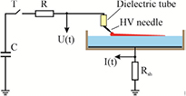
Figure 1. A general sketch of the experimental setup used for the study of transient streamers on the surface of tap water in air. C is a capacitor of 50 nF; R is a resistor of 1 kΩ; T is a thyratron; the HV needle is a sharpened wire 0.5 mm in diameter; the width and depth of the water basin are variable parameters; the length of the basin is 150 mm; the water basin is made of acrylic plastic.
Download figure:
Standard image High-resolution imageWe did not study the spatial-temporal behavior of the surface streamers using a fast frame camera with a short exposure time. The images of the SDL (top and side view) were taken by a CANON EOS-550D camera with a long exposure time; in fact, the obtained photos are the streamer images integrated over the whole life-time of the transient streamers. The required information about the dynamics of the streamers was obtained using light guides connected to photomultipliers and wire probes evenly distributed along the trajectory of the streamer (figure 2). The receiving ends of the light guides were placed over a streamer at a height of 4.5 mm, the wire probes were placed under the streamer in water with a depth of 1 mm. The electrical potentials on the HV needle and wire probes were measured by high-voltage probes (Tektronix P6015A). The electrical signals of the SDL current and voltage, as well as the signals of the wire probes and photomultipliers were recorded by a digital storage oscilloscope Tektronix TDS-520 (500 MHz, 1.0 GS s−1) and a Hewlett Packard oscilloscope (500 MHz, 1.0 GS s−1).
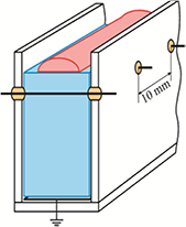
Figure 2. An illustrative sketch showing the cross-section of a narrow water basin with thin metallic wire probes for measuring the longitudinal electric field in the extending surface streamer (size proportions are not observed). The width of the water basin is 4 mm and its depth is 35 mm. The probes are made of wire 0.2 mm in diameter. The total number of probes is 12, and they are placed 10 mm apart and fully immersed in water with a depth of 1 mm.
Download figure:
Standard image High-resolution image3. Experimental results
Integrated images of the surface streamers propagating in shallow as well as deep open water, along with the inside wide and narrow dielectric channels are shown in figures 3–6. In these figures, the amplitude of the applied voltage U is a variable parameter.

Figure 3. Top view of the positive streamers on the open surface of the deep as well as shallow water. The photos are taken by a CANON EOS-550D camera with a long exposure time. For the denotation, U is the initial voltage of the charged capacitor C and h is the depth of the water in the basin. (a) h = 65 mm; U = 7 kV; (b) h = 5 mm; U = 7 kV; (c) h = 65 mm; U = 23.5 kV; (d) h = 5 mm; U = 23.5 kV.
Download figure:
Standard image High-resolution imageOne can see in figure 3 that, in general, the structure of the SDL on the surface of the open water looks as follows: there are several thick, bright primary streamers originating from the plasma region around the HV pin and extending more or less symmetrically in a radial direction. After reaching a critical length, several primary streamers undergo bifurcation, and each of the two arising streamer legs, in turn, can (but do not always) split again, and so on. The quantity of secondary streamers increases with a diminishing depth of water; the critical length for bifurcation diminishes with a decrease in the amplitude of applied voltage and the depth of water as well. After each bifurcation the light intensity of the arising secondary streamers diminishes; furthermore, the primary and secondary streamers are not smooth—they are surrounded with a 'thrum' of numerous thin, short and dim streamers directed at an acute angle to the body of the thick streamer. Finally, the described structure of the streamer is always surrounded by a diffuse glow plasma which homogeneously fills in all the space between the thin, short and dim streamers. So, the SDL makes contact with the water not only via the surface streamers but via the diffuse glow plasma as well. The total size of the area of water occupied by both the streamers and glow plasma increases with the amplitude of the applied voltage and the depth of the water.
In fact, the conductivity of the liquid leads to the surface streamer being shunted more strongly when the conductivity is higher. The heavy influence of water conductivity on the maximum length of the streamers propagating on the surface of open water is illustrated by the data in figure 4. The experiments were performed with a sectioned streamer discharge generated on the surface of both distilled water and tap water with a depth of 13 mm. The respective conductivities of the liquids are approximately 7.5 and 750 µS cm−1: i.e. the distilled water insulates rather more than the conductor. The HV sectioned electrode comprises five stainless needles linearly disposed 10 mm apart. A long grounded electrode with a width of 50 mm is placed on the bottom of the wide dielectric cell and is located to one side of the sectioned electrode. Such an electrode configuration allows us to confine the streamers within an area approximately 50 mm in width, which permits them to propagate in parallel. One can see in figure 4 that the streamers on the surface of the distilled water can be ignited by a lower voltage, and that they extend for a longer distance in comparison with those of the conductive tap water.
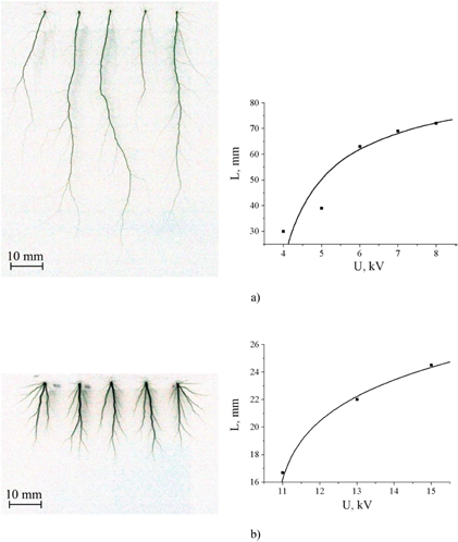
Figure 4. Negative images of the surface streamers in the sectioned SDL on the surface of the open water and the dependence of the maximum streamer length versus the amplitude of the applied voltage. The depth of the water is 13 mm. (a) Distilled water: the photo corresponds to the SDL powered by U = 8 kV; (b) tap water: the photo corresponds to the SDL powered by U = 15 kV.
Download figure:
Standard image High-resolution imageThe data presented in figures 5 and 6 demonstrates the structure of the surface streamers in the case when the space that is accessible to their propagation is restricted by the slit made in the dielectric plate placed on the water. Each long slit has a height of 4.5 mm.

Figure 5. A top view of the positive streamers on the surface of shallow water (h = 5 mm) restricted by long, straight dielectric channels. Every channel is a long slit made in the dielectric plate placed on the surface of the water; the channel height is 4.5 mm. The applied voltage and channel width are variable parameters. The length of the longest streamer is equal to 110 mm; such a streamer was obtained in a channel with a slit of 2.6 mm.
Download figure:
Standard image High-resolution image
Figure 6. A top view of the positive streamers in long dielectric channels placed on the surface of shallow as well as deep water. The slit width is 4 mm; the channel height is 4.5 mm; the amplitude of applied voltage is 23.5 kV.
Download figure:
Standard image High-resolution imageClose analysis of the data presented in figures 5 and 6 leads to several conclusions:
- (1)The decrease in the width of the slit results in the streamer branching diminishing and its length increasing.
- (2)The full absence of streamer branching and the maximum streamer length takes place in the slit with a width of less than 4 mm; in this case the streamers are smooth—they are not surrounded by the 'thrum' of numerous thin, short, dim streamers.
- (3)The maximum length for a non-branching streamer with a fixed slit width and water depth is reached in a deep, narrow basin like that in figure 2.
- (4)Both the brightness and diameter of the long streamer diminish in direction from tail to head.
- (5)Despite the restriction in the transverse direction, the straight-line trajectory of the long streamer is not stable—in fact, its form looks like a snake; the mechanism of the instability forming such a wavy trajectory is unknown.
- (6)An increase in the depth of the water results in an increase in the length of the streamer.
- (7)The higher the applied voltage, the longer the streamer.
The last statement is illustrated by figure 7, in which the dependence of the streamer length L versus the applied voltage U is shown. The data is presented for the SDL initiated in two narrow basins: (a) the width of the slit is 4 mm and depth of the water is 35 mm; (b) the width of the slit is 2.8 mm and the depth of the water increases from 35 mm at the tail of the streamer up to 100 mm at its head. As it turns out, in both cases the experimental data can be approximated by power functions with the powers close to 0.7: (a)  and (b)
  , with L in mm and U in kV. The magnitude U = 5.27 kV is equivalent to the threshold voltage for the ignition of the SDL under our experimental conditions.
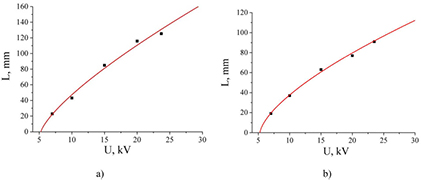
Figure 7. The dependence of maximum streamer length for the SDL in a narrow basin versus the initial magnitude of the applied voltage. The markers are the experimental data; the solid curves are the approximations by the power functions pointed out in the text. (a) The width of the slit is 4 mm and the depth of the water is 35 mm; (b) the width of the slit is 2.8 mm and the depth of the water increases exponentially from 35 mm at the tail of the streamer up to 150 mm at its head.
Download figure:
Standard image High-resolution imageThe resulting possibility of suppressing streamer branching and reaching a maximum streamer length at a fixed applied voltage is an attractive one from both the physical and practical point of view, because it offers great opportunities for significantly simplifying the mathematical modeling of the streamer on the surface of water and increasing the activation efficiency of the water by the SDL.
The next step in further improving the SDL system is the development of a sectioned SDL with long, isolated, non-branching streamers, each of which propagates inside its own narrow dielectric channel. We did this using a multichannel configuration comprising five parallel long, narrow slits in a dielectric plate placed on the surface of the water. The width of the slit was 3 mm, the thickness of the walls between the neighboring slits was 2 mm. Each of the five isolated streamers was initiated by an individual HV needle inserted into the slit. The obtained results in the form of images of the sectioned SDL (top view) are presented in figure 8. Examination of the images in figures 8(a) and (b) leads to the conclusion that the sectioned SDL with long streamers of practically the same length can only be created on the surface of shallow water. In the case of deep water there is competition between the strong streamers that results in the unequal redistribution of the electric current between them. This competition manifests itself in regular alternation of the long and short streamers in the neighboring slits. In the case of the sectioned SDL on the surface of open water (figures 8(c) and (d)), the competition between five short streamers for 'vital space' also exists and externally exhibits itself in the 'repulsion' of the streamers from each other, leading to their fan-shaped configuration. In total, the general trend for streamers on the surface of water can be formulated as follows: the maximum streamer length increases with the depth of the water in all configurations of the SDL.
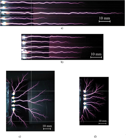
Figure 8. Images of the sectioned SDL initiated in the dielectric channels placed on the surface of water ((a) and (b)) and on the surface of open water ((c) and (d)). In all cases the amplitude of the applied voltage is 23.5 kV. (a) The depth of the water is 65 mm; the width of the slit is 2.5 mm; the length of the longest streamer is 115 mm. (b) The depth of the water is 5 mm; the width of the slit is 2.5 mm; the length of the longest streamer is 65 mm. (c) The depth of the water is 65 mm; the length of the longest streamer is 50–55 mm. (d) The depth of the water is 5 mm; the length of the longest streamer is 25–30 mm.
Download figure:
Standard image High-resolution image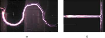
Figure 9. Control of the streamer configuration by the shape of the slit in a dielectric plate placed on the surface of the water. The depth of the water is 65 mm; the width of the slit is 2.5 mm; the applied voltage is 23.5 kV. (a) Sinusoidal configuration; (b) T-form configuration.
Download figure:
Standard image High-resolution imageAs shown above, the narrow, straight slit in the dielectric channel placed on the surface of the water strongly influences the streamers, resulting in the possibility of them extending over long distances. What about such influence in the case of slits with a non-straight configuration? We answered this question with experiments using dielectric plates with slits of a different non-straight configuration. As it turns out, it is quite possible to control the trajectory of the streamers and even forcibly to split them. Proper information is presented in figure 9. It is interesting to note that the double splitting (bifurcation) of the streamer in the channel of the T-form does not happen in the vicinity of the perpendicular wall, but a long way before it.
Another interesting question is as follows: is it possible for the surface streamer to penetrate through a thin dielectric film placed perpendicularly to its propagation? If yes, what is the mechanism for transfer of the current at this place: the displacement current through the solid film or the conductivity current through the film broken by the streamer? The answer to this question is not so evident. Indeed, it was shown in one paper [23] that a plasma jet can pass through a thin dielectric film due to the displacement current. However, in [14] it is shown that the streamer with the positive volume passes through a thin film of transformer oil only after breakdown of the film. To answer the question stated above we performed the experiment with a long isolated streamer initiated by a voltage of 23.5 kV. The streamer propagates in a narrow slit between two dielectric walls placed on the surface of the water. The thickness and height of the walls are 10 and 4.5 mm; the width of the slit formed by the walls is 2.8 mm. A thin film of mica with a thickness of 10 µm, a height of 10 mm and a dielectric permittivity ε = 6 was placed across the slit at a distance of 25 mm from the tip of the HV needle. The obtained visual information is presented in figure 10.
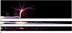
Figure 10. On the possibility of a streamer propagating through a thin mica film placed across a narrow slit. (a) The image (top view) of the SDL formed by the first voltage pulse: the streamer does not penetrate through the mica film due to the displacement current, but goes to one side and jumps over the thick dielectric wall to the water; (b) the image (top view) of the SDL formed by the second voltage pulse: the streamer eventually induces the electrical breakdown of the film followed by its perforation, penetrates through a small hole (30 µm) and propagates in a slit on the other side of the film; (c) the image (side view) of the SDL formed by the third voltage pulse: the streamer penetrates through a small hole created by the preceding SDL; the hole was created a little above the surface of the water due to the formation of a meniscus on both sides of the thin film.
Download figure:
Standard image High-resolution imageIt is well known that in DBD with a thick dielectric plate disposed in the middle of a short gap, fast microdischarges penetrate through the plate from one gas gap to another due to the displacement current. Analysis of the images presented in figure 10 leads to the conclusion that a long streamer slowly propagating on the surface of water cannot penetrate a thin dielectric film without it being perforated. In other words, the displacement current cannot provide the propagation of a slow surface streamer, even through a thin dielectric film with a high dielectric permittivity. In our experiments, the perforation of a thin mica film by the surface streamer does not happen at once, but only in the course of the second streamer stroke in the film.
The samples of the typical waveforms of the total electric current and voltage on HV needle of the pulsed SDL are shown in figure 11. The presented data corresponds to the SDL excited on the surface of shallow as well as deep water with and without the dielectric channel placed on it. In all cases, the capacitor C is charged up to a voltage of 23.5 kV. Note that the HV potential on the needle is equal to the total voltage drop across the whole SDL system, including the voltage drop along the streamer. The observed diminishing of the current and voltage after streamer breakdown is associated with the discharging of the capacitor C through the SDL system. Our measurements showed that the current decay lasts for almost hundreds of µs, or even longer. This means that the surface streamer on the water can also exist for such a long period. This feature of the SDL is attractive from both the physical and practical point of view, because it enables one to use a quasi-stationary approximation for modeling the late stage of the surface streamer and gives hope to being able to obtain a low-current steady-state SDL.
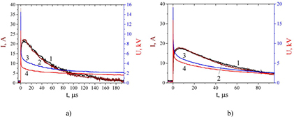
Figure 11. Typical waveforms of the total electric current (1, 2) and voltage (3, 4) on the HV needle of the SDL on the surface of shallow as well as deep water. (a) U = 23.5 kV, the depth of the water is 5 mm, (b) U = 23.5 kV, the depth of the water is 65 mm. Curves 1 and 3 correspond to the SDL in a slit 4 mm in width; curves 2 and 4 correspond to the SDL on the surface of the open water. At the same applied voltage, the maximum current through the liquid system is the same for the SDL in the slit and on the surface of the open water, although this current diminishes with an increase in the depth of the water in all cases.
Download figure:
Standard image High-resolution imageThe main conclusions derived from the data in figure 11 are as follows: (1) at the fixed water depth the total current through the SDL system is practically the same as for the SDL in the slit and on the surface of the open water; (2) the maximum current through the SDL system with the deep water is low compared to that with the shallow water; (3) the voltage drop across the SDL system with the shallow water is low compared to that with the deep water; (4) at the fixed water depth the voltage drop on the SDL in the slit is high compared to that for the case of the SDL on the surface of the open water.
The joule heating of the water by the electric current passing through the activated water is, in fact, a useless loss. The energy efficiency of the SDL in the activation of the liquid can be determined as the WS/WT ratio, where WS and WT are the instant electric powers deposited into the surface streamer and into the whole SDL system. Although most of the energy deposited into the streamer eventually goes towards the heating of the water, only the magnitude of WS determines the intensity of the biochemical activation of the water by the SDL. For general reasons one can say that the energy efficiency is high if the depth of the activated water is shallow, because the shallower the depth of the water, the smaller the voltage drop across it. However, of great practical interest is knowing the exact magnitude of the energy efficiency for a concrete SDL.
In our case, the values of WS and WT are determined in such a way: ![${{W}_{\text{S}}}(t)=I(t)\left[U(t)-{{U}_{12}}(t)\right]$](https://content.cld.iop.org/journals/0963-0252/26/2/025004/revision1/psstaa4bf9ieqn003.gif) ,
,  , where I(t) and U(t) are the instant total electric current and voltage applied to the SDL system, and U12(t) is the electric potential on probe # 12 located at the head of the streamer. We calculated the energy efficiency with the example of an SDL in a basin with a water depth of 35 mm and a slit width of 4 mm, powered by a voltage of 23.5 kV. Under these conditions the head of the long streamer reaches probe #12.
Proper information relating to the time behavior of the magnitudes of WS, WT and the WS/WT ratio in the pulsed SDL is presented in figure 12. The maximum instant electric power WT consumed by the SDL is high (up to 160 kW) and the total amount of energy deposited into the streamer is also high (up to several Joules). The energy efficiency WS/WT exhibits non-monotonic behavior in time, and maximum efficiency happens during the first 10 µs and after 150 µs of the SDL. An estimation of the reduced energy deposited into the body of the streamer gives a large amount of approximately several J cm−3; even more than that can increase the gas temperature in the streamer by up to several thousands of kelvin. This means that gas heating can play an appreciable role in both the mechanism of streamer propagation and the plasma chemistry in the streamer.

Figure 12. Experimental data (1, 2) on the time behavior of the electric power deposited into the streamer and the SDL and the calculated data (3) on the energy efficiency of the SDL. A transient discharge was initiated by the voltage with an amplitude of 23.5 kV in a basin with a water depth of 35 mm and a slit width of 4 mm. Curve 1: the total electric power WT(t), curve 2: the electric power deposited into streamer WS(t); curve 3: the energy efficiency of the SDL determined as the WS(t)/WT(t) ratio.
Download figure:
Standard image High-resolution imageThe primary information about the spatial-temporal dynamics of the long surface streamers was obtained from the measurements performed using photomultipliers (PMT) and wire probes disposed evenly along the streamer trajectory. The typical waveforms of the recorded PMT signals are presented in figure 13. This reveals the existence of two bright light waves attributed to the movement of the plasma regions possessing the higher electric field E/N. These waves are separated in time and move in opposite directions. The first wave (see figure 13(a)) is attributed to the movement of the bright head of the streamer at the stage of its extension from the HV needle. The velocity of the first wave is high at the HV needle and appreciably decelerates with an increase in the length of the streamer. The second wave (see figure 13(b)) is a slow one, is not so bright and happens later, when the current has lowered by at least twice the amount and the streamer strongly decelerates its extension until it has stopped completely. This wave reflects the decay of the streamer due to its cooling and moves in an opposite direction compared to the first wave, i.e. toward the HV needle. The characteristic time scales for the fast and slow waves differ by tens of times. The velocity of the slow backward wave is practically constant in time and equals 105 cm s−1.
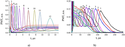
Figure 13. The sets of signals from the PMT relating to the fast direct (a) and the slow backward (b) light waves. The collecting light guides of the PMT are distributed evenly (1 cm from each other) along the trajectory of the streamer. The sensitivity of the PMT is the same for figures (a) and (b). The maximum streamer length is 125 mm. The transient SDL was initiated by a voltage with an amplitude of 23.5 kV in a basin with a length of 145 mm, a water depth of 35 mm and a slit width of 4 mm. The figure at each curve corresponds to the x coordinate (in cm) at which the collecting light guide was placed (x = 0 corresponds to the HV needle).
Download figure:
Standard image High-resolution imageThe spatial and temporal distributions of the fast wave velocity are derived from the PMT signals and shown in figure 14. One can see in figure 14(a) that the instant velocity of the streamer head appreciably diminishes with an increase in the streamer length. Nevertheless, the streamer extends up to practically 90% of its maximum length very quickly (in approximately 20 µs). After that, despite the diminishing discharge current, the streamer continues extending with a very low velocity until it reaches its maximum length. After a little while, the appearance of a slow backward wave is observed; this wave slowly travels towards the HV needle.
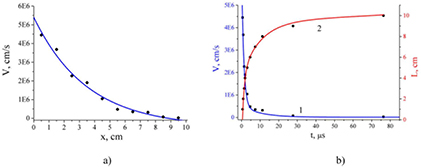
Figure 14. The parameters of the long streamer characterizing its propagation on the surface of water in a narrow channel 2.8 mm wide. The initial amplitude of the applied voltage is 23.5 kV. (a) The streamer velocity versus the instant streamer length; (b) the streamer velocity (curve 1) and the instant streamer length (curve 2) versus time. The markers are the experimental data, the solid curves are the smooth approximations of the experiment.
Download figure:
Standard image High-resolution imageThe data presented in figure 14 is complemented by table 1. This table contains information on the maximum length Lmax of the streamers at different applied voltages U and average streamer velocities  = xs/τ(xs) at different points xs of their trajectories, where xs is the distance of the chosen point from the HV electrode, and τ(xs) is the time spent by the streamer head in arriving from the HV electrode to point xs. The experimental conditions correspond to the SDL with tap water in a narrow channel 2.8 mm wide.
Table 1. The data on the maximum length Lmax of the streamers and the average velocities at different applied voltages.
| U, kV | 20 | 15 | 10 | 7 |
| Lmax, mm | 80 | 65 | 40 | 20 |
| xs, mm | 40 | 40 | 20 | 10 |
| τ(xs), µs | 4.1 | 10 | 18 | 34 |
 = xs/τ(xs), cm s−1 = xs/τ(xs), cm s−1 |
≈106 | 4 · 105 | 1.1 · 105 | 3 · 104 |
The electric field time dependence at different points along the streamer trajectory is shown in figure 15(a). The average electric field magnitude is derived from the probe measurements of the temporal dependence of the electrical potential Uk(t) on each wire immersed in water under the streamer:  , where l = 1 cm is the gap length between the two neighboring probes, k is the number of probes, and k = 0 corresponds to the HV electrode. The instant spatial profile of the electric field distribution (figure 15(b) corresponds to the classical distribution with a maximum field at the head and the low field in the body of the streamer. If the streamer length increases, the strength of the electrical field at the head diminishes. This fact correlates with the decrease in the velocity of the streamer when its length increases. At first glance, the electric field strength shown in figure 15 is low. However if we take into account a high gas temperature in the streamer, the reduced electric field E/N will be high enough to provide the necessary rate of ionization sustaining streamer propagation.

Figure 15. The spatial-temporal evolution of the electric field along the trajectory of the streamer in the course of its fast extension. The SDL is excited with an applied voltage of 23.5 kV in the water basin, shown in figure 2, with a slit width of 4 mm, a water depth of 35 mm, and a basin length of 145 mm; the maximum streamer length is 115 mm. (a) The average electric field versus time in different coordinates x of the streamer trajectory: curves 1, 2, 3, 4, 5, 6, 7, 8, 9, 10, 11 and 12 correspond to the coordinates x = 5, 15, 25, 35, 45, 55, 65, 75, 85, 95, 105 and 115 mm, respectively, measured from the HV needle; (b) the spatial distribution of the electric field along the streamer length at the moments corresponding to the maximums of curves 1–12 in figure (a): curves 1, 2, 3, 4, 5, 6, 7, 8, 9, 10, 11 and 12 correspond to t = 0.104, 0.216, 0.44, 0.74, 1.16, 1.724, 2.5, 3.528, 4.916, 7.0, 8.84, 11.216 µs, starting from the initiation of the SDL.
Download figure:
Standard image High-resolution imageWe simultaneously measured the x time dependence of both the electric field and light intensity in every coordinate for the fast direct and slow backward wave. The proper information is presented in figure 16 for the fast wave and in figure 17 for the slow wave. Curve 1 depicts the time behavior of the average electric field strength between the two chosen neighboring probes; curve 2 depicts the behavior of the light intensity in the x coordinates between the chosen probes. For presentation, the coordinates x = 5.5 cm and x = 9.5 cm have been chosen.
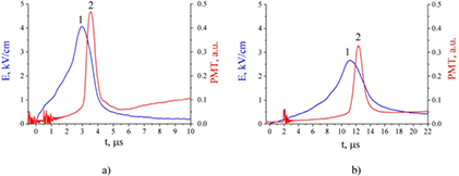
Figure 16. The time dependence of both the electric field and the light intensity at the same place for the direct fast wave. The experimental conditions correspond to those in figure 15. Curves 1 and 2 depict the time behavior of the electric field and the light intensity in the coordinate x = 5.5 cm (a) and x = 9.5 cm (b).
Download figure:
Standard image High-resolution image
Figure 17. The time dependence of both the electric field and the light intensity at the same place for the slow backward wave. The experimental conditions correspond to those in figure 15. Curves 1 and 2 depict the time behavior of the electric field and the light intensity in the coordinate x = 5.5 cm (a) and x = 9.5 cm (b). The peaks at t = 12 µs (a) and t = 24 µs (b) correspond to the direct wave.
Download figure:
Standard image High-resolution imageOne can see in figure 16 that the maximum electric field and the light intensity practically coincide in time at all the x coordinates (in fact, the maximum light appears a little later). In other words, the maximum light intensity in the direct fast wave is approximately located in the streamer head. In contrast, in the backward slow wave the maximum light intensity in every x coordinate appears much earlier compared to the maximum electric field strength (see figure 17). This effect is more pronounced for the parts of the streamer that are more distant from the HV electrode.
4. Numerical modeling and calculations
Adequate numerical modeling of the streamer propagation on the surface of water requires the use of a non-stationary 3D model, including a set of equations describing the charged and excited particle kinetics self-consistent with the Poisson and the gas heating equations. In such a formulation the task is too complicated for calculation, and beyond the scope of this paper. However, it is possible to simplify the task if there is no interest in the full dynamics of streamer propagation, but only in the spatial structure of the electric field E and the electric current I inside and outside the streamer. We offer a 3D steady-state approach which allows this to be done. The idea is based on the fact that the E, I spatial structure first depends on the geometry of the streamer and on the spatial distribution of its conductivity, and second is established much more quickly compared to the characteristic time for streamer propagation. In such a case, one can calculate the 3D E, I spatial structure inside and outside the streamer, if we suppose that the streamer parameters (conductivity, length, shape and transverse size) are preset and 'frozen'. This means that the 3D stationary model does not take into consideration the generation and recombination of the charged particles in the streamer, because their number densities are preset. The ionization of the air surrounding the streamer is also absent. So, the simulated non-branching streamer looks like a conductive solid body placed on the surface of the conductive water and surrounded by non-conductive air. The reasoning for using the simplified steady-state approach was taken from an experiment which showed that after fast extension the surface streamer slowly changes its length (see figure 14(b)), i.e. the streamer was practically motionless over a long time (at least 100 µs). This time is longer compared to the time determining the establishment of conductivity in the streamer.
This circumstance allowed us to use the static equations describing the E, I distribution. The steady-state approach means that the dielectric properties of the streamer–liquid system are inessential and the displacement current is out of consideration. The estimations for our experimental conditions proved that the contribution of the displacement current in the total current of the streamer–liquid system is negligible. To simplify the 3D calculations, we also assumed that the preset conductivity of the simulated streamer did not depend on either the time or the coordinate across and along the streamer. The characteristic streamer conductivity was chosenwto be about 1 S cm−1, corresponding to the electron number density of 3 · 1012 cm−3. Such an electron density is a typical value for many real streamers. The main goal of the simplified calculations is to obtain the general qualitative dependence of the E, I spatial structure on the preset streamer parameters. A variation of the streamer parameters within a reasonable range allows us to understand how the non-branching streamer chooses, for instance, the shape of its cross-section and the total transverse size.
The set of master equations of this model includes the equations of the electric current conservation in a liquid and plasma medium with their preset constant conductivities (σ = σp in the plasma and σ = σl in the liquid) and the Laplace equation for the electric potential in a gas medium (ambient air). The equations for both conductive media (plasma and liquid) are formally the same and are as follows:


where J is the electric current density, U is the electrical potential, σ is the electrical conductivity of the medium: σ = σp = 1 S cm−1 in the streamer and σ = σl ≈ 0.8 mS cm−1 in the liquid, i.e. σp  σl.
σl.
The boundary conditions for the potential U at the high-voltage electrode and the grounded electrode are U = UHV (preset) and U = 0 respectively. The UHV magnitude was varied within a range of 1–2 kV, corresponding to the SDL with long-living streamers. The normal components of the electric current at the streamer–gas, liquid–gas and liquid–dielectric wall boundaries are equal to zero. In other words, the electric current does not penetrate the gaseous or dielectric media from the streamer and liquid. Mathematically, this boundary condition is as follows:

where n is a vector normal to the surface.
It may appear that the space charge effects are totally neglected in this simplified model; in fact, this is not the case. The space charge effects are included in the model in the form of boundary conditions at the streamer–liquid, streamer–air and liquid–air interfaces. Indeed, the space charges are concentrated at the boundaries of the contacting media. In the case of a positive surface streamer there is a positive space charge in the thin layer adjoining the liquid; this layer is a cathode layer. The thickness of the glow cathode layer at atmospheric pressure does not exceed 5–10 µm, which is much less compared to the typical radius (1 mm) of the simulated streamer. The conductive positive streamer surrounded by the non-conductive air will also have a positive space charge at the streamer–air boundary. The thickness of this positive space charge is also very thin (⩽5–10 µm). The same situation exists for a negative space charge concentrated in liquid at the liquid–streamer and liquid–air boundaries. Due to the integration of the Poisson equation and using the Gauss theorem, the space charges concentrated in the thin layers at the boundary of two contacting conductive media can be attributed to the surface charges on the appropriate surfaces. In the case of our model, the local boundary conditions for the normal components of an electric field are as follows:
- (a)streamer–liquid boundary:
 ; ;
; ; - (b)streamer–air boundary:;
- (c)liquid–air boundary:.


Here Enp, Enl and Ena are the normal components of the electric field in the streamer, liquid and air; Sp and Sl are the positive and negative local surface charges on the streamer and liquid at the appropriate boundaries; σp and σl are the conductivities of the streamer and liquid.
The local boundary conditions for the tangential components of the electric field in all media are as follows:

The Laplace equation for the potential U in a gaseous non-conductive medium (air) is as follows:

The electric potentials in the gaseous domain at the streamer–gas and the liquid–gas boundaries are determined by the electric potentials at these boundaries formed by the electric currents in the liquid and plasma medium. In calculations, the configuration of the gaseous domain has a spherical form, and the electrical potential at its external boundary is equal to zero. In order to exclude the influence of the external boundary conditions on the results of the calculations, the chosen radius of the gaseous domain drastically exceeds all sizes of the rectangular dielectric basin.
A general isometric sketch of the configuration for the streamer–liquid system to be calculated is shown in figure 18. The chosen shape of the simulated surface streamer is a semi-cylinder with a spherically rounded head. The streamer is placed on the water and is located along the x coordinate symmetrically in the cross-section of the basin. The variable parameters were the depth h of the liquid and the diameter d and length l of the streamer.
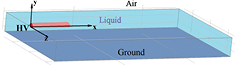
Figure 18. An isometric sketch of the configuration for the streamer–liquid system chosen for the calculation. The orientation of the unit vectors of the Cartesian system is shown.
Download figure:
Standard image High-resolution imageTo establish the semi-cylindrical shape of the simulated streamer, at the beginning we did a series of calculations of the E, I spatial structures around the streamer with its different shapes. Some of the results of these calculations are presented in figure 19. The upper row shows the set of the E spatial distribution around the streamer edge adjoining the water, and the bottom row shows the maps of the calculated I spatial distribution (current stream lines) for three different forms of the streamer cross-section. Note that all the streamers have the same envelope curvature radius (0.5 mm). The high magnitude of Emax obtained in the calculation is explained by the close proximity of the chosen cross-section to the HV electrode. The experiment shows that the effective radius of the real streamer at this place is larger than 0.5 mm.
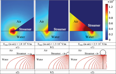
Figure 19. The enlarged simulated spatial structure of the electric field (upper pictures (a1), (b1) and (c1)) and the electric current stream lines (bottom pictures (a2), (b2) and (c2)) around the streamer on the water for different forms of its cross-section. The simulated streamer dimensions: the diameter of the envelope is 1 mm, the length is 5 mm, and the cross-section is taken at 0.25 mm from the HV electrode; this is a reason why the stream lines are strongly pressed to the bottom of the streamer. The dimensions of the calculated water domain are: width 15 mm, depth 2.5 mm, length 25 mm and U = 1 kV. (a1) and (a2) A flattened streamer with a cross-section which is only 10% of a circle with a diameter of 1 mm; (b1) and (b2) a semi-cylindrical streamer with a cross-section which is 50% of a circle with a diameter of 1 mm; (c1) and (c2) a protruding streamer with a cross-section which is 90% of a circle with a diameter of 1 mm.
Download figure:
Standard image High-resolution imageThe maximum electric field strength Emax in air happens at the streamer edge adjoining the water. In reality, ionization in the airspace with a strong electric field will lead to this space being filled with plasma. Due to this, the shape of the real streamer will deform until the magnitude Emax diminishes to Ecr, at which point the rate of electron ionization in the space will equal the rate of electron attachment. Figure 19 shows that the semi-cylindrical shape of the streamer cross-section provides the minimal magnitude of Emax among the three depicted forms of the streamer. So, we further used only the semi-cylindrical shape of the streamer cross-section with a diameter of 1 mm in the calculations. This diameter is typical for the real streamers observed in the experiments.
Figure 20 presents two maps of the calculated current streamlines in the SDL with shallow tap water and a surface streamer placed on the surface the open liquid. The left-hand picture is the map in plane YZ, x = 4.75 mm; the right-hand picture is the map in plane YX, z = 0. One can see that the area of liquid from which the streamer collects the electric current is large and appreciably exceeds the longitudinal and especially transverse streamer sizes. Because of this, the local current density in the lateral parts of the streamer contacting the liquid is slightly higher (about 20%) compared to that in the middle part of the streamer. Another feature is that the stream lines entering the streamer close to its tail are pressed more strongly to the bottom of the streamer compared to those entering close to the streamer head.
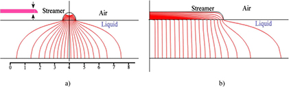
Figure 20. Two maps of the calculated current stream lines in the tap water system and the surface streamer placed on the surface of the open liquid. The diameter and length of the streamer are 1 and 5 mm respectively. The basin sizes: depth 2.5 mm, width 15 mm, and length 25 mm. The left-hand picture (a) is the map in plane (YZ, x = 4.75 mm); the right-hand picture (b) is the map in plane (YX, z = 0).
Download figure:
Standard image High-resolution imageIn contrast to the volume of the streamer propagating in a free space, the surface streamer collects the current not only through the head but also mainly through its lateral area adjoining the liquid. This is one reason why the average current density in the streamer cross-section increases with the distance from the streamer head. Figure 20(b) proves that the concentration of the current stream lines in the streamer body increases towards its tail. This can lead to the longitudinal component of the electric field in the streamer body also increasing towards the streamer tail.
The propagation of the streamer on the surface of the water is determined by the magnitude of the electric field in the air around it. One reason for this is that the ionization of the air adjoining the streamer generates plasma, forming a new part of the extending streamer. Figure 21 presents the pictures of the calculated distribution of the electric field modulus in three media—air, streamer and water—in an enlarged scale. The distributions are shown for the cross-section (YX, z = 0) in/around the short (5.5 mm) and the long (50.5 mm) simulated streamer. The long streamer is only partly shown (without its tail).
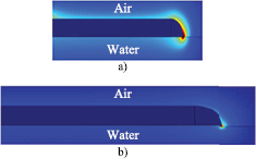
Figure 21. The simulated pictures for the spatial distribution of the modulus  of the electric field in/around the streamers on the surface of open water. The simulated streamers all have a diameter of 1 mm. Each picture shows the distribution in the plane YX, z = 0 (size proportions are not observed). The applied voltage is 2 kV; the depth of the water is 2.5 mm. (a) A short streamer with a length of 5.5 mm; the maximum
  in air is 2.45 · 107 V m−1; (b) the long streamer with a length of 50.5 mm; the maximum
  in air is 1.94 · 106 V m−1.
Download figure:
Standard image High-resolution imageDue to the high conductivity of the streamer compared to that for water and air, its electric field strength is lower than that in the water and air adjoining the streamer. As seen in figure 21, the maximum electric field Emax in air is concentrated around the head of the streamer. The calculations at a fixed applied voltage reveal that the Emax magnitude at the head of the streamer depends on its length: the longer the streamer, the lower the electric field. These simulated surface streamer features are illustrated in figures 21(a) and (b). Note that the calculated magnitude of Emax at the head of the short streamer exceeds the threshold magnitude Ecr =3 · 106 V m−1 corresponding to the streamer being stopped in air. This means that the simulated results can be attributed to the real streamer experiencing extension with a decelerating velocity.
Note that the results of the 3D numerical calculations point to a plausible reason for determining the diameter of the streamer. We have done the calculation for two simulated streamers on the surface of open shallow water (h = 2.5 mm) with diameters of 0.2 and 2.2 mm and a length of 80.5 mm. Figure 22 presents two simulated pictures depicting the E spatial distribution in air in the vicinity of the lateral parts of the streamer adjoining the liquid. For clarity, each picture only depicts a small piece of the body of the streamer and a small airspace surrounding the streamer, and an enlarged scale is used. Evidently, the strength of the electric field in the air around the thin streamer is higher than that around the thick streamer. Moreover, the strength of the electric field in air around the sidewall of the thin streamer twice exceeds the threshold magnitude Ecr at which ionization exceeds electron attachment. Such a high electric field promotes the extension of the thin streamer in a transverse direction up to a proper large size when the strength of the electric field at the sidewall diminishes at least to the threshold magnitude Ecr.
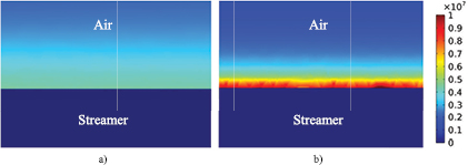
Figure 22. The pictures in the enlarged scale depicting the distribution of the modulus of the electric field in/around the simulated streamers on the surface of open water. The length of both streamers is 80.5 mm. The dark blue at the bottom is the streamer body part with a height of 50 µm. (a) The thick streamer with a diameter of 2.2 mm,  = 1.8 · 106 V m−1; (b) the thin streamer with a diameter of 0.2 mm,
  = 4 · 106 V m−1.
Download figure:
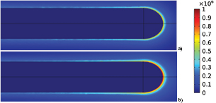
Standard image High-resolution imageThe experiment revealed that an appreciable restriction in the transverse direction of the area accessible to the propagation of the streamer on the surface of water leads to a strong increase in the length of the streamer. To gain an insight into the possible physical reason for this effect we performed 3D simulations for the long streamers on the surface of open water and in a narrow dielectric channel placed on it. The calculations were done using the example of deep water with a depth of 35 mm. The length and diameter of the simulated long streamer are 80.5 and 1 mm respectively; the slit width of the dielectric channel is 4 mm. The voltage applied to the simulated streamer–liquid system was taken to be the same as it is in the experiment. The obtained results under the same applied voltage are presented in figure 23. Each picture only depicts a small piece of the simulated streamer, including its forepart with the head, and an enlarged scale is used. A comparison of these pictures reveals that the E in air at the head of the streamer restricted by the narrow dielectric channel is appreciably higher compared to that for the streamer on the surface of open water. This calculated effect could explain why the real streamer extends over a longer distance in the narrow channel compared to the case of the open water. A comparison of the calculated maximum electric fields in air around the open ( = 8 · 105 V m−1) and restricted (
 = 4.16 · 106 V m−1) streamers with the threshold magnitude of Ecr = 3 · 106 V m−1 shows that the streamer that is 80.5 mm in length cannot be created on the surface of open water, correlating with the experiment.
Figure 23. The results of the 3D simulations for long streamers on the surface of open water (a) and in the narrow dielectric channel (b) (size proportions are not observed). The length and diameter of the streamer are 80.5 mm and l mm respectively; the depth of the water is 35 mm. The simulated streamers correspond to the second stage with a low applied voltage. (a) The streamer on the surface of the open water: the maximum electric field in the air at the head of the streamer is  = 8 · 105 V m−1; (b) the streamer in the narrow channel of 4 mm: the maximum electric field in the air at the head of the streamer is
  = 4.16 · 106 V m−1.
Download figure:
Standard image High-resolution image
5. Discussion
The subject of our discussion is the transient streamer discharges on liquid initiated by HV needles above it. At the very beginning, we have to emphasize the strong dissimilarity between these discharges with a different grounded electrode disposition. If the grounded electrode is disposed slightly above the liquid, the discharge channel always looks like a single, thick, bright current filament without any branching. As a rule, this filament slightly levitates above the liquid and the levitation is essentially of thermal origin. The detailed physical properties of such a discharge have been reported, for instance, in [24–26]. Note that this discharge has no similarity with SDBD.
Analysis of the experimental data showed that the spatial configuration of slowly developing and long lasting SDL on the surface of open tap water comprises, in the first approximation, the following basic structural plasma elements: the primary and secondary thick, bright, long streamers which are surrounded by numerous thin, dim, short streamers and diffusive glow plasma. The appreciable difference in the brightness of the thick and thin streamers and diffusive plasma is caused by the strong distinction in their conductivity which, in its turn, is determined by the magnitude of the electric current collected by each structural element. Every isolated thin streamer has a low conductivity (as well as glow plasma) and therefore collects a low current. However, all the thin streamers together provide a high current for every thick streamer. Due to this, high energy deposition into the thick streamers takes place, leading to their overheating and the development of ionization instability, resulting in a strong increase in streamer conductivity and an appreciable reduction in the strength of the electric field. The latter allows the extension of the thick streamer accompanied by the transfer of a high potential ahead where new structural plasma elements appear. In our opinion, the reason why the isolated primary streamer on the surface of open water cannot extend over a long distance is its bifurcation. In its turn, the bifurcation is initiated by one of the short, thin streamers, which, for some reason, has the necessary conditions for the development of the ionization instability that transforms the thin streamer into a thick, high conductive streamer joining the primary streamer.
Our findings, based on a statistical analysis of many SDL images on the surface of open water, showed that on average the thick primary streamer has a critical length beyond which bifurcation can happen. This length depends mainly on the applied voltage and water depth: the higher the applied voltage and water depth, the longer the critical length. Another finding is related to the properties of the short, thin streamers. As it turns out, there is a critical length for the free space around the thick streamer necessary for the development of short, thin streamers: they will not appear if the length of free space is shorter than the critical length. This means that there is a possibility of suppressing the development of these streamers geometrically. So, taking all this into account, one can conclude that the suppressing of short, thin streamers can remove the bifurcation of thick streamers as well. We did this by restricting the water area accessible for streamer expansion in the transverse direction. As a result, we were able to considerably increase the length of the isolated, thick, primary streamer and control the configuration of its trajectory. Most of our discussion is therefore devoted to the properties of the new object-long-lasting SDL with isolated non-branching primary streamers extending from the HV needle over a long distance.
Close examination of the obtained experimental data has revealed that the development of the SDL can be divided into two stages—a fast and a slow one—with a duration ratio between them of close to 1:10. The first stage correlates with the fast growth of the electric current accompanied by the quick extension of the streamer. Besides this, the extension of the streamer is accompanied by a wave of bright light emitted from its head. The second stage occurs with a slow diminishing current caused by a decrease in the voltage of the capacitor C feeding the SDL. Despite the diminishing discharge current, the streamer continues to elongate for some time, but with a decelerating velocity. Note that such streamer behavior in the SDL is similar to that in the SDBD observed in [27, 28]. More interesting is that the completion of the second slow stage corresponds to the streamer decaying, which is accompanied by the backward light wave. This wave has a lower light intensity and travels towards the HV needle with a constant velocity of about 105 cm s−1. The light emission of this wave is also attributed to the head of the streamer, meaning that the backward movement of the wave reflects the slow reduction of the streamer length. In other words, the surface streamer does not disappear simultaneously at once over all its length—it happens due to the slow diminishing of the length of the streamer.
The simultaneous dynamical measurements of both the electric field E(t) and the light intensity I(t) revealed a strong difference in the behavior of E(t) and I(t) for the direct and backward wave. To understand this difference, it is necessary to take into account that the intensity of light emission is determined by the local magnitude of the reduced electric field E/N, but not by the local electric field E. So, if there is a spatial inhomogeneity in the distribution of E and N, the maximum of E and E/N can appear in different locations. For the case of a fast, direct wave the maximums of the electric field and light intensity appear practically at the same time. Such a coincidence was observed for all the x coordinates. The mentioned good correlation in time of E(t) and I(t) is associated with two things: (1) the narrowness of the head of the streamer in the course of its extension, because it is only the signals from the head of the streamer that determine the behavior in time of the maximum electric field and light emission; (2) the low gas temperature gradient in the head leading to a spatial coincidence of the maximums of E and E/N. This low gas temperature gradient in the head of the streamer is explained by the fast propagation of the streamer through the non-preheated gas and the low energy deposition in the head. Note that the curves of the light signals I(t) around their maximums are narrower compared to those for E(t). A reason for this is the exponential dependence of the emission intensity on E/N in the case of the excitation of molecules by direct electron impact.
Another phase relationship between E(t) and I(t) was registered for the case of the backward wave: in every x coordinate the maximum light intensity appears earlier compared to the maximum electric field strength. This effect is more pronounced for the distant parts of the decaying and shortening streamer. The time difference for the appearance of the maximums of E(t) and I(t) in the backward wave can be explained by the fact that the head travels towards the HV needle through gas strongly and is non-uniformly preheated by the streamer at the preceding stage. A high gas temperature in the streamer body was observed, for instance, in [29–31].
We showed that the time dependence of energy efficiency of the slowly developing SDL is non-monotonic. We are not sure whether such a dependence is universal—this maybe an attribute of our specific method for the excitation of the SDL. However, the established properties of long streamers dependent on the depth and width of the basin for a single-pin and multi-pin electrode geometry have a greater generality.
The results on the spatial structure of E, I inside and around the simulated streamer obtained with 3D numerical modeling have helped us to develop an insight into the physics of real streamers.
First, the experiment in the sectioned SDL on the surface of open water and in parallel slits revealed the competition of the streamers, which manifests itself in their 'repulsion' of each other on the surface of the open water and in the regular alternation of long and short streamers in the neighboring slits. This competition can be understood if one takes into account the results of the calculations showing that the area of liquid from which the streamer collects the electric current is large and appreciably exceeds the longitudinal and especially transverse streamer sizes.
Second, the experiment showed that the streamer in the slit extends over a longer distance compared to that for the streamer on the surface of the open water. One of the reasons for this is pointed out by the calculations showing that the electric field strength in the air around the head of a restricted streamer is higher compared to that of a streamer of the same length on the surface of open water.
Third, the 3D calculations revealed that the increase in streamer length results in the diminishing of the strength of the electric field in the air around the head of the streamer—especially in its frontal part. This fact helps us to understand why the streamer slows down in the course of its extension.
Fourth, the calculations showed that the strength of the electric field in the air around the sidewall of the streamer with a smaller diameter is higher compared to that of the streamer with a larger diameter. This fact gives us an idea about how the restricted surface streamer establishes its diameter: the diameter of the streamer increases till the electric field strength at the sidewall diminishes to the threshold magnitude Ecr, when the rates of ionization and electron attachment equal each other. Note that the establishment of the transverse structure of the streamer on the surface of open water is a more complicated phenomenon because the body of the thick primary streamer is surrounded by thin streamers and glow plasma.
6. Conclusion
A pulsed slow-developing streamer discharge on the surface of water was investigated under conditions in which the displacement current plays a negligible role in the establishment of the discharge. The influence of the geometrical parameters of the water basin on the properties of the positive streamers was studied comprehensively. A new form of positive streamer extending over a long distance without branching was revealed. The properties of this streamer were explored thoroughly. Two stages in the evolution of long and non-branching streamers was revealed. The first stage is short and corresponds to the development of the streamer due to its fast extension. The second stage is relatively long and correlates to the disappearance of the streamer. It is important that the surface streamer does not disappear simultaneously at once over all its length; this happens due to the diminishing of the streamer length. As it turns out, the shortening of the streamer is accompanied by the formation of a backward light wave traveling towards the HV needle. This phenomenon was not described in the literature before, and has been discovered by us for the first time. The energy efficiency of the slow-developing streamer discharge with a long, non-branching streamer was estimated. The existence of non-branching long-living streamers not surrounded by either numerous, short, thin streamers or glow plasma enable us to simplify the modeling of the positive streamers. The 3D numerical calculations of the spatial structure of E, I inside and around the non-branching streamer were performed. The obtained results helped us to develop an insight into the physical properties of non-branching streamers.
We also found out that the streamer on the surface of conductive water differs strongly in comparison with both the volume streamer propagating through a gas gap and the surface streamer propagating on a dielectric barrier. The streamer on the surface of conductive liquid collects the conductive current from the liquid by the lateral surface adjoining it. However, both the volume streamer in the gas and the surface streamer on the dielectric collect the displacement current from the medium through/on which they extend: the volume streamer collects the current with its head from the space in front of it, and the surface streamer on the dielectric collects the displacement current with the lateral surface from the barrier. This is the main reason why the surface streamer on the conductive liquid can exist for a much longer time compared with both the volume streamer and the surface streamer on the dielectric, because these streamers require the displacement current for them to be supported.
Acknowledgments
The numerical part of this work was supported by the RSF (grant #16-12-10458), and the experimental part was supported by the RFBR (grants #15-02-06731, #16-02-00613) and COST Action TD1208.