
Abstract
The perpendicular propagation velocity of turbulent density fluctuations is an important parameter in fusion plasmas, since sheared plasma flows are crucial for reducing turbulence, and thus an essential input parameter for turbulent transport simulations. In the recent past various fusion devices have observed poloidal asymmetry in this velocity using Doppler reflectometry (DR) and correlation reflectometry. In this work, the phase screen model is used to analytically explain and quantify the combined effect of finite wavenumber resolution due to plasma curvature and probing beam geometry in a realistic turbulence wavenumber spectrum, leading to a reduced dominantly back-scattered wavenumber and a further underestimation of the perpendicular propagation velocity determined by DR. The full-wave code IPF-FD3D, which simulates microwave propagation and scattering, is used as a synthetic DR to study the effects of this diagnostic effect in a circular geometry using various isotropic synthetic turbulence wavenumber spectra. Angular scans from the midplane and variations in the position of the probing antenna are shown to estimate the impact of the diagnostic effect on the poloidal asymmetries.
Export citation and abstract BibTeX RIS

Original content from this work may be used under the terms of the Creative Commons Attribution 4.0 license. Any further distribution of this work must maintain attribution to the author(s) and the title of the work, journal citation and DOI.
1. Introduction
Turbulent energy and particle transport determine the energy confinement time of magnetically confined fusion plasmas [1]. Therefore, the study of turbulence and its underlying mechanisms is of particular importance for the prediction of fusion reactor performances.
Turbulence in a system is characterized by its wavenumber power spectrum  , which indicates the distribution of energy over the different scales of turbulence that are defined by their wavenumber k [2]. Due to the strong background magnetic field in fusion plasmas, the observed turbulence is approximately two-dimensional (2D) in the plane perpendicular to the magnetic field lines,
  [3]. The particular scales, where an instability injects energy into the system is known as injection region, often referred to as the knee position
  . The energy is further transferred to other scales, forming a cascade
  , defined by the spectral index α [4]. In 2D turbulence, two cascades emanate from the injection region. An inverse energy cascade towards larger scales and a direct enstrophy cascade towards smaller scales [5, 6].
Moreover, strongly sheared flows can tilt and decorrelate the turbulent structures. Hence, this mechanism suppresses the turbulence, forms a transport barrier [7], and thus gives a possible explanation for the occurrence of the high confinement mode (H-mode) [8].
Experimentally, the turbulence wavenumber spectrum and the turbulent structure's velocity in the plasma confined region can be measured by several reflectometry techniques. This paper focuses on Doppler reflectometry (DR) [9] that measures the turbulent scale dependent back-scattered microwave power  . From the frequency spectrum, the turbulent power
  and perpendicular propagation velocity
  of turbulent density fluctuations can be inferred, where
  is the E × B-drift velocity and
  is the intrinsic phase velocity of the density fluctuations. Here, the term perpendicular refers to the binormal direction to the magnetic field and the flux surface normal. The phase velocity is usually small compared to the E × B-velocity,
  [10, 11] (and references therein), such that the variation of
  is mainly driven by the poloidal variation of the background magnetic field and the radial electric field Er
, that varies due to flux compression via the Grad–Shafranov shift.
is mainly driven by the poloidal variation of the background magnetic field and the radial electric field Er
, that varies due to flux compression via the Grad–Shafranov shift.
Recently, the TEXTOR tokamak [12], the Tore Supra tokamak [13], and the TJ-II heliac [14] have reported on poloidal asymmetries in the perpendicular propagation velocity of density fluctuations, that are beyond the poloidal variation of the E × B-drift velocity. Subsequent experiments on ASDEX Upgrade (AUG) [11] showed no poloidal asymmetries. Detailed attempts to explain the observed asymmetries with respect to the underlying physics are presented by [13, 14], however none of those completely explain the phenomenon and the asymmetries' origin is still under investigation.
Due to the high complexity of the DR diagnostic, the measurements can be subject to systematic diagnostic effects, e.g. toroidal mismatch angle attenuation [15, 16]. Previous studies addressing the diagnostic impacts on the perpendicular velocity measurements with 2D full-wave analysis are shown in the references [17–19]. They investigated the effects of increased turbulence levels, spectral resolution, and tilt angle. Their work shows that even relatively large fluctuation amplitudes do not significantly affect the perpendicular velocity measurements. However, they discuss a diagnostic effect that leads to an underestimation of the perpendicular velocity, henceforth referred to as  -underestimation effect. The effect results from the finite beam width and, thereby, spectral resolution at the cut-off. Thus, not only the desired
  but a range of wavenumbers in the wavenumber spectrum of the turbulence is probed. In a realistic decaying turbulence wavenumber spectrum, this always leads to a smaller, dominantly back-scattered wavenumber and thus to a systematic underestimation of the perpendicular velocity, which, as shown in this paper, should also be considered as a contribution to the poloidal asymmetries.
Section 2 introduces the diagnostic technique and its limits in spectral resolution. Extending the previous studies of the  -underestimation effect, section 3 presents an analytic estimate of the velocity deviation. The analytical analysis is accompanied by 2D full-wave simulations using the finite-difference time-domain (FDTD) full-wave code IPF-FD3D [20] presented in section 4, where the effect's impact on the poloidal asymmetries is investigated in a circular geometry by performing poloidal scans in injection angles and variation of the launching antenna. Last, in section 5, the results are summarised and discussed.
2. Doppler reflectometry
DR (or Doppler back-scattering (DBS)) [9, 21] is a microwave diagnostic technique that measures spatial and wavenumber resolved turbulent density fluctuation powers  and their perpendicular propagation velocities
  . Microwave beams of ordinary (O-mode) or extraordinary (X-mode) wave polarization are launched into the plasma using an oblique injection angle θ with respect to the flux surface normal. Passing through denser plasma, the wave is refracted and eventually reflected at the cut-off layer, where the refractive index N is minimal. Parts of the wave are scattered by turbulent density structures at the cut-off layer. Using a monostatic antenna configuration, the back-scattered signal corresponds to the perpendicular wavenumber
  , which satisfies the Bragg condition of order
  . k0 is the vacuum wavenumber
  , with launching frequency f0 and vacuum speed of light c. To determine the refractive index
  at the cut-off, ray or beam tracing techniques are usually applied.
Due to a perpendicular velocity, the back-scattered signal becomes Doppler shifted by fD , such that
In experiments, this perpendicular velocity  is the velocity of the fluctuations in the laboratory frame, where
  is the E × B-drift velocity and
  is the intrinsic phase velocity of the density fluctuations.
DR commonly uses heterodyne signal detection [22], providing a complex IQ-signal. The back-scattered power  and the Doppler frequency fD
are determined from the power spectral density. By sampling several perpendicular wavenumbers through a tilt angle scan, a power spectrum is obtained. The same analysis tools are used in the following to analyze the IPF-FD3D simulation outputs.
and the Doppler frequency fD
are determined from the power spectral density. By sampling several perpendicular wavenumbers through a tilt angle scan, a power spectrum is obtained. The same analysis tools are used in the following to analyze the IPF-FD3D simulation outputs.
For small density fluctuation levels  , with nc
being the background electron density at the wave's cut-off and
, with nc
being the background electron density at the wave's cut-off and  the root mean squared of the density fluctuations, the linear scattering theory holds. Then, the power scales as
  , where
  is the underlying normalized perpendicular wavenumber spectrum of the density turbulence [9, 23, 24]. This linear approach is typically only valid in the plasma core. For higher fluctuation levels non-linear scattering may lead to an enhanced or saturated power response [25, 26].
The measurement's accuracy is limited by the spectral resolution  of the DR [27]. Accordingly, DR probes several wavenumbers in a range of
  , where
  is the central probed wavenumber. In the linear scattering theory, the back-scattered wave electric field
  can be found applying the reciprocity theorem [23, 24] or the physical optics model [26], such that in the k-space

where  is the probing beam's electric field, that acts as a filter in k-space.
Assuming the microwave beam to be a Gaussian defined by its beam width w, vacuum wavenumber k0, and beam curvature radius Rb
, the spectral resolution including curvature effects can be estimated analytically using a phase screen model
7
[9, 28]. Defining the beam's electric field according to the IPF-FD3D code as  the
the  -width of the beam's power at the cut-off is given by
with the effective radius  , where Rc
is the plasma curvature radius.
, where Rc
is the plasma curvature radius.  is the effective beam waist, which includes the effect of geometric projection of the beam in the direction of the reflecting layer caused by the oblique incidence with the angle θ. In this work, Rb
and w are approximated by Gaussian beam propagation in vacuum starting from the beam waist w0 [9, 29], which is intrinsic to the antenna of the DR system. Since the propagation characteristics may differ significantly from those in vacuum [15], for further analysis of the
is the effective beam waist, which includes the effect of geometric projection of the beam in the direction of the reflecting layer caused by the oblique incidence with the angle θ. In this work, Rb
and w are approximated by Gaussian beam propagation in vacuum starting from the beam waist w0 [9, 29], which is intrinsic to the antenna of the DR system. Since the propagation characteristics may differ significantly from those in vacuum [15], for further analysis of the  -underestimation effect, a more sophisticated beam tracing code should be used. Alternatively, the spectral resolution can be determined directly by the analysis of the weighting function using full-wave simulations [30]. A comparison between the different methods is given in Conway et al [29]. The analytical approximation in (3) therefore slightly overestimates the spectral resolution with respect to the weighting function approach, it is however sufficient to understand the observed trend in the velocity measurement, as shown in section 4. While for slab geometry (
 ), the spectral resolution can be increased further by increasing the beam waist w0, it is limited in real fusion experiments where the plasma curvature and thereby
  are finite. Then, an optimal beam waist
  exists, for which
  is minimal. At AUG typically a spectral resolution of
  can be reached [31]. For future DR systems at ITER a slightly increased spectral resolution of
  is to be expected [32].
3. Analytic analysis of the
 -underestimation effect

Since the probing beam  scans a certain wavenumbers range that is defined by the beam's spectral resolution
  , it filters the spectrum according to equation (2). The turbulence scales will contribute to different extent according to the realistic turbulence power laws. As shown in figure 1, the main back-scattered wavenumber
  is therefore different from the thought probed wavenumber
  . If unaware, this leads to a systematic
  underestimation in the measurements. To estimate the
  -underestimation effect analytically, the convolution in (2) is evaluated. The Gaussian electric field distribution of the probing beam is described by

where  is the central probed perpendicular wavenumber and
  the spectral resolution from (3). To study the effect of the turbulence wavenumber spectrum, a continuously decaying spectrum

is assumed. Thus, equation (5) describes piece-wise realistic turbulence wavenumber spectra as elaborated in section 1. Remark here, that  , since α is the spectral index of the power spectrum
  . Evaluating the convolution (2), the wavenumber with the highest back-scattering intensity
  can be retrieved from
  . A ratio X between the dominantly back-scattered and originally aimed wavenumber can be obtained
where the impacts of the finite spectral resolution and the turbulence wavenumber spectrum are manifested in  and η, respectively. Equation (6) shows that, since a finite spectral resolution is experimentally unavoidable, a spectral decay in the turbulence spectrum always manifests itself in a smaller dominantly back-scattered wavenumber. A maximum of the convolution
  and further a real solution for (6) only exists if
A maximum underestimation of 50% is obtained when  . Then,
  corresponds to a saddle point. When (7) is not fulfilled, the spectral decay dominates since
  and no maximal back-scattered wavenumber can be determined. Nevertheless, as shown by the full-wave results in section 4, the deviation can even exceed 50% for realistic turbulence spectra.

Figure 1. Example wavenumber spectrum for 2D turbulence. The back-scattered beam (red) is the result of the probing beam (blue) and the wavenumber spectrum (black). Due to the spectrum's decay and the finite spectral resolution, the maximum of the back-scattered beam  is reduced with respect to probed beam maximum
  .
.
Download figure:
Standard image High-resolution imageThe described effect further affects the determination of the perpendicular velocity since the central probed wavenumber  is used in (1). If the underlying turbulence spectrum is known, the ratio X can be used to predict the measured perpendicular velocity

The measured velocity is thereby always lower than the actual velocity.
Figure 2 shows the ratio  as a contour plot. The contour line of X = 0.9 is shown explicitly and marks the parameter range up to which the
  -underestimation effect is still below 10%. The white area in figure 2 marks the parameter range for which, according to condition (7), no main back-scattered wavenumber
  can be found. The contour plot emphasizes that there is no deviation for flat spectra (
 ) or for perfect spectral resolution (
 = 0 cm−1). The more the spectrum decays or the broader the spectral resolution, the stronger the deviation.
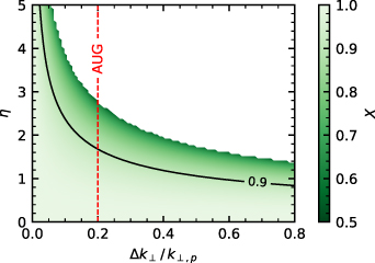
Figure 2. Contour plot of ratio X in (6) in dependence on the spectral decay index η and the spectral resolution  . The contour X = 0.9, up to which the deviation is below 10%, is shown explicitly. The approximate spectral resolutions of AUG is indicated as red dashed line. No solutions for X can be found in the white area.
Download figure:
Standard image High-resolution imageWhile the spectral decay η is a property of the plasma turbulence, the spectral resolution is inherent to the DBS system and the cutoff layer curvature. As explained in section 2, it can be optimized but is limited for curved geometries. The spectral resolution of the AUG steerable system [31] in figure 2 illustrates that even for a DR system with an optimized resolution, the deviation can become decisive for strongly decaying turbulence wavenumber spectra.
Besides the effect's contribution to poloidal asymmetries, it also becomes relevant in the determination of the turbulent phase velocity  , that is typically less than 2 km s−1 [31, 33], and relies on the accuracy of the DR measurements.
4. Full-wave simulations with IPF-FD3D
4.1. IPF-FD3D simulation setup
The DR simulations are performed with the FDTD code IPF-FD3D [20]. The code simulates microwave propagation in plasmas by solving Maxwell's equations in the cold plasma approximation with the plasma response calculated from the electron equation of motion. The partial differential equations are implemented as finite difference equations on a spatial Cartesian Yee grid [34]. A temporal leapfrog scheme is applied. The electron response is integrated separately using a modified Crank–Nicolson method [35]. The system of equations can be solved in two and three dimensions. The presented simulations use the 2D version of the code, so they do not include 3D effects and  .
.
Input to the simulation are spatial arrays of the background electron density  and the magnetic field
  . In the presented investigations, these are based on the AUG midplane profiles measured in AUG discharge #31 260, shown in figure 3. The poloidal magnetic field was set to zero in this study. A circular geometry is used, that is centered at
  m and has a curvature radius of
  0.4 m for a cut-off at
  . The geometry is poloidally symmetric and there is no Grad-Shafranov shift. Figure 4 shows the poloidal cross-section of the corresponding magnetic flux surfaces and X-mode cut-off frequency
  contours. The O-mode cut-off contours are not shown since they are aligned with the magnetic flux surfaces.

Figure 3. (a) Electron density profile and (b) toroidal magnetic field profile for the full-wave simulation. The poloidal magnetic field was set to zero in this study. Both profiles are from AUG discharge #31 260.
Download figure:
Standard image High-resolution image
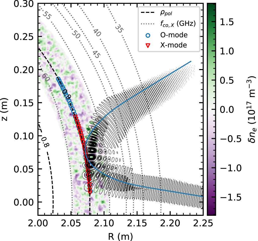
Figure 4. Section of the circular plasma cross-section with poloidal flux surfaces (dashed, black) and X-mode cut-off frequency contours (dotted, gray) and overlaid synthetic density fluctuations. The full-wave measurement locations using a midplane antenna at (2.3,0.0) m are indicated for O-mode (blue, circles) and X-mode (red, triangles). A sample beam trajectory obtained from ray-tracing calculations is shown in solid blue. The corresponding electric field from the full-wave simulation is shown by the black contours, where stronger contours correspond to stronger electric field.
Download figure:
Standard image High-resolution imageThe circular geometry allows the modeling of bulk plasma flow using synthetic turbulence, where the input-output comparison as well as the identification of diagnostic effects becomes straightforward. The modeling of turbulence in more realistic geometries, such as the ordinary D-shape, would require sophisticated plasma turbulence simulation codes such as GENE [36].
The isotropic synthetic turbulence pattern used in the presented simulations is based on an initial set 2D turbulence spectrum model  that has the Kolmogorov-like form
where  and
and  cm−1 is the chosen transitional wavenumber. Remark that the retrieved power spectral index is
  . From
  , the turbulence pattern is created using a 2D inverse fast Fourier transform as shown in Pinzón et al [26]. It is normalized to the intended turbulence level and applied as a band at the flux surface of interest, here
  as shown in figure 4. Due to the fast time scales of microwave propagation, the turbulence can be assumed to be frozen. Thus, the perpendicular plasma motion is modeled by rotating the turbulence band by an angle θrot
each time step
as shown in figure 4. Due to the fast time scales of microwave propagation, the turbulence can be assumed to be frozen. Thus, the perpendicular plasma motion is modeled by rotating the turbulence band by an angle θrot
each time step  . For a constant rotation velocity
  the time resolution is therefore determined via
  , where
  and
and  the radial turning point (t.p.) position with respect to the plasma center, that is determined using ray tracing. The turbulence is thereby rotating as a bulk without a wavenumber-dependent phase velocity. A full-wave simulation is performed in each turbulence frame, resulting in a time-dependent output, which can be analyzed in the same manner as discussed in section 2. Since the turbulence is frozen, the simulation is entirely independent of the velocity and only used for the signal analysis via
  . It is normalized to the intended turbulence level and applied as a band at the flux surface of interest, here
  as shown in figure 4.
The following subsections present full-wave results of two different synthetic turbulence patterns. Both spectra  are Kolmogorov-like as (9) and have a knee position at
  cm−1. A flat-top decay spectrum that is flat up to the knee position,
  , and then decays with a spectral index of
  as well as a more realistic 2D-Kolmogorov spectrum with two spectral decays
  and
and  . The latter corresponds to a turbulence wavenumber spectrum observed in 2D neutral fluids [5]. A low turbulence level of
  0.1% is used for all the presented simulations to ensure a linear power response. An input velocity of
  km s−1 is chosen, which is of an order of magnitude that is typically measured in fusion experiments.
The microwave beam model is a fundamental Gaussian, specified by its input frequency f0 and beam waist w0 at the antenna location, where the beam curvature is zero. The irradiation angle θ is defined with respect to the R-axis. In contrast to the experiment, where the beam waist w0 usually scales with  [37], it is kept constant at
  mm for all simulations. A similar frequency-dependent adaptation of w0 could be illuminating in future work.
The simulation launches several frequencies simultaneously. For signal discrimination, all the applied frequencies must be different by integer multiples of a constant frequency step typical of the order 100 MHz. Sufficiently refined time stepping is ensured by choosing a reference frequency larger than any probing frequency that determines the simulation time step  . An exemplary electric field pattern obtained from the full-wave simulation is shown in black contours in figure 4.
4.2. Effect of the turbulence wavenumber spectrum
As elaborated in section 3, the magnitude of the  -underestimation effect depends on the decay of the turbulence wavenumber spectrum
  and the spectral resolution
  . According to figure 2, the steepness of the turbulence wavenumber spectrum η determines thereby the extent to which the back-scattered wavenumber
  and thus the perpendicular velocity will deviate from the central probed wavenumber
  , and the actual velocity, respectively.
Figure 4 shows the simulation setup, with the antenna located on the midplane. Frequencies f0 and injection angles θ are defined to have their cut-off at  using a ray tracing code. Thereby, the velocity is measured at different poloidal locations for
  = 2–20 cm−1. Thus, frequencies fO
= 58–77 GHz for O-mode and fX
= 92–98 GHz for X-mode and injection angles in a range of θ = 2–24∘ are used. The corresponding spectral resolutions
= 2–20 cm−1. Thus, frequencies fO
= 58–77 GHz for O-mode and fX
= 92–98 GHz for X-mode and injection angles in a range of θ = 2–24∘ are used. The corresponding spectral resolutions  that are obtained using (3) are shown in figure 5. They differ by polarization due to the different frequencies applied to achieve the same cut-off.

Figure 5. Spectral resolution  computed using (3) for O-mode (blue) and X-mode (red) for the full-wave simulations with the antenna located on the midplane. Corresponding turning points are shown in figure 4.
Download figure:
Standard image High-resolution imageThe full-wave results of the turbulence wavenumber spectra are shown in figures 6(a) and (b). The enhanced decays in the back-scattered powers  obtained by the analysis of the complex IQ-signal are related to the scattering efficiency and are corrected using
 ![${P_{\mathrm{corr }}(k_{\perp}) = P(k_{\perp})\left[1+\left((L^{\mathrm{ref}})/(8 k_{0}^{2})\right)^{2 / 3} k_{\perp}^{2}\right]}$](https://content.cld.iop.org/journals/0741-3335/65/6/065010/revision2/ppcfaccd1aieqn117.gif) , where
, where  is the refractive index scale length [26]. The corrected spectra show excellent agreement with the spectral decay in the input spectra for both turbulence patterns and polarizations and are thus a good reference for the velocity studies.
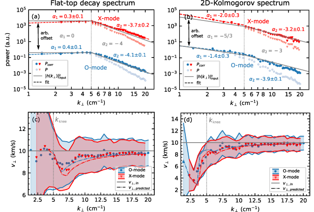
Figure 6. Full-wave simulation results for O-mode (blue, circles) and X-mode (red, triangles) for a flat-top decay spectrum in (a) and (c) and a 2D-Kolmogorov spectrum in (b) and (d). The input spectra and input perpendicular velocities are shown in solid gray. The turbulence wavenumber spectra results are shown in (a) and (b). The full symbols represent the corrected results regarding the scattering efficiency. Fits for the spectral indices α are shown in dashed lines. The perpendicular velocities are shown in (c) and (d). The shaded area marks the uncertainty band, that result from the spectral resolution  and the fit error on the Doppler shift frequency
  , and the numerically predicted velocities via (8) are shown dash-dotted.
Download figure:
Standard image High-resolution imageAs to be expected from the previous discussion on the  -underestimation effect in section 3, the full-wave results of
  in figures 6(c) and (d) are mainly below the input velocity. Both spectra exhibit a drop in the measured velocity around the knee position
  . The flat-top decay spectrum's drop recovers for
  before it exceeds 20% deviation since η and therefore X becomes zero. In contrast, the velocity in the 2D-Kolmogorov spectrum reduced up to 70%. For the same reasons as for the flat-top decay spectrum the velocities start to recover for
  cm−1, when they approach the transitional wavenumber
  . Due to the decreasing spectral resolution
  towards higher wavenumbers (see figure 5), the velocities approach the actual velocity accordingly.
Since the studied turbulence spectra are not differentiable at  and
and  a numerical determination of the convolution in (2) is necessary to predict the velocity deviation, according to (8). The same also applies to analyses carried out with discrete simulation outputs. Figures 6(c) and (d) show these numerical results of
  for the two synthetic turbulence spectra and polarizations, respectively. They were obtained using the input turbulence spectra shown in figures 6(a) and (b) and the spectral resolutions shown in figure 5.
We can observe that O-mode and X-mode predictions show excellent agreement with the full-wave results' trends, indicating their attribution to the  -underestimation effect. Similarly, good predictions of the
  -underestimation effect are obtained for a flat and Gaussian spectrum for slab and circular geometry. The interested reader is referred to Frank [38]. However, the predicted velocities exhibit slightly more deviation in X-mode than in O-mode due to the increased
  as shown in figure 5. Similar difference between X- and O-mode full-wave results is not in evidence.
Remark that the  -underestimation in the 2D-Kolmogorov spectrum in figure 6(d) reaches a parameter space in the ratio X that is not reachable in the analytical treatment presented in section 3. Both numerical results show that real solutions exist even if (7) is not satisfied. Since, contrary to the initial assumption in (5), the turbulence spectra for
  do not diverge but flatten (see (9)), the deviation can even exceed a factor of 2.
The differences of magnitudes in the deviations in the full-wave results and the results obtained by numerical convolution highlight the sensitivity of the  -underestimation effect to the underlying turbulence wavenumber spectrum. Especially for lower wavenumbers, where the relative spectral resolution
  can be poor, the deviation becomes large for realistic turbulence spectra. The angular scan, and thereby scan in poloidal direction, revealed that strong spectral decays in the turbulence spectrum and non-optimized spectral resolution of the DR lead to apparent poloidal asymmetries due to the
  -underestimation effect.
4.3. Poloidal variation of the antenna position for X-mode
The full-wave simulation's flexibility allows studying the influence of the poloidal probing position on the  measurement with DR. Moving the antenna towards the top, the
  -underestimation effect is affected by the background magnetic field leading to modified X-mode cut-off layers with respect to the poloidal flux surfaces, as shown in figure 7.
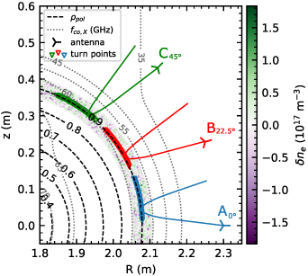
Figure 7. Antenna positions and measurement positions to study the poloidal variation of the antenna position using X-mode probing in the circular geometry introduced in section 4.3. All antennas are in the same distance from the plasma center. Poloidal flux surfaces are shown in dashed black and X-mode cut-off frequency contours in dotted gray. The turbulent density fluctuations are overlaid.
Download figure:
Standard image High-resolution imageInvestigations on O-mode are not shown, as its propagation depends only on the background electron density, which is poloidally symmetric in the present geometry. The interested reader is referred to Frank [38].
Figure 7 shows the three antenna positions and corresponding turning points, which probe the plasma with the same distance to the flux surface of interest and correspond to poloidal angles of 0∘, 22.5∘ and 45∘ with respect to the midplane. Basis of all three simulations is the flat-top decay spectrum shown in figure 6(a). The magnetic field dependence manifests itself in the X-mode dispersion relation, such that the frequencies used in order to reach  are increased the more upwards the antenna is moved,
  GHz,
GHz,  GHz,
GHz,  GHz.
GHz.
The increased input frequencies lead to increased spectral resolutions  in (3) and thereby increase the
  -underestimation effect. This is reflected in the predicted velocities
  in figure 8. They show a slightly increased deviation when changing the antenna location, as further indicated by the drop minimum in the figure. While similar trends are observed in the full-wave results, they show more spread between the antenna locations than the predictend curves. Direct effects on the beam width due to cut-off variation via the background magnetic field are not considered in the estimation of the spectral resolution and the diagnostic effect in (8) via the phase screen model, assuming vacuum propagation. Thus further elaboration to reproduce the enhanced spread in the predicted velocities requires more sophisticated beam models or full-wave simulations to estimate the spectral resolution in X. However, the small difference between full-wave and predicted velocity results highlights the robustness of the herein-applied method to assess the
  underestimation.
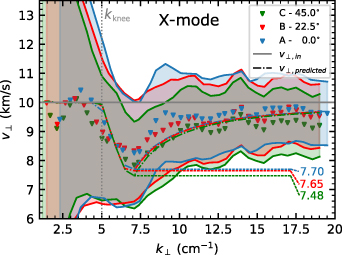
Figure 8. Perpendicular velocities from full-wave simulations for the three antenna positions and corresponding turning points in figure 7. The input velocity is shown in solid gray. The shaded area marks the uncertainty band and the numerically predicted velocities via (8) are shown dash-dotted.
Download figure:
Standard image High-resolution imageOverall both predicted velocities and full-wave results indicate that the poloidal asymmetry caused by the  -underestimation effect and change in the poloidal position of the antenna is only marginal. Significant deviations due to a variation in the antenna position are thus not expected in the experiment.
5. Summary and discussion
DR simulations were carried out to study poloidal asymmetries in the perpendicular velocity measurement, which have been observed on several devices in the recent past.
The  -underestimation effect was quantified analytically. An expression was derived in (6) describing the deviation in the perpendicular velocity when the underlying turbulence wavenumber spectrum exhibits a continuous spectral decay. The full-wave simulation code IPF-FD3D was used on synthetic isotropic turbulence in a circular plasma geometry to simulate the wave propagation and its scattering with constant turbulence rotation. The asymmetries were investigated concerning the influence of the underlying turbulence wavenumber spectrum and the background magnetic field due to the variation of the poloidal antenna position.
The  -underestimation effect was estimated numerically for two exemplary turbulence wavenumber spectra, showing excellent agreement with the full-wave results' trends. The investigations showed that an effect of 10% is very likely in actual DR experiments. However, performing measurements under poor conditions, e.g. in the low k range or on strongly decaying turbulence spectra, can lead to a velocity underestimation of even more than 50%.
The  -underestimation effect leads furthermore to apparent poloidal asymmetries when wavenumbers of different ranges and, therefore, different spectral decays of turbulence are probed in poloidally separated regions. However, the experiments at TJ-II [14] revealed that poloidal asymmetries also appear when the probed wavenumber is kept constant. Since the full-wave simulations vary the antenna position and thereby the background magnetic field further showed only a marginal asymmetry due to the diagnostic effect, it is reasonable to assume that the main reason for the poloidal asymmetries measured at Tore-Supra [13] and TJ-II [14] is related to the underlying plasma physics and intrinsic turbulence dynamics. In contrast, on AUG, the perpendicular velocity of density fluctuations was found only to follow the poloidal dependence of the E × B-drift velocity [11]. Nevertheless, since the
  -underestimation effect leads to systematic deviations, it must be carefully considered when evaluating experimental data. Depending on the direction and magnitude of the plasma flow and the measurement position, it can lead to a significant amplification or damping of the asymmetry in the measurement. The effect also affects the measurement of the turbulent phase velocity and dispersion relation measurements, which rely on the accuracy of DR.
Estimating the diagnostic effect in the experiment requires knowledge of the underlying turbulence wave spectrum. Since its measurement may be subject to nonlinear effects [39, 40] due to increased turbulence levels, using full-wave codes based on realistic turbulence simulations will be inevitable. The extent to which these power spectra further influence the magnitude of the diagnostic effect remains to be investigated. Realistic turbulence simulations e.g. from gyrokinetic codes, which include intrinsic turbulence dynamics such as the phase velocity, intermittency effects, and shaped plasma geometry will therefore be the subject of future investigations of DR with full-wave codes.
In summary, the results of this work show that velocity measurements with DR are subject to a  -underestimation effect that must be considered when poloidal flow asymmetries or turbulent phase velocities are measured experimentally. The detailed discussion highlighted the importance of an optimized spectral resolution in DR systems for accurate data analysis and interpretation.
Acknowledgments
This work has been carried out within the framework of the EUROfusion Consortium, funded by the European Union via the Euratom Research and Training Programme (Grant Agreement No. 101052200 - EUROfusion). Views and opinions expressed are however those of the author(s) only and do not necessarily reflect those of the European Union or the European Commission. Neither the European Union nor the European Commission can be held responsible for them.
Data availability statement
The data cannot be made publicly available upon publication because no suitable repository exists for hosting data in this field of study. The data that support the findings of this study are available upon reasonable request from the authors.
Footnotes
- 7
