
Abstract
To be economically competitive, spherical tokamak (ST) power plant designs require a high β (plasma pressure/magnetic pressure) and sufficiently low turbulent transport to enable steady-state operation. A novel approach to tokamak optimisation is for the plasma to have negative triangularity, with experimental results indicating this reduces transport. However, negative triangularity is known to close access to the 'second stability' region for ballooning modes, and thus impose a hard β limit. Second stability access is particularly important in ST power plant design, and this raises the question as to whether negative triangularity is feasible. A linear gyrokinetic study of three hypothetical high β ST equilibria is performed, with similar size and fusion power in the range 500–800 MW. By closing the second stability window, the negative triangularity case becomes strongly unstable to long-wavelength kinetic ballooning modes (KBMs) across the plasma, likely driving unacceptably high transport. By contrast, positive triangularity can completely avoid the ideal ballooning unstable region whilst having reactor-relevant β, provided the on-axis safety factor is sufficiently high. Nevertheless, the dominant instability at long wavelength still appears to be the KBM, though it could be stabilised by flow shear.
Export citation and abstract BibTeX RIS

Original content from this work may be used under the terms of the Creative Commons Attribution 4.0 license. Any further distribution of this work must maintain attribution to the author(s) and the title of the work, journal citation and DOI.
1. Introduction
Commercial viability of fusion reactors require low capital cost and high plasma performance. In these regards, a particularly promising class of design is the spherical tokamak (ST), which differs from a conventional tokamak by having a smaller aspect ratio ( ∼2, where R0 is the major radius and
  the minor radius). This reduces the (radial) machine size (hence cost), increases the plasma β (plasma pressure/magnetic pressure) [1] and has been found to improve some plasma stability properties [2, 3]. A recent study predicted an increase in fusion triple product
  (where n, T and
  are the density, temperature and energy confinement time respectively) by a factor of 3 could be achieved in an ST compared to a conventional tokamak with similar values of fusion power and field strength but different machine size [4]. STs are thus receiving significant attention in the fusion community. Several devices have recently been built or upgraded, such as NSTX-U [5], ST40 [6] and MAST-U [7]. Others are currently being designed or built, such as SMART [8] and STEP [9]. However, reactor-relevant equilibria must have sufficiently low turbulent transport to provide sufficient confinement time to maintain density and temperature profiles with modest heating power. The tuning of ST equilibria to optimise turbulence is an area of active research.
A novel approach to optimisation is 'negative triangularity', whereby the plasma poloidal cross section resembles a backward 'D' (rounded on the inboard, high-field side). Experiments in TCV [10] and DIII-D [11] reported reduced turbulence with negative triangularity plasmas. For DIII-D, which operated negative triangularity in a limiter configuration, stored energy increased by  and electron energy confinement time by
  compared to L-mode positive triangularity shots. However, no L-H transition occurred for the negative triangularity discharge, even at high heating power. This was found to coincide with the (modelled) H-mode pedestal being unstable to (toroidal mode number)
  ideal ballooning modes (IBMs) [12], an instability driven by normalised plasma pressure gradient
  (where ψ is the poloidal flux function). Saarelma et al [12] proposed that L-H transition in negative triangularity is only achievable when the pedestal is stable to IBMs for all pressure gradients; the so-called 'second stability window'. Without second stability access, strongly driven turbulence above a critical
  prevents pedestal formation and H-mode is suppressed. IBMs are known to be destabilised by negative triangularity [13], and this raises the question of whether negative triangularity is viable in commercial STs, which typically access second stability across the full radius [14].
Although the above discussion portrays IBMs as the responsible instability, the mechanism for the suppression is spatially small (∼ion Larmor radius) turbulence, for which kinetic effects cannot, in general, be ignored. The relevant instability is therefore the kinetic ballooning mode (KBM) [15, 16], which may be considered the 'kinetic analogue' of the IBM. While KBM stability is often assumed to track the IBM, it may be altered by effects such as diamagnetic stabilisation [17] or destabilisation by trapped particles [18]. A kinetic theory is thus required for turbulence studies.
In this paper, we seek to answer whether KBMs prohibit strongly negative triangularity in commercial ST reactors, and whether KBMs are likely to be problematic in positive triangularity ST equilibria. To do this, we use gyrokinetic simulations to examine the ion-scale instabilities in three strongly shaped hypothetical ST equilibria, constructed with a commercial reactor in mind.
2. Equilibria selected
Our equilibria (which are publicly available [19]) were generated by the fixed-boundary equilibrium code SCENE [20], which simultaneously solves the Grad–Shafranov equation and the neoclassical current contributions to generate an equilibrium with self-consistent current profiles. Some important quantities regarding these equilibria are shown in table 1, and radial profiles of electron density  , electron temperature
  and safety factor q in figure 1. For simplicity we take
  . Since fusion αs preferentially heat electrons, it is plausible that
  would exceed
  in practice. However, the focus of our study is ballooning modes, which are typically sensitive to the total pressure gradient rather than to the contribution of individual species.

Figure 1. Left column: kinetic profiles  and
and  and q profile for the three equilibria studied in this work. Right, upper: sample flux surfaces spanning the range
 ![$\psi_N\,=\,[0.005, 1]$](https://content.cld.iop.org/journals/0741-3335/64/10/105001/revision2/ppcfac8615ieqn35.gif) . Right, lower: geometric values of elongation κ and triangularity δ across the radius of each equilibrium.
. Right, lower: geometric values of elongation κ and triangularity δ across the radius of each equilibrium.
Download figure:
Standard image High-resolution imageTable 1. Some key quantities for the equilibria used in this study.
| '−ve tri' | 'high  ' ' | 'low  ' ' | |
|---|---|---|---|
| Aspect ratio | 1.67 | 1.67 | 1.67 |
| R0 | 2.50 | 2.50 | 2.50 |

| 2.58 | 2.71 | 1.38 |

| 4.50 | 8.97 | 9.16 |

| −0.300 | 0.543 | 0.543 |

| 2.80 | 2.80 | 2.80 |
| β |

|

|

|
| βN | 4.21 | 5.47 | 5.50 |
| Toroidal current (MA) | 16.5 | 16.5 | 16.5 |
| Toroidal B (magnetic axis) (T) | 1.93 | 1.83 | 1.83 |
| Plasma volume (m3) | 310 | 287 | 288 |
| Heating power (MW) | 60 | 60 | 60 |
| Fusion power (MW) | 514 | 808 | 839 |
The equilibria were constructed with identical major radius and elongation on the last closed flux surface (LCFS), total toroidal current and auxiliary heating/current drive power. The density and temperature profiles are reasonable models, but not the results of transport simulations. These equilibria operate in H-mode, though the conclusions regarding core microstability should be broadly applicable to commercially relevant L-mode plasmas. Another benefit of using H-mode equilibria is that it may give indication as to whether L-H transition is feasible (similar to Saarelma et al [12]), although that is not the focus of this work.
Two equilibria (which we label 'high  ' and 'low
  ') were given strongly positive LCFS triangularity (0.543), the main difference being their on-axis safety factor
  . Both are unstable to external kink modes, though the 'high
  ' case is stabilised by a wall at
  . The 'low
  ' case remains unstable to
  external kink even at
  , and so is not a robust equilibrium from a magnetohydrodynamic (MHD) perspective. The third ('−ve tri') has LCFS triangularity of −0.3. Although this leads to a greater plasma volume, the density pedestal gradient is lower, resulting in a reduced fusion power of
  compared to the positive triangularity cases. MHD stability has not been examined for this equilibrium.
3. Simulation tools
For this work, we use the freely available local gyrokinetic software
GS2
[21] to (a) calculate the ideal ballooning stability for our equilibria and (b) perform local  gyrokinetic simulations. These are described in the following sections.
3.1. Ideal ballooning stability analysis
We calculate the  ballooning stability using the
GS2
module
ideal_ball
, which has previously been used for IBM studies in other devices [22].
ballooning stability using the
GS2
module
ideal_ball
, which has previously been used for IBM studies in other devices [22].
An example of IBM stability for a flux surface as a function of normalised magnetic shear  and normalised pressure gradient
  (
( will be used as our radial coordinate in this work) is shown in figure 2, where we consider the cyclone base case [23]. For
  , the plasma is ballooning unstable for
  ;
;  is the boundary separating the first stable region from the unstable region, and
  separates the unstable and second stable regions.
  represents the second stability window, in which the flux surface is stable for all α. The window size (i.e. the value of
  ) is particularly important for ST equilibria (e.g. [14]), since a high core β requires
  to be large, and typically
  is required.
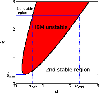
Figure 2. IBM stability as a function of normalised pressure gradient α and magnetic shear  for the cyclone base case (CBC).
Download figure:
Standard image High-resolution image3.2. Gyrokinetic analysis
We examine the KBM and other microinstabilities using
GS2
, which numerically advances the linear electromagnetic gyrokinetic-Maxwell equations in the local limit, with  and
and  fluctuations included, and a Fourier transform being applied in the two dimensions perpendicular to the equilibrium magnetic field (x and y in
GS2
notation; the radial and binormal directions respectively). The equations [24] and the algorithms used to advance them [25] are discussed extensively elsewhere so are not covered here. In this work we will find the complex frequency
fluctuations included, and a Fourier transform being applied in the two dimensions perpendicular to the equilibrium magnetic field (x and y in
GS2
notation; the radial and binormal directions respectively). The equations [24] and the algorithms used to advance them [25] are discussed extensively elsewhere so are not covered here. In this work we will find the complex frequency  (where ω is the real frequency and γ the growth rate) of the dominant mode as a function of
  . ky
is the binormal wavenumber and kx
the radial wavenumber evaluated at the outboard midplane; both are normalised to a 'reference' gyroradius, for which we use the proton thermal gyroradius of the surface,
. ky
is the binormal wavenumber and kx
the radial wavenumber evaluated at the outboard midplane; both are normalised to a 'reference' gyroradius, for which we use the proton thermal gyroradius of the surface,  where
where  is the proton mass and
  the proton gyrofrequency, with
  the reference magnetic field (the toroidal field at the location of the magnetic axis). We will find it helpful to substitute
  with
with  since Ω is periodic in θ0. We will also connect
  to toroidal mode number
  where A is a weakly varying function of ψN
.
where A is a weakly varying function of ψN
.
The gyrokinetic-Maxwell equations used here assume negligible plasma rotation. In reality, sheared rotation in tokamak plasmas does exist and can stabilise microinstabilities [26]. To gauge the magnitude of this effect, we estimate the Hahm–Burrel shearing rate  [26] by calculating the
  flow arising from the diamagnetic flow in the equilibrium. That is, we estimate the
  flow shear from the balance of electric field and pressure gradient forces in the equilibrium, in the absence of externally driven rotation (as expected for reactor-grade tokamak plasmas). The method for this (similar to that used by [27]) is described in appendix
The results presented here simulate a kinetic electron species and a single ion species with a mass of 2.5 times the proton mass; this effectively simulates a deuterium-tritium (DT) plasma with equal densities of isotopes. Collisions are ignored in this work.
Some discussion is given to numerical parameters, impurities and collisions in appendix  ∼1 over most of the plasma (
 ∼0.9). Near the edge (
 ), collisionality becomes more important and the strong shaping presents challenges to the calculation of
GS2
's θ grid; these edge results should therefore be interpreted qualitatively, rather than quantitatively. Suprathermal α particles were included in the equilibrium calculations, but in the gyrokinetic simulation they were incorporated into the ion species by increasing
), collisionality becomes more important and the strong shaping presents challenges to the calculation of
GS2
's θ grid; these edge results should therefore be interpreted qualitatively, rather than quantitatively. Suprathermal α particles were included in the equilibrium calculations, but in the gyrokinetic simulation they were incorporated into the ion species by increasing  and ensuring the kinetic profiles matched the prescribed pressure gradient while maintaining
  and
and  . The kinetic role of suprathermal α particles would be an interesting area of future research.
4. Stability properties of the negative triangularity equilibrium
In the '−ve tri' equilibrium, we find that the second stability is blocked for the entire plasma ( ) and
) and  (figure 3). As a result, the equilibrium is ideal MHD ballooning unstable over the core. In the pedestal, α strays into the second stable region (
 ), coinciding with a sharp drop in the normalised gyrokinetic growth rate
  (lower plot). This supports the picture (validated in section 6.1) that, where the plasma is IBM-unstable, long-wavelength KBMs are the dominant instability. It should be noted that the gyrokinetic growth rate γ is normalised to the thermal velocity associated with the flux surface, so the absolute growth rates have a different (but qualitatively similar) trend.

Figure 3. '−ve tri' equilibrium stability properties vs ψN
. Upper: equilibrium shear ( ) and second stability 'window size' (
 ). Middle: equilibrium pressure gradient (α), marginally IBM-unstable α (
 ); shaded region indicates IBM-unstable plasma parameters. Lower: gyrokinetic growth rate (
 ) for several
  and
and  (solid lines). Dashed line indicates estimated Hahm–Burrel shearing rate
  .
.
Download figure:
Standard image High-resolution imageAt  ∼0.97, there are strongly growing instabilities, as the equilibrium again becomes ballooning-unstable. However, our estimated
  is high in this region, so flow shear (as well as collisions) would likely need be included in simulations to give a realistic picture of stability.
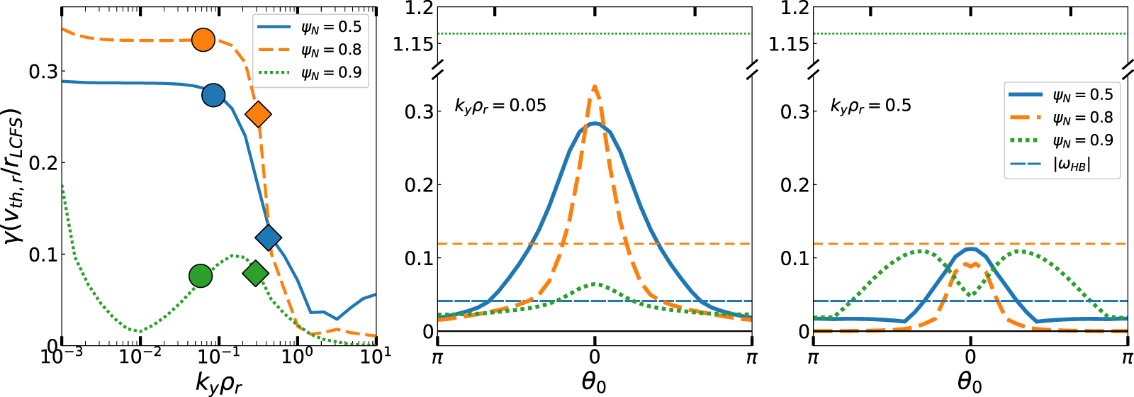
Figure 4 shows  for several values of ψN
. For
for several values of ψN
. For  , the instability spans a wide a range of low
  , suggestive of an 'ideal' KBM, largely governed by ideal MHD physics [17, 18]. These KBMs are also wide in θ0, and thus less easily stabilised by flow shear.
  shows the KBM being less unstable for modes with
  ∼0.1, before the onset of a tearing parity mode at
  ∼0.01.
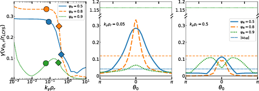
Figure 4. Gyrokinetic growth rate γ for several flux surfaces for '−ve tri' equilibrium. Left:  for
for  , (
, ( and
and  marked with filled circles and diamonds respectively). Middle and right:
  for
for  and 0.5. Estimated Hahm–Burrel shearing rate
  for each surface shown with thin lines.
Download figure:
Standard image High-resolution imageAlthough nonlinear gyrokinetic simulations would be needed to calculate the turbulent fluxes of particles and energy, our linear results indicate that those fluxes would be large. It should be noted that reliable nonlinear results may be difficult to obtain, since electromagnetic nonlinear simulations commonly fail to saturate for equilibria beyond marginal stability [30].
4.1. Second stability access in the negative triangularity regime
Section 4 supports a simple picture: KBM growth rates tracking IBM stability, and likely unacceptably high for steady-state operation. This prompts the question: is the closing of second stability a general feature of negative triangularity STs, or could a configuration exist with second stability access?
To test this we parametrise the  surface using the model developed by Miller et al [31], which provides an analytic description of the flux surface in terms of nine dimensionless parameters ('Miller parameters') (a description of our parametrisation process is given in appendix
  and reduce
  i.e. to close the second stability window and shrink the first stability region. For negative δ, the effect of increasing κ is to increase
  but reduce
  . This is illustrated in figure 5.
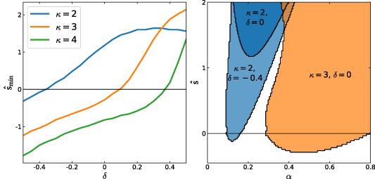
Figure 5. Left: dependence of second stability access window ( ) on elongation (κ) and triangularity (δ) for the
  surface of '−ve tri' equilibrium. Right: IBM unstable regions for
  (light blue),
  (dark blue),
  (orange).
Download figure:
Standard image High-resolution imageThese results indicate that, where ballooning modes are concerned,  is not an attractive option, unless β is sufficiently low that the equilibrium remain in the first stable region. For
  for example,
  , compared with the equilibrium value of
  . Fixing the plasma size, a low-β device would require a large magnetic field. While high temperature superconductors may provide a possible pathway, they present engineering challenges.
It should be noted that the other Miller parameters, such as q, also affect  . A general study of the parametric dependencies of the IBM is beyond the scope of this work, but we note that relatively large changes to the Miller parameters of this surface are required to open second stability at fixed
  . As an example, achieving
  for our negative triangularity scenario requires increasing q from 3.0 to 5.4 with all other parameters kept fixed.
We also explored adjusting the magnitude of the local Shafranov shift parameter,  . This is generally higher in the positive triangularity equilibria than for negative triangularity (e.g. 'high
  ' has 10% greater shift than '−ve tri' at
  ), probably due to the reduced core pressure in the latter, and one may wonder whether this modifies stability. We found that
  decreased (i.e. became more negative) as the magnitude of shift increased from its original Miller-fitted value. Whilst this is not exactly the same as recalculating the global equilibrium with an increased core βN
, this result suggests that attempting to operate at higher β is unlikely to alleviate the problem of second stability access.
decreased (i.e. became more negative) as the magnitude of shift increased from its original Miller-fitted value. Whilst this is not exactly the same as recalculating the global equilibrium with an increased core βN
, this result suggests that attempting to operate at higher β is unlikely to alleviate the problem of second stability access.
5. Stability properties of positive triangularity equilibria
We now consider the positive triangularity equilibria. Consistent with remarks made in section 4.1, we find these have better IBM stability, with  everywhere as shown in figure 6. Despite this, 'low
  ' is unstable near the magnetic axis (
 ∼0.5), illustrating the importance of current distribution (via its effect on q) on ballooning stability. A 'high
  ' is achieved with a hollow current profile, and this is IBM-stable across the plasma.
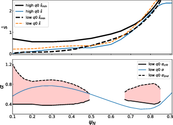
Figure 6. Upper:  and
and  for the positive triangularity equilibria. Lower: α,
  and
and  for the 'low
  ' equilibrium. NB for 'high
  ',
',  for all values of ψN
, so
for all values of ψN
, so  and
and  is undefined.
Download figure:
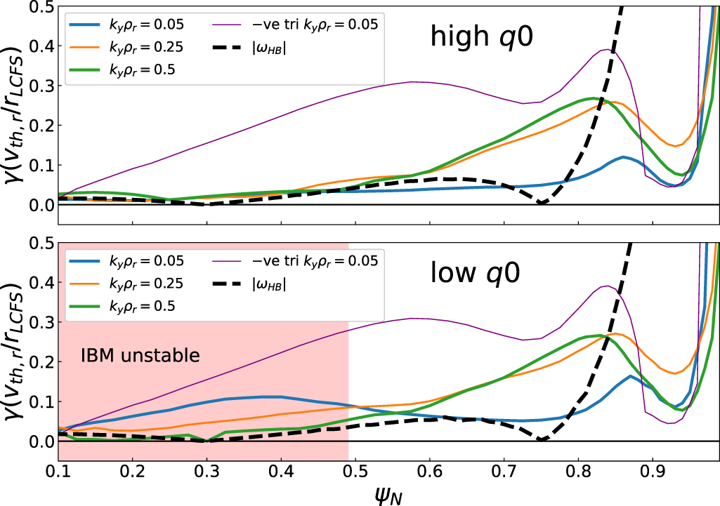
Standard image High-resolution imageThe gyrokinetic  (shown in figure 7) show similar behaviour between 'high
  ' and 'low
  ' for
' for  ∼0.5 (consistent with the similarity of
  ). In this region, instabilities with shorter wavelengths (
 ) are dominant for
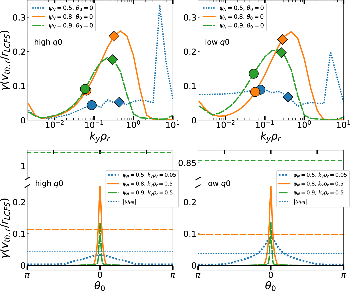
  , peaking near the pedestal top. However, as shown in figure 8,
  is very narrow, and hence highly susceptible to
  shear stabilisation.

Figure 7.
 for 'high
  ' (upper) and 'low
  ' (lower) with
  . '−ve tri' (
 ) shown for comparison (thin purple line). All growth rates normalised to
  for their own flux surface and equilibria. Dashed black line indicates approximate magnitude of Hahm–Burrel shearing rate
  . Shaded region indicates ideal MHD ballooning unstable surfaces.
Download figure:
Standard image High-resolution image
Figure 8. Upper row:  for 'high
  ' (left) and 'low
  ' (right) for several ψN
,
' (right) for several ψN
,  .
.  and
and  marked with filled circles and diamonds respectively. Lower row:
  for selected ψN
,
for selected ψN
,  for 'high
  ' (left) and 'low
  ' (right). Estimated Hahm–Burrel shearing rate
  shown with thinner horizontal lines.
Download figure:
Standard image High-resolution imageHowever,  differs in the core (
 ∼0.5), coinciding with differences in IBM stability. 'low
  ' exhibits a long-wavelength 'ideal' KBM (
 shown in figure 8), consistent with the plasma being on or over the ideal ballooning boundary. 'high
  ' has small but finite γ at long wavelength. Identification of these dominant instabilities is discussed in the following section.
For both equilibria,  is lower than for '−ve tri', unstable over a smaller range of
  (figure 8) and of similar magnitude to
  over much of the plasma. This represents a dramatic improvement in microstability, as a direct result of making the triangularity positive.
6. Instability identification
6.1. Negative triangularity
Here we seek to identify the core and pedestal instabilities in the '−ve tri' equilibrium, by considering 
 for the
  (core) and
  (pedestal) flux surfaces.
We first verify that the dominant instability tracks the IBM stability boundary in  –α space (as shown in figure 9). For both surfaces, the complex frequency Ω tracks the IBM boundary fairly well; γ is high across the unstable region and the frequency is smooth and in the ion diamagnetic direction
1
.
–α space (as shown in figure 9). For both surfaces, the complex frequency Ω tracks the IBM boundary fairly well; γ is high across the unstable region and the frequency is smooth and in the ion diamagnetic direction
1
.
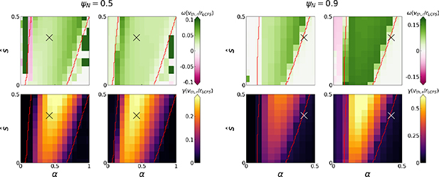
Figure 9. Gyrokinetic  –α plot for the
  (left 4 plots) surface of '−ve tri' equilibrium (
 ) and
) and  (right 4 plots). Top row shows mode frequency ω and lower shows growth rate γ. Left column: fixed β. Right column: fixed gradients. Cross marks equilibrium
  , α.
, α.
Download figure:
Standard image High-resolution imageWe also tested whether the mode was sensitive to α, but not specific contributions ( ,
,  , β). This was done by scanning the quantity
  , in three cases: (1) scaling
  at fixed β, adjusting
  to keep α constant (2) scaling
  at fixed β but keeping
 fixed (such that f changes α, with
  corresponding to
  ) (3) keeping the gradients constant but scaling β. In all cases, we kept the magnetic geometry constant i.e. not changed to be consistent with α.
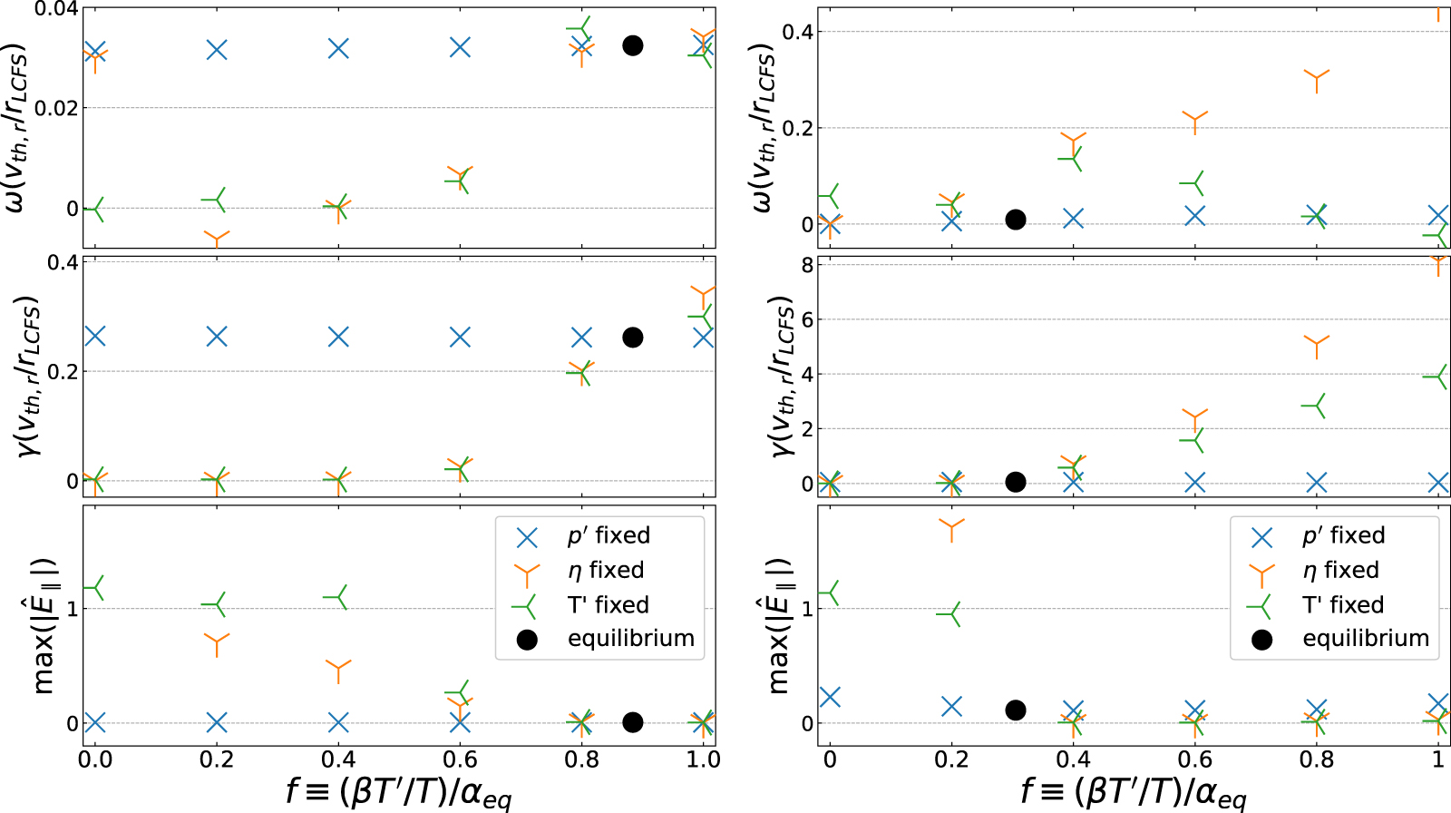
The result of this scan (shown in figure 10) shows Ω and the parallel electric field
max
 max
max
 (normalised to the electrostatic potential φ) are constant with f when α is fixed (case 1). Cases (2) and (3) demonstrate that the kinetic gradients and β are approximately interchangeable in driving the mode (provided
  ). Moreover, the normalised mode structures (
 ,
,  ,
,  ) (figure 11) are virtually identical when f is scanned at fixed α for
  and very similar for
  . This confirms the mode is indeed driven by α.
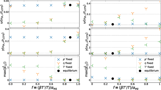
Figure 10. '−ve tri' equilibrium with  . Left:
  . Right:
  . Scanning
  for (1) fixed α and β (blue crosses), (2) fixed η and β (orange (Y)), (3) fixed gradients (green (Y)). Equilibrium value of f shown as black filled circle.
Download figure:
Standard image High-resolution image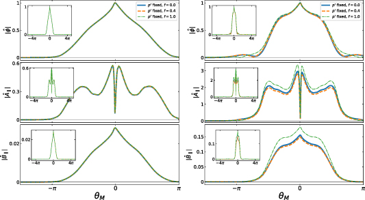
Figure 11. Mode structures for '−ve tri' equilibrium for  (left) and
  (right), with
  as f scanned. θM
is a poloidal coordinate, defined as
as f scanned. θM
is a poloidal coordinate, defined as  , where
  are the geometric elongation and minor radius of the flux surface respectively.
Download figure:
Standard image High-resolution imageWe conclude that the instability observed across the core is an 'ideal MHD'-like KBM, with the following features: (a) γ tracks the ideal MHD boundary well (b) the frequency is in the ion diamagnetic direction (c) the mode has a low parallel electric field  , indicative of MHD-like modes [18] (d) the mode amplitude is greatest in the bad curvature region and (e) has twisting parity (f) the mode preferentially occurs at long wavelength (g) the mode structure and complex frequency are sensitive to α but not to kinetic gradients or β individually. The pedestal, though IBM-stable, has all of the above properties, although γ is more sensitive to
  at long wavelength (figure 4). We speculate this is a 'non-ideal' KBM, destabilised by some kinetic effect(s), allowing it to slightly exceed the ideal boundary.
6.2. Positive triangularity
We repeated this analysis for  for the 'high
  ' and 'low
  ' equilibria. Departures from the ideal MHD stability boundary are seen in
  –α space (figure 12), with the KBM smoothly extending across the IBM boundary into the second stability window. To confirm this smooth transition, we performed a fine scan in
  , keeping α at its equilibrium value (shown in figure 13).
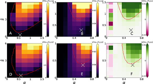
Figure 12. Gyrokinetic  –α plots for the
  surface for
  ,
,  at fixed β. Top row: 'high
  ';
';  over a large range (A), a small range (B) and
  over a small range (C). Bottom row: 'low
  ';
';  over a large range (D), a small range (E) and
  over a small range (F). Crosses indicate equilibrium
  , α.
, α.
Download figure:
Standard image High-resolution image
Figure 13. Upper: ω, γ, max( ) for the
  flux surface for 'high
  ' and 'low
  ' (
' ( ,
,  ) as
) as  is scanned. Equilibrium
  shown by vertical dashed lines and IBM marginal stability by vertical dotted lines.
Download figure:
Standard image High-resolution imageLike the KBMs discussed in section 6.1, the mode has a frequency in the ion diamagnetic direction and twisting parity.  is low, but rises smoothly as
  leaves the IBM unstable region. Scanning
  for 'high
  ' (figure 14), we again find the mode is α-driven. These features were also found for other flux surfaces sampled across the core, and for
  (f scan for
  shown in figure 14). These observations support the conclusion that, although ideal ballooning stable, the dominant long-wavelength instability in these equilibria is a 'non-ideal' KBM.
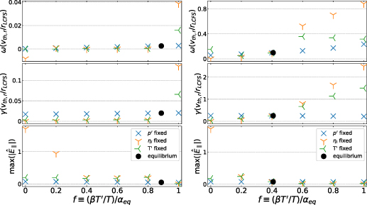
Figure 14. 'high  ' equilibrium; ω, γ,
  as
as  is scanned. Left:
  ,
,  . Right:
  ,
,  .
.
Download figure:
Standard image High-resolution image7. Conclusions
In this work, we have assessed the ballooning stability of three hypothetical ST equilibria, constructed with a commercial power-producing reactor in mind. In all three cases, the normalised pressure gradient α is sufficiently high to exceed the first stable region for ballooning modes; the equilibrium is either in the unstable region, or in the second stability window. In the negative triangularity case, the second stability window does not exist at positive magnetic shear, meaning the plasma is ideal ballooning unstable across the core; this coincides with strongly growing KBMs and indicating that this is unlikely to be a feasible equilibrium in the context of transport. We have considered the dependency of second stability access on shaping parameters, and found that second stability may be obtained either by making triangularity more positive, or reducing the elongation. These point to KBMs prohibiting negative triangularity as an option in commercial STs, unless they can be operated at very high field (which then introduces engineering challenges).
The equilibria with positive triangularity show better stability properties. In these, second stability access exists across the plasma and, provided the on-axis safety factor is not too low, the equilibrium occupies the second stability window across its full radius. Microinstability growth rates are correspondingly low. However, there remains a weakly growing instability with KBM-like properties, namely: pressure-driven, twisting parity, smoothly connecting to the 'ideal MHD' KBM, low parallel electric field and, in some cases, the modes are pervasive at long wavelength. We speculate that the KBM is destabilised by kinetic effects. Being weakly growing, these could feasibly be stabilised by flow shear or may impose a soft β limit on STs. Identifying these effects would be an interesting area of future work, and may be necessary if one wished to build a predictive model of ST H-mode pedestals in a similar manner to EPED [32].
Acknowledgments
The authors are grateful for productive discussions with M Anastopoulos-Tzanis, B Patel, C M Roach, B F McMillan and S Biggs-Fox. This work was supported by the Engineering and Physical Sciences Research Council (EP/L01663X/1) and (EP/R034737/1). This project was undertaken on the Viking Cluster, which is a high performance compute facility provided by the University of York. We are grateful for computational support from the University of York High Performance Computing service, Viking and the Research Computing team. This research used the GS2 version latest commit 142c78781c1bc4c06d234b32fee70eaf100d68e4 (8.1).
Data availability statement
The data that support the findings of this study are available upon reasonable request from the authors.
Appendix A.: Estimation of E × B flow shearing rate
We use an approach similar to that used by Applegate et al [27]. We take the shearing rate as
where B is the magnetic field strength and Φ is the equilibrium electrostatic potential. We estimate Φ by taking the equilibrium force balance
(where p is the ion pressure,  , ʹ denoting a derivative with respect to ψ,
V
the ion flow velocity and
E
the equilibrium electric field), and setting
, ʹ denoting a derivative with respect to ψ,
V
the ion flow velocity and
E
the equilibrium electric field), and setting  . A little manipulation yields
We take B as the field strength on the surface at the location of the magnetic axis.
Appendix B.: Simulation parameters and tests
Since the data used for these simulations is publicly available, we only describe noteworthy parameters here. Their values were chosen to minimise computational cost without compromising accuracy of the simulations; we justify our choice by comparing a selection of  for the three equilibria to higher-fidelity simulations. In particular, the difference in growth rate
  (where γ0 is the growth rate found with our parameters used and
  the growth rate for a higher-fidelity simulation) is used as a figure of merit. In some cases
  is low, resulting in large fractional errors, so here we quote the absolute error (in normalised units of
  ).
).
The parameters governing the parallel coordinate θ are  ,
,  (although it was sometimes necessary to adjust
ntheta
owing to difficulties encountered in
GS2
's
gridgen
module). The former specifies the extent of the simulation domain in ballooning space (
(although it was sometimes necessary to adjust
ntheta
owing to difficulties encountered in
GS2
's
gridgen
module). The former specifies the extent of the simulation domain in ballooning space ( to
to  in our case). This is insufficient to resolve extended microtearing structures which have been seen in high-β equilibria [22], but reasonable for KBMs. Preliminary research did not reveal any extended structures at long wavelength. Comparing
  to
to  we found
  with rms value
  . Comparing
  to
to  , we found
  for
for  and
and  for
for  , reflecting a difficulty in the calculation of geometric quantities in
GS2
for strongly-shaped numerically-prescribed surfaces.
, reflecting a difficulty in the calculation of geometric quantities in
GS2
for strongly-shaped numerically-prescribed surfaces.
The equilibrium data contains density profiles  for electrons, the main ion species (with a mass of 2.5 times the proton mass and
  ), helium ash and two impurity species: tungsten (with typical density
  ) and xenon (
 ) (both assumed fully ionised). Lacking simulated temperature profiles, it was assumed that
  is identical for all species (the effect of fast ions may be an interesting area of future research.) Comparing simulations with the five kinetic species to the 'reduced' simulation with two kinetic species (in which
  to ensure quasi-neutrality), we found
  .
.
Collisions were ignored in the results presented here. Comparing collisionless to collisional simulations, we found  for
for  and
and  for
for  (consistent with the lower temperatures, and hence increased collisionality, near the edge).
Appendix C.: Miller parametrisation
The Miller parametrisation [31] describes each surface by nine dimensionless parameters: aspect ratio A, elongation κ, triangularity δ, the radial derivatives of major radius, elongation and triangularity sκ
, sδ
,  , the safety factor q, normalised magnetic shear
  , and normalised pressure gradient
  . These specify the shape of the flux surface and its poloidal magnetic field:


where R and Z are cylindrical coordinates (with the magnetic axis located at  ),
),  the poloidal magnetic field and θM
a poloidal coordinate ranging from 0 to 2π.
the poloidal magnetic field and θM
a poloidal coordinate ranging from 0 to 2π.
We fit Miller parameters to the numerical SCENE flux surface data as follows. Firstly, the numerical values of R, Z and  for the flux surface of interest are extracted from the SCENE data. R and Z are used to construct
  , a poloidal coordinate defined by
 , where
  is the location of the magnetic axis, and is taken from the SCENE equilibrium. Splines of
  and
and  are used to upsample R and Z, and from this calculate the values for A, r, κ, δ and construct Miller's poloidal coordinate by defining

 is then constructed and fitted to equation (C.3), with fitting parameters sκ
, sδ
,
is then constructed and fitted to equation (C.3), with fitting parameters sκ
, sδ
,  ,
,  (the latter determining q).
The above process yields an estimate of the Miller parameters describing a particular surface. However, it treats the parameters (A, r, κ, δ) on a different footing to (sκ
, sδ
,  , q); calculating the former from R and Z does not guarantee an optimal fit of
  , or indeed of (R,Z) (since most of the R, Z points are ignored.) Therefore, we apply an additional step of simultaneously fitting (
 ,
,  ,
,  ) to (
 ,
,  ,
,  ) allowing all eight parameters to vary freely, using the previously calculated values as initial guesses. This method ensures that
  is treated on the same footing as R and Z, at the expense of allowing (A, r, κ, δ) to deviate from their geometric values.
Finally, the values of  and α are selected. Since
  do not depend on
  , these can be scanned independently in
GS2
.
, these can be scanned independently in
GS2
.
A caveat of the scheme presented above is that for reasons of convenience, we use the numerical equilibrium value of q rather than the value derived from  .
.
Plots of the Miller parametrisation for several flux surfaces for each equilibrium are shown in figure C1.  and (
and ( ) show good agreement between the SCENE data and Miller fit in the core, with slightly worse agreement towards the edge; in particular, the fitted
  for the '−ve tri' has a tendency to artificially peak on the inboard side. Another systematic feature of the fitting is that the elongation tends to be underestimated in the positive triangularity cases and overestimated in the negative triangularity case, with the effect becoming more exaggerated at higher ψN
.
for the '−ve tri' has a tendency to artificially peak on the inboard side. Another systematic feature of the fitting is that the elongation tends to be underestimated in the positive triangularity cases and overestimated in the negative triangularity case, with the effect becoming more exaggerated at higher ψN
.
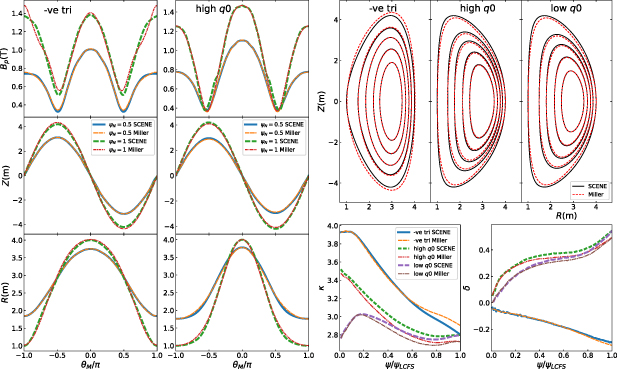
Figure C1. Comparison of numerical equilibria data generated by SCENE to Miller parametrisation. Left: R, Z,  as a function of poloidal coordinate θM
. Right, upper: flux surface shape for
as a function of poloidal coordinate θM
. Right, upper: flux surface shape for  . Right, lower: elongation (κ) and triangularity (δ) vs ψN
; calculated directly from SCENE data and Miller parametrised.
. Right, lower: elongation (κ) and triangularity (δ) vs ψN
; calculated directly from SCENE data and Miller parametrised.
Download figure:
Standard image High-resolution imageFootnotes
- 1
To self-consistently change α, one must scale the simulation value of β and/or the normalised kinetic gradients (
 , ). Both of these choices are shown in figure 9.

