
Abstract
The effects of a short plasma density scale length on laser-driven proton acceleration from foil targets is investigated by heating and driving expansion of a large area of the target rear surface. The maximum proton energy, proton flux and the divergence of the proton beam are all measured to decrease with increasing extent of the plasma expansion. Even for a small plasma scale length of the order of the laser wavelength (∼1 µm), a significant effect on the generated proton beam is evident; a substantial decrease in the number of protons over a wide spectral range is measured. A combination of radiation-hydrodynamic and particle-in-cell simulations provide insight into the underlying physics. The results provide new understanding of the importance of even a small plasma density gradient, with implications for applications that require efficient laser energy conversion to ions, such as proton-driven fast-ignition of compressed fusion fuel.
Export citation and abstract BibTeX RIS

Original content from this work may be used under the terms of the Creative Commons Attribution 4.0 license. Any further distribution of this work must maintain attribution to the author(s) and the title of the work, journal citation and DOI.
1. Introduction
The use of high power laser pulses to accelerate ions to multi-tens-of-MeV energies has been investigated extensively over the past two decades [1]. This has been driven both by exploration of the underpinning physics and by applications of the unique properties of the beams of energetic ions, including for isochoric heating of matter [2], radiographic density probing of materials with micrometre accuracy [3] and to probe highly transient electric and magnetic fields in plasmas with picosecond resolution [4]. These sources may potentially also be applied to address important societal challenges, including in medicine (e.g. for oncology [5, 6]) and energy (e.g. proton fast ignition of fusion targets [7]).
Several laser-driven ion acceleration schemes have been demonstrated experimentally, with the target normal sheath acceleration (TNSA) mechanism [8] being the most widely investigated due to its robustness and the usability of the resulting high quality beams as probes [3, 4]. In TNSA, a high power laser pulse irradiates the front surface of a target foil, generating a plasma. The laser ponderomotive force accelerates plasma electrons from the region of the focal spot forward and they propagate across the target foil to the rear side, where upon leaving the target they establish a charge separation electric field of the order of TVm−1 within a thin (micron-scale) sheath. Atoms at the rear surface are ionised and accelerated by this strong field, in a direction normal to the initial target surface. Protons, which have the highest charge-to-mass ratio, are efficiently accelerated from hydrogen present in surface contaminants. Tens-of-MeV energies are gained, with maximum proton energies (via TNSA) in excess of 85 MeV having been reported [9].
The extent to which the target foil expands during irradiation by the intense laser pulse plays an important role in ion acceleration. Ultrathin foils can expand such that the combination of the decreasing peak electron density and increasing relativistic electron mass leads to the target becoming relativistically transparent [10, 11] to the laser light. This can result in additional electron heating over the expanded plasma, enhancing the TNSA field and thus ion acceleration, in what is termed the break-out afterburner scheme [12, 13]. Energies close to 100 MeV have been achieved via a hybrid acceleration mechanism involving both TNSA and radiation pressure acceleration in ultrathin foils expanding to the extent that relativistic transparency occurs [14]. The maximum ion energy can also be enhanced by self-focusing of the laser light as it propagates within the expanded plasma [15] and properties such as the spatial distribution of the ion beam can also be strongly affected [16, 17].
Even in the case of relatively thick targets for which TNSA is the dominant acceleration mechanism, expansion at either the target front or rear side can strongly influence the properties of the resultant beam of ions. Front surface expansion can strongly affect the propagation of the laser pulse and the energy coupling to electrons [18, 19]. In long scale length (hundreds-of-microns) plasma, the laser pulse can filament leading to energy deposition in lower density regions of the plasma and inefficient coupling to ions, though for an optimum degree of expansion (tens-of-microns) the laser light can self-focus or channel into the dense plasma, increasing the total energy coupling to fast electrons and ultimately to TNSA ions [18]. By contrast, even a small density scale length (Ls
) at the target rear side can strongly affect TNSA. If the initial density profile is not sharp, the sheath electric field becomes weaker, by a factor that scales with Ls
. Mackinnon et al [20] report that a relatively long plasma scale length ( µm) reduces the maximum proton energy by more than a factor of 4. In that study, rear-surface expansion was induced with a second laser pulse of focal spot
  µm (full-width at half-maximum (FWHM)). In later work, Fuchs et al [21] report a gradual decrease in proton energy with increasing Ls
in the range 3–19 µm, and demonstrate that the population of low-to-mid energy range protons is unaffected for
µm (full-width at half-maximum (FWHM)). In later work, Fuchs et al [21] report a gradual decrease in proton energy with increasing Ls
in the range 3–19 µm, and demonstrate that the population of low-to-mid energy range protons is unaffected for  µm. That study used a laser with a relatively small focal spot with
  µm (FWHM) to induce and control the rear surface expansion. Levy et al [22] report on a study involving even smaller Ls
, and measure a factor of 2 reduction in the maximum proton energy for
µm (FWHM) to induce and control the rear surface expansion. Levy et al [22] report on a study involving even smaller Ls
, and measure a factor of 2 reduction in the maximum proton energy for  nm and with
  µm. The spot size of the laser used to induce the rear side expansion is significant because the lateral extent of the expansion also affects the sheath field strength and the refluxing of electrons within the target, which in turn affects the time over which the sheath field is sustained and thus the ion acceleration time [23, 24].
In this article, we present an experimental and numerical investigation of the influence of the plasma density scale length at the target rear side on TNSA proton acceleration. We uniformly heat and pre-expand a large area on the rear surface using laser-accelerated protons (from a separate target). Consistent with previous studies, we measure a decrease in the maximum proton energy with increasing Ls , but in contrast, we measure a decrease in proton number over the full spectral range. We conclude that the latter is caused by a reduction in the sheath field strength at large radii, where lower energy protons originate. The results show the importance of a sharp density gradient not only for the maximum ion energy, but for the overall laser-to-ion energy conversion efficiency, and thus for applications for which that is important, such as proton fast ignition [7] and radioisotope generation [25].
2. Experimental details
2.1. Experimental set-up
The experiment was conducted using the Vulcan laser at the Rutherford Appleton Laboratory in a dual-beam arrangement. A schematic of the experimental set-up is shown in figure 1. Target 1 (T1) refers to the proton-driver target (the target which produces protons for heating) and Target 2 (T2) refers to the main, proton-heated target. These were irradiated using laser beams B1 and B2, respectively. In the first step, shown in figure 1(a), B1 irradiates T1 at an angle of 20∘. Protons accelerated from the front surface of the B1–T1 interaction irradiate the rear side of T2, leading to heating and expansion of the rear surface (for clarity, throughout this article front refers to the laser-irradiated side of the targets and rear refers to the other side). After a variable delay time, and thus T2 heating and expansion time, B2 irradiates T2 at an angle of 40∘, as shown in figure 1(b). The TNSA protons driven by the B2-T2 interaction travel through T1 and are measured using stacked dosimetry film— radiochromic film (RCF) stack 2 (RCF-2). The effects on the T2 proton beam due to T1 and the B1–T1 interaction are minimal for the majority of the spectral components, with a detailed discussion pertaining to this presented in the supplemental material (available online at stacks.iop.org/PPCF/63/114001/mmedia) (with associated [26–32]).

Figure 1. Schematic of the experimental set-up, showing the two steps corresponding to the dual beam interaction. (a) Initial interaction between laser beam 1 (B1) and target 1 (T1), with the rear-surface-accelerated (TNSA) protons characterised using RCF stack 1 and the front-surface-accelerated protons irradiating and heating target 2 (T2). (b) Second interaction, between laser beam 2 (B2) and target T2, which occurs after a controlled delay in the range 30–150 ps relative to the protons from the B1–T1 interaction arriving at the rear of T2. The delay changes the degree of plasma expansion on the rear side of T2.
Download figure:
Standard image High-resolution imageB1 and B2 were separately compressed to temporal durations  1 ps and
  = 8 ps (FWHM), respectively. Both pulses were p-polarised, with wavelength
  1.053 µm and focused using two separate f/3 off-axis parabolic mirrors to a spot size of 5 µm (FWHM). The total energy on-target for B1 and B2 is
  = (63 ± 5) J and
  = (175 ± 15) J, respectively. These parameters correspond to peak laser intensities
  1020 Wcm−2 and
  1019 W cm−2, respectively. Target T2 is a planar Al foil of thickness
  = 20 µm. The material and thickness of T1 (the target used to generate the source of protons for heating) was varied to determine if there were any effects on the main proton beam (from T2) passing through the T1 target bulk, and was either Si of thickness
  = 30 µm or
  = 225 µm; or Al of thickness
  = 10 µm or
  = 200 µm. The protons accelerated from the target front surface of T1 will be largely independent of the target thickness, in contrast to protons accelerated from the target rear. Where relevant throughout this article, the T1 target type is explicitly mentioned.
Two RCF stacks were used to characterise the spatial-intensity distribution and energy spectrum of the beams of protons accelerated from both interactions. These stacks consist of layers of RCF inter-weaved with filter layers of known material and thickness. This enables the spatial profile of the proton beams to be measured at discrete energy bands. Both film stacks were placed 40 mm away from the two targets and angled perpendicular to their respective target normal axes. RCF-1 was used to characterise the beam of protons accelerated from the rear side of T1. The beam of protons from the front side (used to heat T2) could not be measured on every shot and instead the spatial-dose distribution as a function of energy of the proton beam produced at the target rear side was measured as a proxy to monitor changes in the B1-T1 interaction conditions (as might be induced by shot-to-shot variations in the laser parameters). For all data presented in this article, the corresponding spatial-dose distribution and maximum energy of the protons detected with reference RCF stack 1 are comparable. RCF-2 was used to characterise the TNSA proton beam driven by the B2–T2 interaction. The results obtained using RCF-2 are the focus of this investigation. The RCF dose response for all film stacks is absolutely calibrated.
2.2. Characterisation of the heater proton beam
The heating proton beam, driven by front-surface acceleration from the B1–T1 interaction, was characterised in the absence of T2 with an additional RCF stack positioned 60 mm away, and angled parallel to the face of T2. Figure 2(a) shows proton spectra from this reference B1-T1 interaction, for protons accelerated from both the front and rear surfaces. A higher number of low energy protons is accelerated from the front side, which is advantageous for heating the rear side of T2.
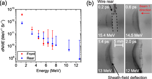
Figure 2. (a) Measured proton energy spectrum of the beam of protons accelerated from the front and rear sides of T1, for Si of thickness  = 225 µm. The error bars are defined by the level of uncertainty in the calibration of the RCF. (b) Example RCF measurements of TNSA protons from T2 probing the spatio-temporal evolution of the sheath-field on T1. The magnification, M, is ×53 and the scale refers to the detector plane (scale on the interaction plane is 1/M times the given scale). The contrast of the images have been scaled independently for clarity. The peak of the laser pulse (B1) arrives at t = 2.0 ps, where 0 ps is the approximate arrival time of the pulse leading edge.
Download figure:
Standard image High-resolution imageComparing all of the laser shots, the difference in flux and maximum energy of the rear-surface proton beam diagnosed with RCF-1, from the B1-T1 interaction, is minimal. All values of the maximum proton energy (εmax ) measured with RCF-1 are in the range εmax = 11-13 MeV. This provides confidence that the heating proton beam is stable and similar for all of the data presented in this article. Regardless, the experimental results and conclusions are always compared to the cold reference cases with the same T1 material.
2.3. Inducing rear-surface expansion via proton heating
The temporal separation between the two interactions was varied to investigate the role of target expansion on proton acceleration. To achieve this, the path length of B2 was changed through careful control of a delay stage with micrometre accuracy. The relative timing of the two beams was initially characterised using a high dynamic range optical streak camera (Hammamatsu C7700), which defined the relative timing of the two pulses (B1 and B2) to within 10 ps. The precision of the relative timing was improved upon by using the proton probing technique. On an initial control shot, B1 irradiates a Cu wire, and B2 irradiates a Cu foil. The protons accelerated from the foil traverse the region of field build-up around the Cu wire, which was charged by the B1-wire interaction, and are diagnosed with an RCF stack. The two beams were timed in such a way that the first protons to arrive at the wire experienced no deflections due to field build-up, while lower energy protons experienced deflections due to the field building up with the rising edge of B1. A similar experimental arrangement was employed previously for proton probing investigations in [33]. Due to the time-of-flight spreading of the broadband proton source, one can determine the coincidence time between the two laser beams with reference to the individual RCF slices. Figure 2(b) shows four example RCF measurements (different RCF samples within the same stack), showing the temporal evolution of the sheath-field from the B1-Cu wire interaction. The dark band seen to evolve over time is the sheath-field, with the degree of deflection experienced by the protons related to the field strength. Close to the peak of the pulse, this field strength is maximised. The time corresponding to t = 0 ps in figure 2(b) is the time of arrival of the leading edge of the pulse. For t < 0, no deflection of protons is observed in the RCF. Employing this technique enabled temporal precision of ∼3 ps.
The two targets were angled at 45∘ with respect to one-another. In addition to optically adjusting the beam path to induce different degrees of target expansion, the two targets were placed a variable distance (L) centre-to-centre from each another, in order to investigate the effect of changes in the proton heating flux. All values of L correspond to either a high or low flux case; L =  mm and L = (
 ) mm for the high and low flux cases, respectively. The timing between the proton beam irradiating T2 and the B2-T2 interaction (th
) was varied in the range
) mm for the high and low flux cases, respectively. The timing between the proton beam irradiating T2 and the B2-T2 interaction (th
) was varied in the range  –150 ps.
  ps corresponds to the time when the highest energy protons have just arrived at B2. A larger value of th
corresponds to a higher degree of target expansion, due to the higher number of incident protons (as a result of the temporal dispersion of the broadband proton source), in addition to the longer expansion time prior to laser-irradiation. Figure 3 provides a guide regarding the time at which protons of a certain energy reach T2, for both values of L. By way of example: for L = 1.2 mm, at
ps corresponds to the time when the highest energy protons have just arrived at B2. A larger value of th
corresponds to a higher degree of target expansion, due to the higher number of incident protons (as a result of the temporal dispersion of the broadband proton source), in addition to the longer expansion time prior to laser-irradiation. Figure 3 provides a guide regarding the time at which protons of a certain energy reach T2, for both values of L. By way of example: for L = 1.2 mm, at  ps protons with energy
  2.5 MeV have arrived; at
  ps, protons with energy
  1 MeV have arrived; and at
  ps, all of the protons with energy ε > 0.5 MeV have arrived. The red curve in figure 3, showing the fractional energy deposited as a function of incident proton energy, demonstrates why a high flux, low maximum energy proton beam is well-suited for heating. Protons with energy ε = 2 MeV will lose roughly half of their energy in T2. Protons of this energy will contribute to target heating far more than protons with ε = 5 MeV, which deposit
  of their energy. With the additional consideration that there are 102 more 2 MeV protons compared to 5 MeV protons, the amount of energy contributing to target heating by the lower energy protons dominates. As shown in figure 2(a), the front surface proton beam contains a significantly higher flux of ε < 4 MeV protons, making this beam favourable for heating.
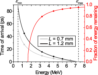
Figure 3. Time of arrival, referred to as heating time (th ) in the main text, as a function of proton energy, for both target separations (L = 0.7 and 1.2 mm). The red vertical axis plots the fractional energy remaining of each spectral component after passing through T2. Zero indicates the proton stops in the material and therefore has deposited all of its kinetic energy. The data points correspond to the spectral components measured in the experiment.
Download figure:
Standard image High-resolution imageIn terms of the proton flux, for ε = 1.2 MeV protons irradiating a target positioned L = 0.7 mm away, the maximum flux is calculated to be  protons mm−2 over a circle of diameter equal to 0.6 mm. For L = 1.2 mm, the maximum flux is calculated to be
  protons mm−2 over a circle of diameter equal to 1.0 mm.
The protons travel deep into the target depositing energy and thus some degree of target heating and expansion at the target front side can be induced by high energy protons. We have modelled the degree of heating and expansion expected and find that this is significantly smaller than the laser contrast-induced scale length (plasma scale length smaller than 0.5 µm) and has a very limited influence on proton acceleration at the rear side. The modelling results and discussion pertaining to this are presented in section 3 of the supplemental material.
3. Experimental results
Figures 4(a) and (b) show representative spectra measured with RCF-2, sampled over the entire proton beam, showing the effect of th
, for L = 0.7 mm (where T1 is 225 µm thick Si) and L = 1.2 mm (where T1 is 30 µm thick Si), respectively. For L = 0.7 mm, higher values of th
consistently reduce the overall number of protons, εmax
and temperature of the distribution. Even for the lowest value of  ps, the number of protons with ε < 5 MeV decreases significantly. For the L = 1.2 mm case, shown in figure 4(b), the effect of increasing th
is less pronounced. Protons with ε = 1.2 MeV do not decrease in number by more than a factor of three over the entire range of th
investigated. However, for all other spectral components, a decrease in number as a function of th
is clearly observed. Similar to L = 0.7 mm, εmax
decreases as a function of th
, but at a slower rate. Comparing the two L cases, the intensity of the heater proton beam is a factor ∼3 less for L = 1.2 mm due to the inherent divergence of the proton beam, and is the core reason why the effects are less pronounced for a given th
. A discussion pertaining to the drop in number of 1.2 MeV protons when comparing the two L-cases, and why this differs, is presented in section 5, where comparisons to the simulation results are made. For each data series, the corresponding plasma scale length
ps, the number of protons with ε < 5 MeV decreases significantly. For the L = 1.2 mm case, shown in figure 4(b), the effect of increasing th
is less pronounced. Protons with ε = 1.2 MeV do not decrease in number by more than a factor of three over the entire range of th
investigated. However, for all other spectral components, a decrease in number as a function of th
is clearly observed. Similar to L = 0.7 mm, εmax
decreases as a function of th
, but at a slower rate. Comparing the two L cases, the intensity of the heater proton beam is a factor ∼3 less for L = 1.2 mm due to the inherent divergence of the proton beam, and is the core reason why the effects are less pronounced for a given th
. A discussion pertaining to the drop in number of 1.2 MeV protons when comparing the two L-cases, and why this differs, is presented in section 5, where comparisons to the simulation results are made. For each data series, the corresponding plasma scale length  is labelled. This is calculated from the simulations in section 4, with the conversion to Ls
as a function of th
and L discussed.
is labelled. This is calculated from the simulations in section 4, with the conversion to Ls
as a function of th
and L discussed.
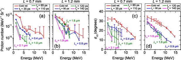
Figure 4. Proton energy spectra for (a) L = 0.7 mm and (b) L = 1.2 mm, as recorded with RCF-2 for the cold (i.e. no B1 but with T1 in place) case, labelled 'cold reference', and several heating times (th ). The error bars are defined by the level of uncertainty in the calibration of the RCF. (c, d) Corresponding measurements of proton beam divergence half-angle for the low and high L cases, respectively. The error bars correspond to the major and minor axis of the proton beam, with a larger error bar indicating a higher degree of ellipticity.
Download figure:
Standard image High-resolution imageFigures 4(c) and (d) shows the measured divergence half-angle ( ) of the proton beams corresponding to the example measurements for which the spectra are shown in figure 4(a) and (b). As expected, for L = 0.7 mm, the change in divergence is more pronounced as a function of th
than for the lower flux case, with the divergence components over the full spectral range reduced for
) of the proton beams corresponding to the example measurements for which the spectra are shown in figure 4(a) and (b). As expected, for L = 0.7 mm, the change in divergence is more pronounced as a function of th
than for the lower flux case, with the divergence components over the full spectral range reduced for  ps. For L = 1.2 mm, the beam divergence reduces compared with the cold target reference case but remains largely unchanged as a function of th
.
ps. For L = 1.2 mm, the beam divergence reduces compared with the cold target reference case but remains largely unchanged as a function of th
.
Figure 5(a) shows how εmax
changes as a function of th
. While the amount of proton stopping is relatively low for all of the T1 target types (as detailed in the supplemental material), small differences in εmax
occurs with different T1 materials and thicknesses. The difference between all species and thicknesses is included in the error bars for the cold T1 reference data point in figure 5(a). In order to take into account the slight variation of proton stopping within the T1 materials, the reduction in maximum proton kinetic energy ( ) with respect to εmax
from the corresponding reference proton beam is plotted in figure 5(b). Comparing the two L-cases, except for the y-intercept, the gradient of the linear trend of
) with respect to εmax
from the corresponding reference proton beam is plotted in figure 5(b). Comparing the two L-cases, except for the y-intercept, the gradient of the linear trend of  as a function of th
is similar. Figure 5(b) indicates that the effect of different values of L on εmax
is to change the heating time required for a specific decrease in maximum energy to be measured. For significantly larger values of L, however, it would be expected that the trend would deviate, due to the time-of-flight dispersion of the heating protons.
as a function of th
is similar. Figure 5(b) indicates that the effect of different values of L on εmax
is to change the heating time required for a specific decrease in maximum energy to be measured. For significantly larger values of L, however, it would be expected that the trend would deviate, due to the time-of-flight dispersion of the heating protons.

Figure 5. (a) Maximum proton energy (εmax
) as a function of heating time (th
) for both values of target separation (L). (b) Energy lost ( ), as a fraction of initial energy through T1. The error bars in εmax
are defined by the energy corresponding to the last RCF layer for which proton signal is measured (lower limit) and the energy of the next RCF layer (upper limit). The boundaries for the cold reference data point (black square) are the maximum and minimum measured εmax
for all of the target species shot cold. The horizontal error bars are a result of the
), as a fraction of initial energy through T1. The error bars in εmax
are defined by the energy corresponding to the last RCF layer for which proton signal is measured (lower limit) and the energy of the next RCF layer (upper limit). The boundaries for the cold reference data point (black square) are the maximum and minimum measured εmax
for all of the target species shot cold. The horizontal error bars are a result of the  ps pulse duration of Beam 2. The corresponding plasma scale length (Ls
) for each L-case as a function of th
is discussed later.
ps pulse duration of Beam 2. The corresponding plasma scale length (Ls
) for each L-case as a function of th
is discussed later.
Download figure:
Standard image High-resolution image4. 1-D radiation-hydrodynamics simulations
In order to investigate the degree of expansion expected in the experiment for a given value of th for both L, the 1-D Lagrangian radiation-hydrodynamic code HELIOS [34] is used. This step is required as it is not possible to optically probe the rear-surface of T2 to determine the rear-surface expansion profile, due to the high density of the expanding plasma.
In HELIOS, material equation-of-state (EOS) and opacity properties are based on the PrOpacEOS tables [34]. HELIOS can inject a proton beam and calculate, via proton stopping, the amount of energy deposited in a material as a function of depth. Proton energy deposition is modelled using a Monte-Carlo algorithm for determining proton trajectories in the target, which enables the temperature and density profiles of the proton-heated target to be calculated over time. Crucially, the intensity of the input proton beam was derived from the RCF measurements of the front-surface-accelerated proton beam, with example data shown previously in figure 2(a). This intensity calculation takes into account the divergence of the beam, L, the duration of the pulse of protons that constitute the beam and energy contained within it, for each spectral component. Important to this investigation is the time of arrival of the various spectral components of the proton beam (with the higher energy protons arriving first). The time of arrival for each spectral component is input into HELIOS, for both L, as shown in figure 3. HELIOS performs a linear interpolation between the tabulated data points, to increase the precision of the simulated beam. Two exponential fits were made to the spectral data for the beam input energy, corresponding to the upper and lower error bars in the dose measurement shown in figure 2(a), with multiple tabulated values entered based on the calculated exponential fits. The same methodology was performed with regards to the beam divergence as a function of energy. For each L case, two sets of simulations were conducted, corresponding to the upper and lower error bars of the calculated intensity. The obtained values delimit the expected target temperature and plasma density profile for each set of parameters. The minimum proton energy (εmin
) was set to 0.5 MeV, as previous measurements using the same laser system showed the energy spectra following an exponential trend down to a minimum energy equal to ε = 0.5 MeV [35]. Protons with ε < 0.5 MeV are far less numerous based on these previous measurements, and are therefore not included in the modelling. The target type was initialised as a 1D slab of Al with thickness  28 µm (28 µm = 20 µm /cos[45∘] to account for the angle between T1 and T2), with a 10 nm H2 layer on each side of the Al target to approximate contaminant layers. Increasing this contaminant layer thickness to 100 nm had no significant impact on the expansion dynamics. The resolution was 2.8 µm and 1.4 nm for the Al and H material, respectively, and the entire target was initialised at room temperature.
Figure 6 shows results from the HELIOS simulations. Figures 6(a) and (b) show the electron density (ne
) as a function of X for a proton-heated  28 µm-thick Al target, for L = 1.2 and 0.7 mm, respectively. X = 0 corresponds to the rear of the target, which is the region the heating protons are initially incident and where the TNSA field is generated in the B2-T2 interaction. The limits of the shaded regions are defined by the maximum and minimum intensity cases, as previously described. The difference in the expansion profile for the two L cases arise due to the differing proton flux at the target surface, and thus differing levels of heating. The temperature profiles within the target are provided in the supplemental material. The plasma scale lengths shown in figure 6(c), as a function of proton heating time, are calculated by fitting the exponential
  , where n0 is the initial electron density. This provides an approximate value of Ls
as a function of both th
and L (i.e.
, where n0 is the initial electron density. This provides an approximate value of Ls
as a function of both th
and L (i.e.  ). The fit is performed over the region from solid density down to where the density profile slope changes markedly, at more than three orders of magnitude lower. The double exponential profile is a result of using an Al target with a H contaminant layer, which expand at different velocities.
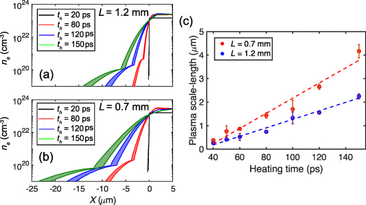
Figure 6. Results from the HELIOS radiation-hydrodynamics simulations. (a) Electron density (ne ) as a function of X for target separation L = 1.2 mm, where X = 0 µm is the initial target rear surface and position of proton incidence. The profile at four given example heating times (th ) are shown and the shaded region is defined by the uncertainty in the input proton beam intensity. (b) Same for L = 0.7 mm. (c) Calculated plasma density scale length as a function of heating time, based on fits to the density profiles, for the two L cases. Ls increases approximately linearly with heating time, as shown by the dashed line.
Download figure:
Standard image High-resolution imageIn figure 7, the maximum proton energy and change in the total laser-to-proton energy conversion efficiency measured in the experiment is plotted as a function of the plasma scale length from the HELIOS simulations, for the L = 1.2 mm case. Both parameters decrease with increasing Ls . The latter corresponds to the fraction of energy remaining (compared with the reference cold target case), contained within the entire measured proton beam over the full spectral range shown in figure 4(b). The simulation results included in these plots are discussed in the following section. Note that a fixed front side plasma expansion profile is assumed, whilst the plasma scale length on the rear surface is varied. This is because the front side profile is defined by the laser pulse temporal-intensity contrast, which is nominally the same for all shots. Any proton heating-induced expansion at the target front side is minimal in comparison, as discussed further in section 3 of the supplemental material.

Figure 7. (a) Maximum proton energy (εmax
) as a function of plasma scale length, as determined from the HELIOS simulations. The black data points correspond to experiment data (for target separation L = 1.2 mm), while the red points correspond to results from the PIC simulations. (b) Fractional change in laser-to-proton energy conversion efficiency ( ) compared to the cold target case. The vertical error bars are defined by the spectral measurements and the horizontal error bars by the accuracy of the fit to the HELIOS simulation results.
Download figure:
Standard image High-resolution image5. 2D particle-in-cell simulations
We next perform 2D particle-in-cell (PIC) simulations of the laser-matter (B2-T2) interaction, using the code EPOCH [36], to investigate whether the density profiles determined from using HELIOS as a function of th and L would result in the measured changes to the proton beam.
In addition to a cold target reference simulation, the density profiles as modelled in Helios for three values of th
and both values of L are used in the PIC simulations. The laser angle of incidence, peak intensity and focal spot diameter were the same as in the experiment for B2, with  fs (FWHM) due to computational constraints. The simulation box was 114 ×108 µm2 with cell size
  nm2, and all boundaries were defined as free-space. The target was initialised as a pre-ionised
  µm slab of Al11+ neutralised by an electron density equal to 100nc
(where nc
is the critical density for λB
). This is less than the density of solid Al to minimise numerical self-heating and the thickness has also been reduced due to the use of a shorter laser pulse. This ensures a number of recirculation passes of the hot electron population within the overdense bulk plasma over the course of the laser pulse interaction, as would be expected in the experiment [37]. The electron beam divergence and the number of achievable recirculation passes is approximately the same for all simulated rear surface scale lengths.
µm slab of Al11+ neutralised by an electron density equal to 100nc
(where nc
is the critical density for λB
). This is less than the density of solid Al to minimise numerical self-heating and the thickness has also been reduced due to the use of a shorter laser pulse. This ensures a number of recirculation passes of the hot electron population within the overdense bulk plasma over the course of the laser pulse interaction, as would be expected in the experiment [37]. The electron beam divergence and the number of achievable recirculation passes is approximately the same for all simulated rear surface scale lengths.
The target front surface was initialised with a  density scale length until the electron density reaches nc
, where Ls
increases to λB
and the pre-plasma profile was truncated at electron density
density scale length until the electron density reaches nc
, where Ls
increases to λB
and the pre-plasma profile was truncated at electron density  . The target rear-surface was initialised using density profiles extracted at several values of th
from the HELIOS simulations, with example density profiles for various th
shown in figures 6(a)–(b). Only the high flux cases were simulated, corresponding to the upper limit of the ne
profile. The
. The target rear-surface was initialised using density profiles extracted at several values of th
from the HELIOS simulations, with example density profiles for various th
shown in figures 6(a)–(b). Only the high flux cases were simulated, corresponding to the upper limit of the ne
profile. The  profile is not varied as a function of target position. As the proton beam transverse size will be significantly larger than the simulation bounds, a 1-D expansion profile can be assumed. The rear-surface of the cold (i.e. reference) target was modelled as a 20 nm layer of protons neutralised by an electron density of
  . The initial electron and ion temperatures were set at 1 keV and 10 eV, respectively, to reduce numerical self-heating effects at early time, and are uniform across the target. The spatially varying temperature induced by proton heating is too low to include in the PIC simulations, but of course the rear-side plasma expansion and thus scale length variation produced by this heating over tens of picoseconds heating time is included. 160 and 20 particles-per-cell (ppc) were used for the electrons and Al11+ ions, respectively. The protons were initialised with 2000 ppc for the cold target and 20 ppc for the heated targets due to the longer expansion profile.
Figures 8(a) and (b) show the proton energy spectra, sampled over the whole simulation domain near the end of each simulation, for L = 0.7 mm and L = 1.2 mm respectively, for given values of th
. Generally, the number of protons over the full spectral range decreases with increasing Ls
. The reduction is significant for values of  µm for both L = 0.7 mm and L = 1.2 mm. Comparing these spectra with the experimental results, shown in figures 4(a) and (b), both the fractional decrease in εmax
(compared to the cold target case) and the reduction in proton numbers with ε > 1 MeV are comparable. The decrease in the number of protons at very low energies measured experimentally in the L = 0.7 mm-case is not reproduced in the simulations. This is likely to result from the susceptibility of low energy protons to the enhanced stopping power of the T1 target (heated by B1) compared to the cold reference case, which is not modelled in the simulations. This is supported by the fact that the same decrease is not observed for the L = 1.2 mm case (figure 4(b)), for which the T1 target used was a factor ∼7 thinner. See the supplemental material for additional discussion of this.
µm for both L = 0.7 mm and L = 1.2 mm. Comparing these spectra with the experimental results, shown in figures 4(a) and (b), both the fractional decrease in εmax
(compared to the cold target case) and the reduction in proton numbers with ε > 1 MeV are comparable. The decrease in the number of protons at very low energies measured experimentally in the L = 0.7 mm-case is not reproduced in the simulations. This is likely to result from the susceptibility of low energy protons to the enhanced stopping power of the T1 target (heated by B1) compared to the cold reference case, which is not modelled in the simulations. This is supported by the fact that the same decrease is not observed for the L = 1.2 mm case (figure 4(b)), for which the T1 target used was a factor ∼7 thinner. See the supplemental material for additional discussion of this.
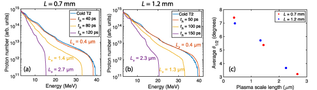
Figure 8. Simulations results using the EPOCH PIC code. (a) Proton spectra for L = 0.7 mm for three values of th
explored numerically. The corresponding Ls
is given beside each spectrum. (b) Same, for L = 1.2 mm. (c) Average divergence half-angle ( ) of the proton beam as a function of Ls
for
) of the proton beam as a function of Ls
for  .
.
Download figure:
Standard image High-resolution imageThe proton beam εmax
and  are plotted as a function of initial Ls
in figures 7(a) and (b), respectively. Similar to the experiment data, both proton beam parameters decrease with increasing plasma scale length, driven by longer heating times. The absolute values in the simulations are higher than experimental due to computational constraints (which limited the peak density and the dimensionality to 2D), but crucially the overall trend is the same. Figure 8(c) shows the average divergence half-angle (
are plotted as a function of initial Ls
in figures 7(a) and (b), respectively. Similar to the experiment data, both proton beam parameters decrease with increasing plasma scale length, driven by longer heating times. The absolute values in the simulations are higher than experimental due to computational constraints (which limited the peak density and the dimensionality to 2D), but crucially the overall trend is the same. Figure 8(c) shows the average divergence half-angle ( ) of protons accelerated with
  . Similar to observations in the experiment, the overall divergence of the higher energy components of the proton beam decreases with Ls
.
. Similar to observations in the experiment, the overall divergence of the higher energy components of the proton beam decreases with Ls
.
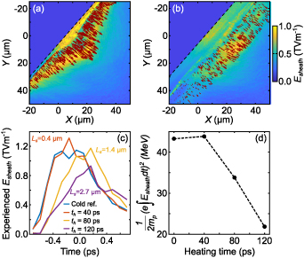
These simulation results indicate that the density scale lengths determined from the HELIOS simulations can produce the measured changes in the properties of the proton beam as a function of  in the experiment. To illustrate the underlying physics, figures 9(a) and (b) show the magnitude of the acceleration electric field (Esheath
) for the cold reference case and
in the experiment. To illustrate the underlying physics, figures 9(a) and (b) show the magnitude of the acceleration electric field (Esheath
) for the cold reference case and  ps with L = 0.7 mm, respectively. This is sampled 0.1 ps after the arrival of the peak of the laser pulse at the target front surface. The magnitude of Esheath
is higher for the case of the cold reference target, which results in higher energy protons compared to the pre-expanded target case. Additionally, the overlaid quiver plot (red arrows) shows that the accelerated protons possess a much higher energy and are predominantly accelerated away from the centre of the rear-surface of the target. As seen in figure 8(c), for increasing Ls
, the average divergence angle of the accelerated protons decreases. This can be seen in the quiver plots, where in figure 9(b) the proton direction appears to align closer to the target normal vector, albeit more randomly distributed, across the expanded sheath field. In figure 9(a), the directionality of the protons appears typical for that of TNSA. This difference indicates that the sheath-field for the expanded targets is flatter than the Gaussian-like TNSA field of the cold target.
ps with L = 0.7 mm, respectively. This is sampled 0.1 ps after the arrival of the peak of the laser pulse at the target front surface. The magnitude of Esheath
is higher for the case of the cold reference target, which results in higher energy protons compared to the pre-expanded target case. Additionally, the overlaid quiver plot (red arrows) shows that the accelerated protons possess a much higher energy and are predominantly accelerated away from the centre of the rear-surface of the target. As seen in figure 8(c), for increasing Ls
, the average divergence angle of the accelerated protons decreases. This can be seen in the quiver plots, where in figure 9(b) the proton direction appears to align closer to the target normal vector, albeit more randomly distributed, across the expanded sheath field. In figure 9(a), the directionality of the protons appears typical for that of TNSA. This difference indicates that the sheath-field for the expanded targets is flatter than the Gaussian-like TNSA field of the cold target.
Figure 9. (a) EPOCH PIC simulation results showing the accelerating electric field (Esheath
) at  ps (where t = 0 ps corresponds to the peak of the laser pulse interacting with the target front side at X = 0), for the cold reference case with no rear-surface expansion. The fields at the front side of the target are removed for clarity. A random sample of 500 macroparticle protons are overlaid, producing a quiver plot that indicates the vector trajectory of the individual protons (at t = 0 ps). (b) Same, for
  ps and L = 0.7 mm (i.e.
  µm). (c) Magnitude of the sheath field (Esheath
) experienced by the highest energy protons as a function of time. The corresponding plasma scale length (Ls
) for each series is stated alongside each plot. (d) Integral of (c), equating to the final energy extracted by the highest energy protons.
µm). (c) Magnitude of the sheath field (Esheath
) experienced by the highest energy protons as a function of time. The corresponding plasma scale length (Ls
) for each series is stated alongside each plot. (d) Integral of (c), equating to the final energy extracted by the highest energy protons.
Download figure:
Standard image High-resolution image
Figure 9(c) shows the magnitude of the sheath field experienced by the highest energy protons, as a function of time, for the cold target case and the three values of th
explored numerically for L = 0.7 mm. This is observed to decrease with increasing  and is due to the maximum sheath strength scaling inversely with Ls
[38]. Figure 9(d) shows the integral of figure 9(c) in time, which equates to the final proton momentum converted to energy. As these energies are comparable to the maximum proton energies in figure 8(a) and in figure 7(a), this provides confidence that the reduction in maximum proton energy measured experimentally is a result of the decreased sheath field at the rear of the target.
and is due to the maximum sheath strength scaling inversely with Ls
[38]. Figure 9(d) shows the integral of figure 9(c) in time, which equates to the final proton momentum converted to energy. As these energies are comparable to the maximum proton energies in figure 8(a) and in figure 7(a), this provides confidence that the reduction in maximum proton energy measured experimentally is a result of the decreased sheath field at the rear of the target.
6. Conclusions
We have shown via experimental and numerical methods that small scale length plasma gradients ( µm) on the rear side of a foil target can have a significant impact on the beam of laser-accelerated protons, especially when induced over the full area of the proton source. The maximum proton energy, laser-to-proton energy conversion efficiency and divergence of the proton beam are all observed to decrease with increasing Ls
. 2D PIC simulations show similar results to those obtained experimentally, and indicate the change in beam properties with Ls
is due to a reduction in the magnitude of the sheath field and a change in the field profile. These results, obtained by heating a large area of the target rear, extend previous investigations for which a reduction in maximum proton energy and proton numbers at high energy only were reported when heating a small region of the target rear surface [21, 22].
µm) on the rear side of a foil target can have a significant impact on the beam of laser-accelerated protons, especially when induced over the full area of the proton source. The maximum proton energy, laser-to-proton energy conversion efficiency and divergence of the proton beam are all observed to decrease with increasing Ls
. 2D PIC simulations show similar results to those obtained experimentally, and indicate the change in beam properties with Ls
is due to a reduction in the magnitude of the sheath field and a change in the field profile. These results, obtained by heating a large area of the target rear, extend previous investigations for which a reduction in maximum proton energy and proton numbers at high energy only were reported when heating a small region of the target rear surface [21, 22].
The results demonstrate the importance of preventing premature expansion of the target rear-surface in TNSA proton acceleration and the impact proton heating can have on the expansion dynamics. However, just as important is the observation that multiple TNSA proton beam properties are strongly altered by variation of the scale length, including the marked reduction in the proton beam divergence. This points to the possibility to develop approaches based on optically-driven controlled changes to the plasma scale length, over the full area of the proton source, to dynamically tune properties of the proton beam, including trading enhancement in one desired property over another, for example, improving beam divergence at the expense of maximum energy.
Data availability statement
The data that support the findings of this study will be openly available following an embargo at the following URL/DOI: https://doi.org/10.15129/2e85773b-35dc-4a86-b01f-243a954172f2. Data will be available from 17 September 2021.
Acknowledgments
We acknowledge the support of staff at the Central Laser Facility. This work is financially supported by EPSRC (Grant Nos. EP/R006202/1, EP/M018091/1 and EP/K022415/1) and used the ARCHER and ARCHIE-WeSt high performance computers, with access to the former provided via the Plasma Physics HEC Consortia (EP/R029148/1). EPOCH was developed under EPSRC Grant No. EP/G054940/1. This work was also performed using resources provided by the Cambridge Service for Data Driven Discovery (CSD3) operated by the University of Cambridge Research Computing Service (www.csd3.cam.ac.uk), provided by Dell EMC and Intel using Tier-2 funding from EPSRC (EP/P020259/1), and DiRAC funding from the STFC (www.dirac.ac.uk). This project has received funding from the European Union's Horizon 2020 research and innovation programme under Grant Agreement No. 871124 Laserlab-Europe.
Prof. David Neely sadly passed away before this work was published. David was a very creative scientist who introduced novel ideas to a wide range of laser-plasma interaction topics, including the development of laser-driven ion acceleration and the use of laser-accelerated protons to heat dense matter. He is deeply missed as a great colleague, mentor and friend.