

Abstract
Extreme ultraviolet radiation from a high harmonic source has been used to measure the free-free attenuation coefficient and real refractive index of warm dense aluminium, with sample conditions of near solid density and temperature of 0.9 ± 0.23 eV. These were compared to results from the literature, where the measured attenuation coefficients showed some consistency with the modelling and existing data from a previous experiment. The absolute values of the attenuation coefficient were found to reside between the different sets of models for the warm dense matter (WDM) attenuation coefficient, and were found to be more in line with modelling and measurements of the cold opacity from the literature. Novel measurements of the real refractive index of WDM were also achieved—while ambiguity makes these measurements consistent with all the models, they prove useful as a proof-of-concept for future WDM studies.
Export citation and abstract BibTeX RIS

Original content from this work may be used under the terms of the Creative Commons Attribution 4.0 license. Any further distribution of this work must maintain attribution to the author(s) and the title of the work, journal citation and DOI.
1. Introduction
Warm dense matter (WDM) is a regime of matter that is of great interest to many experimental and theoretical researchers, as it resides in a middle ground between solid-state physics and plasma physics and is still the topic of much debate. It is of importance as a transient stage of inertial confinement fusion, and the centres of large planets are believed to be in a state of WDM [1–3]. While the basics of solid-state and plasma physics are well understood, warm dense matter is much more difficult to study due to it having too high a temperature for solid-state physics principles to apply (as thermal kinetic energy effects are treated as perturbations on a fixed repeating lattice), but too dense for plasma physics to accurately describe it (as short-range Coulomb effects are treated as a perturbation on thermal motion and long-range Coulomb effects such as plasma waves).
More specifically, much of the difficulty in modelling WDM comes from the presence of strong electron-ion or ion-ion coupling, degeneracy effects and partial ionisation. This makes computing properties which depend on the microscopic state, such as the thermal and electrical conductivities, difficult. However, while microscopic properties of WDM such as the ionisation, degeneracy and ion-ion coupling can be prohibitively difficult to measure directly, these properties directly affect macroscopic properties. One such property is free-free absorption of extreme ultraviolet (XUV) radiation—this is studied here as we can separate this absorption process from other processes, allowing easier comparison with theory. The other prominent absorption process in the XUV region is free-free collisional absorption. For photons below about 11 eV, the light is below the critical density and does not penetrate the foil. At higher than 70 eV bound-free photo-ionisation would be strong and dominate the absorption. While this measurement is challenging in cold matter and exceedingly difficult for WDM, it can provide an important benchmark for WDM physics calculations.
Several different approaches have been used to calculate absorption of XUV radiation in WDM. For example, Vinko et al, following from the treatment of Ron and Tzoar cast their treatment in the form of the dielectric constant which includes the electron fluid part, with local field corrections and a second order correction for the electron-ion interaction that includes the ion-ion structure factor. They use an empty core electron-ion potential with a cut-off radius chosen to fit cold experimental data and a bare Coulomb potential beyond this [4, 5]. Iglesias starts from the classical Kramers result corrected by a Gaunt factor to account for quantum mechanical correction and degeneracy, including multiple collisions and collective effects that are important around the plasmon frequency. The electron-ion potential is given in the form of a screened Coulomb potential, with Z = 3 assumed, outside of short-range frozen core, where the screening length is for a finite temperature electron fluid. The effect of ion-ion correlation is not included in the model, but was estimated by the author to be not significant for the cases considered [6, 7]. In Hollebon et al a DFT model is used in which the Kubo–Greenwood formula for the dynamic electrical conductivity gives the the dielectric function. Corrections are made to account for features not included in the DFT treatment, including local field corrections for the electron fluid and allowing for changes of the exchange-correlation potential for a time dependent process [8]. Shaffer et al also use the Kubo–Greenwood with an average atom model for ionisation, to calculate conductivity and the Kramers–Kronig relation to determine the refractive index and thus opacity [9].
The results give a range of predictions for a given photon energy, which motivated previous experiments and the experiment described here [10–12]. As we shall see below, our experiment agrees with some calculations, but error bars remain large and further measurements, with a higher shot rate and independent checks on sample conditions, are required for precise discrimination between models.
2. Experiment
Since the theoretical modelling by Iglesias, Hollebon et al and Shaffer et al has assumed a temperature of 1 eV (∼11 600 K) and solid density, it is desirable to generate a sample under similar conditions [6, 8, 9]. Indirect heating using keV x-rays was chosen for its ability to uniformly heat a small sample quickly enough to maintain solid density. The samples in this case are 2 mm × 0.5 mm × ∼10−1 µm aluminium foils (thicknesses varying between 200 and 500 nm) that are expected to have several nm of contaminants on each surface (detailed below). At the time of the experiment, the Vulcan Target Area West laser facility was deemed to be the most suitable for this work due to having a kJ-class long pulse laser system, a 100 J 1.5 ps laser for the XUV probe, and a high degree of flexibility in the layout and configuration of these laser beams.
2.1. Sample heating
Figure 1 illustrates the central part of the experimental layout. Figure 1(a) shows a plan view of the laser target assembly, illustrating the principle of the indirect heating. A small sample of cold (i.e. room temperature and solid density) aluminium is placed between two palladium-coated plastic foils 5 . As these Pd foils are heated by the 6 high energy green heating lasers, they emit L-shell radiation that heats the sample as described below and detailed in Kettle et al [13]. In short, 100 J of green laser light is deposited onto each of two parylene-N-coated palladium foils in ∼200 ps over a ∼200 µm wide focal spot (giving an intensity of ∼1015 W cm−2). Approximately 4% of this energy is converted into L-shell emission lines, these have photon energies between 3 and 3.5 keV. Another 4% was released as soft x-ray quasi-black-body radiation (radiation determined to have a temperature of 170 eV), however the 20 µm 6 plastic substrate of the foils attenuated this component by a factor of approximately 104.
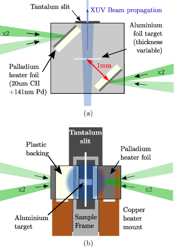
Figure 1. (a) Plan view of target assembly (not to scale). This illustrates the indirect/radiative heating of the sample, and how the weakly diverging XUV beam passes around the sample, before propagating on to a spatially resolving flat-field spectrometer. (b) Side view of target assembly (also not to scale). This shows the XUV beam propagating away from the reader, around the 0.5 mm wide sample. The drop in intensity inside the sample's shadow is used to measure the total opacity, which then allows the absorption coefficient to be calculated.
Download figure:
Standard image High-resolution imageUniformity of heating is achieved, firstly, because the relatively isotropic x-ray sources are significantly separated from the sample, ensuring smooth lateral uniformity across the sample surface regardless of the uniformity of the laser focal spot. Secondly, the absorption length of the L-shell x-rays is much longer than the sample thickness. This latter point ensures uniform deposition through the depth of the sample but limits absorption efficiency to about 10% of incident energy, resulting in heating to about 1 eV. The uniformity (in all three dimensions) is further improved by heating the sample from both sides.
Measuring the temperature using XANES proved to be extremely challenging, so the hydrodynamics simulation code HYADES [14] was used to predict the sample conditions; within ∼100 ps of the start of the heating pulses, this was estimated to have heated the core of the sample to a temperature of 0.9 ± 0.23 eV before it has had time to significantly expand (see figure 2). This is consistent with estimates of the per-atom energy absorption calculated using CXRO's cold opacity data 7 [15]. The uncertainty in the temperature of a single sample is estimated from the uncertainty in the x-ray brightness measurements, taken with a Bragg crystal x-ray spectrometer for each palladium foil. The uncertainty in this brightness is calculated by combining the uncertainties in the crystal reflectivity [16], spectrometer distance measurements and sensitivity of the CCD, giving a relative uncertainty of ∼17%. The shot-to-shot variation in the WDM sample temperature (due to jitter in the laser energy and beam timing) was found to be approximately 26%; this was considered to have a negligible effect on the transmission, as the attenuation coefficient was predicted to have a weak dependence on temperature.

Figure 2. Results from HYADES radiation hydrodynamics simulations of a 300 nm thick WDM sample. (a) Heatmap showing temporal and spatial variation of the electron temperature, (b) snapshot at the time of probing (130 ± 5 ps after heating pulse started) of the spatial distribution along the depth of the sample of its mass density and electron temperature. Grey hatched region highlights the region that is assumed to be the solid density core.
Download figure:
Standard image High-resolution imageThe 'core' is a layer of solid density warm aluminium (∼150 nm thick in this example but will vary depending on the initial sample thickness), highlighted in the grey cross-hatching in figure 2(b). The density and temperature at the time of probing are very uniform and the core is at solid density. However, this uniformity requires the probe to arrive within ±20 ps of the peak of the x-ray heating pulse. While the delay between the heating and probe beams can be measured to ∼10 ps, the temporal jitter of the two optical lasers was approximately 170 ps at the time of the experiment. This meant that most of the data collected could not be used as the sample was either not yet heated or had significantly expanded and thus was no longer near solid density.
2.2. Sample surface contamination
The lower density and temperature aluminium plasma either side of the core is clear here, but hydrocarbon and alumina plasmas from surface contaminants on the sample will also be present. The contaminant layers (before heating) are estimated to be a few nm of CH (believed to be present due to the environment and estimated from their transmission—see section 3.1) on top of ∼4 nm of aluminium oxide on each side of the sample, which is present on any aluminium surface exposed to oxygen [17, 18]. Due to the thinness of these layers, the phase shift caused by the contaminants is small; however, they absorb XUV light much more strongly than aluminium.
This effect was especially noticeable for the cold contaminants, the sum of which are estimated to have a comparable effect on the total sample transmission to 500 nm of Al [19]. Heated contaminants on the other hand are expected to be photo-ionised by the small amount of soft-x-ray (∼102 eV) radiation that passes through the CH filter on the Pd foils, thus greatly reducing the absorption at the 20–30 eV XUV photon energies being studied here. Using the cold C8H8 opacity data from CXRO, the atoms absorb an average of 3 eV of energy each, and even the first ionisation stages of hydrogen, carbon and oxygen are sufficient to stop most of the photoionisation in the 20–30 eV photon energy range [20].
Although the contaminant layer is hard to characterise, the oxide layer is expected to be consistent between samples [21]. HYADES simulations suggest that the lower density heated outer layer consisting of ionised contaminants, oxide, and Al, is consistent between the three heated samples and is not affected by the thickness of the foil.
2.3. XUV probing
Figure 1(b) illustrates the principle of the probing method. High harmonic generation from a gas jet is used to produce the XUV probe beam; in this set-up three harmonics of the ∼1 J 1.5 ps 527 nm probe laser (9th, 11th, and 13th) were visible. These have photon energies of 21.1, 25.9, and 30.6 eV (λ = 59, 48, 40.5 nm), which places them in the lower end of the 15–70 eV range where free-free absorption dominates. Argon was used in the gas jet due to its high efficiency in this harmonic number regime [22]. The probe laser was focussed into the gas with f/100 optics and the jet was 1 m from the sample. This offset allowed the harmonic beam to expand sufficiently to be larger than the sample and thus a shadow of the sample could be produced on the detector. For this regime of XUV radiation and sample size, we are still in the near-field Fresnel diffraction regime and the shadow of the target is, in fact, a diffraction pattern that is modelled by a code we have devised with the sample size, transmission and phase change on traversing the sample as inputs.
This code is based on the description of Fresnel diffraction given in standard texts such as Hecht [23]; an earlier version of this code is detailed by Kettle [22]. In short, Fresnel diffraction is derived from Huygen's principle, assuming that light is diffracting through a slit, or around a barrier, that is much narrower than the propagation distance. The dominant diffraction mechanism in an optical system can be described by the Fresnel parameter F = a2/Lλ where a is the obstacle size, L is the propagation distance of the light and λ is the wavelength. In this experiment, a = 0.5 mm, L = 1 m, and λ = 40–60 nm, giving a Fresnel parameter of F ≈ 5, indicating that Fresnel diffraction is the most appropriate model to use. The code used here is an advancement over the previous code as it can simulate phase shift due to the sample's refractive index. One result of this modelling compared to the measurement is displayed in figure 3(a).
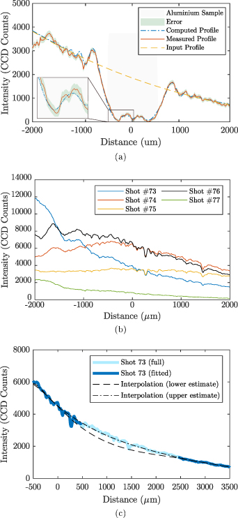
Figure 3. Spatial profile of XUV beams on multiple shots. (a) Profile of shot #137 and associated diffraction modelling. The solid line shows the measured spatial shape of the beam, the dashed line shows the estimate of the beam profile sans shadow and the dot-dashed line shows the results of the diffraction modelling code run with a sample transmission of 11% and a phase shift of 3π rad. The green area surrounding the measurement is the estimated uncertainty in the intensity profile. A zoomed in inset is also shown to make clearer the scale of the error region around the measured beam profile, and the degree of agreement with the diffraction code. (b) Profiles of five consecutive shots from the XUV source commissioning. This demonstrated that in the central region of the beam it is consistently smooth, allowing the 'Input Profile' in figure 3(a) to be estimated by interpolation. (c) Profile of shot #73 from figure 3(b), both the full profile (thick light blue line) and the same profile with some of the points removed (thick dark blue line) and the upper/lower bounds of the spline interpolation used to reconstruct them (dashed black lines).
Download figure:
Standard image High-resolution image3. Data, analysis and results
The result of analysing one of the XUV beam footprints is shown in figure 3(a) (The full dataset is available online [24]). The peaks inside and immediately outside the shadow of the XUV beam caused by diffraction around the sample are clear to see. This makes the analysis non-trivial as we must account for energy diffracted into or away from the shadow region—hence the diffraction code. The code also allows the phase shift caused by the WDM's real refractive index to be measured; the distribution of the light i.e. the shapes of the diffraction peaks, was found to be particularly sensitive to the phase shift of the light passing through the sample. This behaviour was also exploited by Gayer et al to measure the real refractive index of  radiation by measuring the Fresnel diffraction from a knife edge [25].
Note that this analysis required an estimate of the shape of the XUV beam before it reached the sample. While measuring this on each shot was not possible with the experimental configuration used here, the first stage of the experiment was dedicated to optimising the XUV source so that a consistently smooth beam could be produced. The results of this are plotted in figure 3(b). This demonstrates that, while the shape of the beam is not precisely reproducible, the beam is consistently smooth in the region where the sample is positioned. Cubic spline interpolation can then be used to estimate the XUV brightness before the target, as seen in figure 3(a) 'Input Profile'. This interpolation introduces another potential source of error, so rather than fixing the estimate of the input beam profile, upper and lower bounds of the beam profile were drawn, and the diffraction code was allowed to adjust the profile between the two limits. The interpolation was tested on a shot with no sample present where some of the data was removed, representing the typical region that the diffraction features would be observed over. This was found to reproduce the removed data to within error allowed by the interpolation method, as seen in figure 3(c). This highlights the reason for the generous bounds of the interpolation and why the diffraction modelling needed to be able to adjust the input beam profile to fit its output to the measurement.
3.1. Analysis
The measured diffraction profile must be matched to the output from the diffraction modelling code, this requires optimising seven different parameters simultaneously, while allowing for the fact that these parameters are often not independent from each other. The parameters that the code can vary are the pre-sample beam profile, sample width, sample position, XUV transmission and phase shift, source size 8 and sample edge smoothness 9 . It was determined that Bayesian optimisation would be a suitable method for doing so—this is a commonly used method for finding minima of highly non-linear functions that are time-consuming to evaluate.
In short, the optimiser is given an 'objective function' to minimise (in this case, the summed goodness-of-fit parameter), and uses a series of points at different combinations of the parameters to build up a 'surrogate function' that estimates the value of the objective function across the entire parameter space. This is then repeated over a number of points (with the positions of these points guided by the surrogate function with the goal of finding the minimum point) and as a more accurate surrogate function is built up, it quickly converges on the true minimum of the objective function. More detail on how it works can be found in Shalloo et al [26].
In this case, the objective function is the summed goodness-of-fit parameter:

which is calculated for the measured (yi ) and computed (y(xi )) beam intensity profiles with measurement error 10 αi . Each best-fit from the diffraction code is also inspected manually to confirm that it matches the experiment data, with a typical example of such a fit shown in figure 3(a).
The uncertainty in the optimal value of each parameter can then be calculated. While the Bayesian optimisation algorithm does include an uncertainty of the surrogate function, this is not suitable for this use case, so an alternative method must be used. When the goodness-of-fit is calculated as shown in equation (1), the 67% confidence limit for each set of parameters is given by the region where χ2 is between  and
and  . This is more easily visualised in two dimensions, an example of which is shown in figure 4. In this case most of the parameters were fixed, the transmission and phase shift of the shot were varied, and the measured χ2 for each combination was plotted. The minimum and maximum values for each parameter are the extremities of the
  contour, so this example gives a transmission of 9.6 ± 0.5% and a phase shift of (2.96 ± 0.03)π rad. The full explanation for this technique can be found in standard textbooks such as Hughes and Hase [27].

Figure 4. Contour plot showing goodness-of-fit χ2 as a function of phase shift and transmission through sample. The plot contours are plotted for the region where χ2 is between  and
and  .
.
Download figure:
Standard image High-resolution imageHowever, in reality the parameters cannot be assumed to be fixed and optimised independently, for example the assumed sample width has a noticeable effect on the optimum value for the phase shift. Performing a 7D grid parameter scan would be prohibitively computationally expensive, so instead Bayesian optimisation was again used to find a number of random points on the  contour, and the extremities of the range of values found by this method are interpreted to be the error bars for each parameter. It is acknowledged that this is an approximation that will likely underestimate how far the
  contour deviates along each axis but will still capture the relative differences in uncertainty between shots, which is what is required for the next step of the analysis.
3.1.1. Attenuation coefficients.
The effect of the contaminants and surface plasma ('Sample Surface Contamination', section 2) on the absorption was resolved by measuring the change in opacity as the sample thickness was increased. This would have the effect of increasing the thickness of the WDM core while the outer layer of Al plasma and the contaminants would remain the same between shots. The total transmission of a single sample is given by:

where  is the transmission of all the contaminants and surface plasma (assumed to be the same for each sample),
  is the attenuation coefficient of the WDM and
  is the thickness of the sample. Taking log of both sides of equation (2) we see that

so the slope of the plot in figure 5(a) gives us a value for the WDM attenuation coefficien. As indicated earlier, this interpretation relies on assuming that the outer, lower density layers formed largely from the contaminants, oxide and low-density Al, are consistent between shots and that the effect of a thicker sample is simply to increase the thickness of the central WDM core. As discussed in paragraph Sample Surface Contamination in section 2, this assumption (at least for the WDM case) is supported by the hydrodynamics modelling.
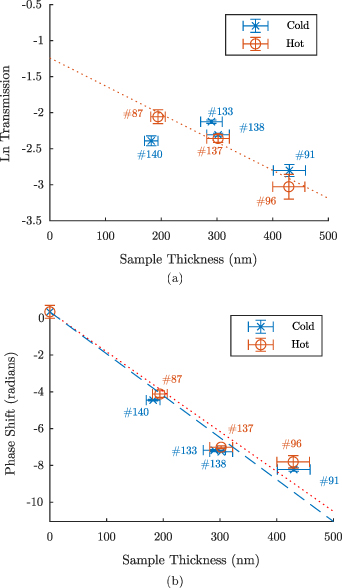
Figure 5. (a) Natural log transmission and (b) phase shift for each sample as a function of sample thickness, for both cold and hot (i.e. WDM) aluminium. The gradients of these plots are used to measure the attenuation coefficient and refractive index of the sample. Note that the phase shift per unit WDM sample thickness is negative (i.e.  ). The horizontal error bars represent the ±5%±5 nm error in thickness quoted by the target manufacturer (e.g. for a 200 nm thick sample, the error will be ±15 nm—see appendix
Download figure:
Standard image High-resolution imageWe can note that whilst this seems to be a justified approach for the WDM case, for the cold case this is not so evident. As seen in figure 5(a) the cold sample transmissions against thickness do not fit to a straight line as well as the WDM sample transmissions. This is believed to be due to older cold targets accumulating highly attenuating hydrocarbon contaminants between being manufactured and having their transmission measured, and the approximate timescale of this accumulation is comparable to measurements by Robinson [17]. This prevented us from obtaining measurements of the cold attenuation coefficient at each harmonic, as there is too much uncertainty in the effect of the contaminants on XUV absorption under these conditions. Contrast this behaviour with that of the heated samples: the three samples had similar variation in age when probed, yet the three points match well to a straight line fit compared to the cold samples. This difference in behaviour is believed to be due to the change in contaminant transmission with ionisation, as discussed earlier 11 .
Measurement of the WDM attenuation coefficient at the 13th harmonic was unsuccessful due to issues with background removal. One of the two heated shots with a sufficiently bright XUV signal (shot #87) was observed to have an abnormally bright and inconsistent background around the 13th harmonic, that was approximately twice the brightness of the measured XUV signal. This meant that the XUV profile for shot #87 at the 13th harmonic could not be reliably estimated and therefore no measurement of the attenuation coefficient was possible (the XUV signal on shot #96 was very weak at the 9th and 13th harmonics). More detail about the background removal process is provided in appendix
The results for the attenuation coefficient measurements are compared with the WDM attenuation predictions and measurements from the literature in figure 6(a), and also with predictions and measurements of attenuation in cold aluminium in figure 6(c) [8, 10, 11]. It is notable that while both material property measurements follow the same trend with photon energy as both Iglesias' and Hollebon's predictions and Hollebon's measurements, the absolute values of the measurements lie below the two sets of predictions and significantly higher than the predictions of the AA-KG model. The comparison with Hollebon's cold opacity measurements in figure 6(c) would suggest that the attenuation coefficient does not change by a large amount as the temperature is changed from 25 meV to 1 eV, however the size of the error bars makes drawing firm conclusions about the temperature dependence of the attenuation coefficient difficult.
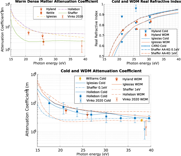
Figure 6. (a) Experimental measurements of attenuation coefficients overlaid on predictions by Iglesias [6], Hollebon et al [8] and Shaffer et al [9]. Opacity data from Kettle et al [10] and Vinko et al [12] are also included. (b) Plausible refractive index measurements overlaid on predictions by Iglesias, Shaffer et al and Henke et al (CXRO) both for cold Al and for WDM [6, 9, 15]. The multiple measurements for the same photon energy come from ambiguity in the phase shift measurements, explained further in the main text in section 3. Note that all the measurements in subfigures (a) and (b) were at the same three photon energies, however they have been slightly offset from each other on the plot for ease of interpretation. (c) Compilation of all the model predictions of attenuation coefficient (both for WDM and cold aluminium), WDM measurements from this work and previous cold Al measurements by Hollebon et al [8], Williams et al [11] and Vinko et al [12].
Download figure:
Standard image High-resolution image3.1.2. Real refractive index.
A similar procedure can be used to extract the refractive index from the data of phase shift against sample thickness, though as the contaminants are  10% of the sample thickness and have a refractive index close to 1, the effect of the contaminants here is expected to be much smaller than on the transmission. The difference between φ0 (phase of the light that passes around the sample) and φ1 (phase of the light that has passed through the sample) Δφ is the quantity measured by the diffraction code. For sample thickness
  and vacuum wavelength λ0, the real refractive index is given by:
 can be easily deduced from the plots in figure 5(b). While measurements were not taken at 0 nm sample thickness, these data points represent the estimated phase shift due to the CH and Al2O3 contaminants, and are based on refractive index measurements from CXRO [15] and Hemmers et al [28]. The effect of the Al2O3 is known to be consistent between shots due to the self-limiting nature of the oxidation process; however the effect of the CH is less certain due to the large uncertainty in thickness (5 ± 5 nm) and composition.
It is notable however, that as the phase shift measurements will be significantly less affected by the uncertainty in the contaminant thickness than the transmission, the shots that were excluded from the cold transmission measurements can be included here. It also means that as the zero-thickness phase shift (i.e. the y-intercept on figure 5(b)) is known to be approximately zero, the refractive index of the WDM at the 13th harmonic can still be evaluated from shot #137. However, one factor here that is not present in the opacity measurements is the cyclical nature of phase shift—as the phase shift through a sample can increase or decrease by multiples of 2π without the diffraction profile changing, many values of the sample phase shift are often possible.
This introduces ambiguity in the refractive index measurements; however, this can be limited by making some assumptions about the possible values for the phase shift. As the WDM is a metal, it has a refractive index less than 1 and as such the phase shift through the sample must be negative. We also expect that the negative phase shift will increase with the sample thickness, so combinations of phase shift and sample thickness where this is not fulfilled can be excluded. Finally, from Kettle's measurements, signal at the 11th and 13th harmonics was observed through the samples at 45∘ incidence, which would be impossible due to total reflection if the refractive index were less than 0.7. Accounting for all these constraints, the plausible values of the refractive index of both WDM and cold Al are plotted in figure 6(b).
While this ambiguity makes drawing firm conclusions about the absolute values of the refractive index difficult, the closeness of the two sets of measurements (WDM and cold aluminium) support the weak temperature variation predicted by both Iglesias [6] and Shaffer et al [9].
4. Summary and conclusions
This technique shows promise, so clearly future work is desirable. Changing the harmonic drive gas would allow higher order harmonics to be created, allowing the higher photon energies in figure 6 to be explored. The VULCAN laser facility now has a much more precise beam timing system, increasing confidence in the measurements as a larger portion of the data collected will have been probed at the appropriate time. The issues with contaminants could also be addressed in future work with the use of a bright UV source to boil the hydrocarbons off the surface of the sample [17]. While the experiment used here contains many enhancements from the previous work, further improvements such as those discussed here would improve the experiment's ability to discriminate between different models. A wider variety of sample thicknesses would also reduce the level of ambiguity in the refractive index measurements.
While Vulcan was the most suitable facility at the time of the experiment, new optical lasers at the European XFEL and LCLS have made them a ideal candidates for this type of experiment. The 100fs XFEL pulse and 25fs optical laser pulse now allow the sample to be heated at not only sub hydrodynamic expansion timescales, but fast enough that the electron-ion equilibration process can be studied using the free-free opacity measurements [11]. The high amount of data that can be collected with such a high shot-rate system would also massively improve the statistics of the measurements, making the overall results far less susceptible to random variation caused by factors such as inconsistent contaminants. While lacking Vulcan's flexibility, the XFEL would also be a far cleaner x-ray source, negating the need for a bright background to be subtracted from the XUV spectrometer signal, as described in appendix
The experimental results along with Hollebon's, Iglesias' and CXRO's predictions are shown in figure 6. These show similar sized error bars to Kettle et al, however we are more confident in the new WDM data due to advances in the experiment design and analysis. Improvements to the HHG source allow a much more reproducible XUV beam to be created, and the development of easy-to-use Bayesian optimisers has allowed much faster and more accurate optimisation of the diffraction code than previously possible [29]. The probe beam is now normal to the sample, which removes the uncertainty caused by refraction in the sample observed in earlier work where the sample was probed at 45 degrees incidence [10]. While the attenuation coefficients predicted by Iglesias and Hollebon are close at the photon energies probed, the measured data is lower than both predictions, and significantly higher than the predictions by Shaffer. The refractive index modelling by Iglesias and Shaffer are also both consistent with the measured refractive indices.
Acknowledgments
This project was carried out as part of EPSRC Grant No. EP/N009487/1. B K is supported by the European Research Council (ERC) under the European Union's Horizon 2020 research and innovation programme (Grant No. 682399).
Data availability statement
The data that support the findings of this study are openly available at the following URL/DOI: https://doi.org/10.17034/5f6b53e1-dd5d-4bc0-ac08-6eb2b0a8941a.
Appendix A.: Burn-through of plastic substrate
Estimates of the broad-band quasi black-body emission were based on results from an earlier experiment [13] that were made using a KAP flat crystal spectrometer to look in the ∼1 keV region where we expect the peak of the broad band soft x-rays to be after passing though the 13 µm CH layer of the earlier experiment. Since we do not expect the heatwave to significantly heat beyond a few microns, it is reasonable to take this estimate for the earlier experiment and add the effect of the additional 7 µm of cold CH for our case, where 20 µm in total was used (we did not get a comparable result in the latest experiment as the flux in the ∼1 keV region was around five times lower). Thus our estimate is based on an experimental measurement that naturally includes the effect of burn-through to the CH layer supplemented by transmission of what we are confident is effectively cold CH.
Appendix B.: Background removal
On all the heated shots a bright background is seen on the XUV spectrometer that is used to measure the spatial profiles of the different harmonic orders in the XUV beam, and hence the diffraction in the XUV beam. This is likely due to hydrocarbon plasma from the palladium heating foils; while having often complex spectral structure, this background is generally spatially smooth (asides from occasional patches of dirt on the sensor, as seen in figure 7), allowing its emission to be interpolated in the region where the XUV signal is measured.
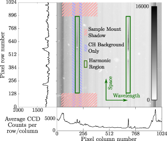
Figure 7. Illustration of the background present on XUV spectrometer when the sample is heated. The raw data from the CCD is shown in the grey-scale image with the spatial and spectral axes of the spectrometer highlighted. The spectral shape of the background is shown in the plot underneath the main image, and the spatial shape is shown in the plot to the left. The defects in the spatial profile of the beam are caused by occasional patches of dirt on the sensor, these are visible in the 2D image as white patches. Three regions surrounding the 9th harmonic ('Harmonic Region') are highlighted—the region containing the harmonic, the regions to the left and right of the harmonic ('CH Background Only', outside of the spectral range of the harmonic) and the regions above and below the XUV signal, where the XUV beam has been blocked by the sample holder ('Sample Mount Shadow').
Download figure:
Standard image High-resolution imageThe process for removing the background is illustrated in figure 7. First the spatial variation of the background is calculated by averaging the intensity either side of the harmonic along the spectral axis (blue cross hatched regions). The spectral variation of the background is calculated using a similar method above and below the harmonic where the XUV signal has been blocked by the stainless steel sample holder (red cross hatched regions). Multiplying these gives the estimate of the background underneath the harmonic, which is then subtracted from the overall signal. The uncertainty in the background removal is gauged from the variation between the harmonics either side or above/below the XUV line—for shots with a similar shape of background either side, the uncertainty is small, for shots with large disagreement between the two backgrounds the uncertainty will be high.
Appendix C.: Uncertainty in sample thickness
The uncertainty in the sample thickness of (±5%)+(±5 nm) is due to the sample manufacturing and characterisation process. The samples are cut from strips of aluminium that are coated onto an NaCl substrate (that is then dissolved away) from a central point. The amount of material deposited on the substrate will drop proportionally to 1/r2 from the source, so the thickness of the strips will vary by up to 5% along their length. An additional 5 nm error is due to uncertainty in the step profilometer that was used to measure the sample thickness.
Footnotes
- 5
For some shots, cold aluminium is also studied. The target configuration remains the same, only the heating laser beams are not fired.
- 6
The absorption of the substrate can be expected to drop slightly as the radiation from the palladium plasma burns through some of the CH, in this case HYADES estimates that about 7 µm of plastic would be burnt through before the end of the laser pulse. However, the soft x-ray flux used here is based on a measurement through the substrate that will already account for this. See appendix A.
- 7
While there is some discussion about the accuracy of this data at low photon energies, it has been extensively studied at the ∼keV region used for this experiment.
- 8
As the harmonic drive laser is focussed with a long f#, the XUV source will be comparable in size to the focal spot. This was simulated by applying a variable width Gaussian blur to the final output of the diffraction model output. It was found to be the order of 100 µm, comparable to the diffraction limit of the laser focus.
- 9
The sample is expected to laterally expand slightly as it is heated, and this expansion was modelled by applying a variable width Gaussian blur to the edges of the simulated sample's opacity. For the cold samples this was found to be close to zero as expected, and the order of 50 µm for the heated samples.
- 10
χ2 is summed across the central region of the beam profile—for the shot shown in figure 3(a) this would be between −1000 and +900 microns over 146 points and outputs a χ2 = 132.5. The measurement error αi is estimated by combining uncertainty in the background subtraction with the standard
 error for discrete counts.
 - 11
Recall that the attenuation for the contaminants is expected to be significantly higher before they are heated, meaning that the transmission of the contaminants by themselves (the y-intercept on figure 5(a)) is expected to be significantly lower than for the WDM. This in turn means that the cold opacity measurements will be significantly more susceptible to variations in the contaminant thickness than hot opacity measurements.
