

Abstract
Reynolds stress is a key facet of turbulence self-organization. In the magnetized plasmas of controlled fusion devices, the zonal flows that are driven by the averaged Reynolds stress modify the confinement performance. We address this problem with full-f gyrokinetic simulations of ion temperature gradient-driven turbulence. From the detailed analysis of the three-dimensional electric potential and transverse pressure fields, we show that the diamagnetic contribution to the Reynolds stress—stemming from finite Larmor radius effects—exceeds the electrostatic contribution by a factor of about two. Both contributions are in phase, indicating that pressure does not behave as a passive scalar. In addition, the Reynolds stress induced by the electric drift velocity is found to be mainly governed by the gradient of the phase of the electric potential modes rather than by their magnitude. By decoupling Reynolds stress drive and turbulence intensity, this property indicates that a careful analysis of phase dynamics is crucial in the interpretation of experiments and simulations.
Export citation and abstract BibTeX RIS
1. Introduction
Since their discovery in numerical simulations as self-organization mediators of magnetized plasma turbulence [1, 2], and since their identification as key players in the saturation of ion-scale turbulence in tokamak plasmas [3], the investigation of the generation of zonal flows is a major research effort aiming at their experimental and theoretical characterization (see the review [4] and references therein). In tokamaks, they correspond to one of the components of the flux surface averaged electric potential, hence resulting in a non-vanishing radial electric field profile. They usually appear at low frequencies as compared to the underlying turbulence, in combination with the zero frequency mean radial electric field—stemming from the radial force balance in the plasma core [5]—and the high frequency geodesic acoustic modes [6] due to magnetic compressibility. By tearing apart turbulence eddies, such sheared flows are regulators of ion-scale turbulence and of the resulting transport [7]. The shear of the radial electric field is suspected to be the main trigger of the transition from low to high confinement regimes in tokamaks [8, 9], and to play an important role in internal transport barriers [10, 11].
From the experimental point of view, the precise role of zonal flows in these bifurcations remains a fruitful and open research area (cf review [12]), in part due to their delicate experimental characterization (cf review [13]). From the theoretical point of view, a critical question is their driving and damping mechanisms. Regarding the former, it was earlier acknowledged that the Reynolds stress is central in this process [14]. There, cross-correlations of the radial and poloidal components of the electric drift fluctuations,  and
and  , may lead to a net momentum transfer from small to large scales, so that zonal flows—the predator—effectively feed on the underlying drift wave turbulence, the prey.
From the perspective of predicting the dynamics and magnitude of the Reynolds stress, and more generally how zonal flows nonlinearly saturate, two important issues are addressed in this paper. The first one deals with the weight of the diamagnetic component. Indeed, it appears that fluctuations of the diamagnetic flow  can also couple to
  and drive a net poloidal momentum at large scale [15, 16]. This term is naturally present in the vorticity equation of fluid codes for plasma turbulence, since the diamagnetic velocity is one of the fluid drifts. In the gyrokinetic framework, it actually emerges from finite Larmor radius effects. To our knowledge, it has received little attention so far. It was reported to be sub-dominant with respect to its electric field and more familiar counterpart shortly after the turbulence overshoot in a gyrokinetic simulation [17]. In the saturated regime of ion temperature gradient-driven turbulence using the GYSELA code with adiabatic electrons [18], we find that it enhances the contribution of the electric drift velocity to the Reynolds stress by a factor of about two. The former characteristics reveal that pressure does not behave as a passive scalar in this case. The second issue addresses the role of the phase that governs the tilt of turbulence eddies. The phase—or tilting—instability has long been known to be a possible mechanism to transform convection into sheared flow in ideal fluids [19]. More recently, the phase curvature was identified as the main component of the Reynolds force in a linear magnetized plasma device [20]. Here, we examine the possibility of driving the Reynolds stress solely from such a tilting instability, independently of the actual behavior of the turbulence intensity. Results from a reduced model of interchange turbulence are used to identify the mechanisms at play in the gyrokinetic simulation. In the latter, the Reynolds stress is found to be well correlated with the time dynamics of the phase—and not with the turbulence intensity. Implications regarding the analysis of experimental data are discussed.
The paper is organized in the following way. Section 2 focuses on the diamagnetic part of the Reynolds stress, detailing its origin and characteristics in gyrokinetic simulations. The role of the phase gradient in the build-up of the Reynolds stress is explored in section 3, both with a reduced model for interchange turbulence and in gyrokinetic simulations. Section 4 closes the paper.
2. Reynolds stress dominated by the diamagnetic contribution
2.1. The two components of the poloidal Reynolds stress
The expression of the poloidal Reynolds stress emerges from the charge conservation equation, which governs the dynamics of the generalized vorticity. Its complete derivation and expression in the gyrokinetic framework, including all radial currents responsible for its time evolution, can be found in [21, 22], and more recently in [23]. In the present work, we only focus on the component governed by the advection by the E × B drift—then putting all other contributions into the right-hand side (RHS) term. Then, the dimensionless gyrokinetic equation reads as follows:

with the Poisson brackets defined by
4
![$\{g,\, f \,\,\} = \frac{1}{r} \left[ \partial_r(g \partial_\theta f\,\,) - \partial_\theta(g \partial_r f\,\,) \right]$](https://content.cld.iop.org/journals/0741-3335/63/6/064007/revision4/ppcfabf673ieqn5.gif) . Here,
. Here,  is the distribution function of the gyro-centers, φ is the electric potential and J[φ] stands for the gyro-average operator applied to φ (strictly speaking, the gyro-average operator is
 ![$\langle J[\phi] \rangle_v$](https://content.cld.iop.org/journals/0741-3335/63/6/064007/revision4/ppcfabf673ieqn7.gif) , with
, with  the integral over the velocity space). For simplicity, the inhomogeneity of the magnetic field is not retained in the first stage, so that grad-B effects leading to turbulence equipartition are not accounted for. B is then simply replaced by B0, which is absorbed in normalizations. The latter are the Larmor radius
  for length scales, the cyclotron period
  for time scale and thermal velocity
  for velocities, where mp
is the proton mass, e is the elementary charge and T0 is a reference temperature. The electric potential is normalized by T0/e. In the long-wavelength limit, J can be approximated by:
for velocities, where mp
is the proton mass, e is the elementary charge and T0 is a reference temperature. The electric potential is normalized by T0/e. In the long-wavelength limit, J can be approximated by:
where µ is the adiabatic invariant, namely the magnetic moment and  . Let us apply the gyro-average operator J to equation (1) and integrate it over the velocity space
  (1)
(1)![$] \rangle_v$](https://content.cld.iop.org/journals/0741-3335/63/6/064007/revision4/ppcfabf673ieqn14.gif) . At this stage, one can use the quasi-neutrality constraint which can be formulated as follows in the Boussinesq approximation:
. At this stage, one can use the quasi-neutrality constraint which can be formulated as follows in the Boussinesq approximation:
where  is the potential vorticity, with
  the flux surface averaged potential. The first term on the RHS is the gyro-center density, and the second one accounts for finite Larmor radius effects in the long-wavelength limit, with
  the transverse pressure. One then obtains up to higher-order terms in
  :
:
Noticing that  , with
  the derivative along the ith Cartesian coordinate in the transverse plane and taking the sum of doubled indexes, equation (4) can be recast as follows:

Equivalently, equation (5) also admits a conservative form:

Here, the Poisson bracket corresponds to the flux of vorticity. Further taking the flux surface average and integrating over the radial direction provides the evolution equation of the E × B poloidal flow  :
:
where the flux-surface averaged Reynolds stress (hereafter simply called Reynolds stress in short) and its diamagnetic component are given by:


The tilde refers to non-axisymmetric components, while  and
and  denote the radial components of the electric and diamagnetic drifts, respectively. As expected, the flux of vorticity is related to the Reynolds stress, which is a restatement of Taylor's theorem [24]. Also, it appears that finite Larmor radius effects, carried by the J operator, lead to an additional contribution to the Reynolds stress, namely
  , as already acknowledged in early publications [15, 16]. Appendix
  is assessed.
Hereafter, π and  are named Reynolds stress and diamagnetic Reynolds stress, respectively.
2.2. Electric and diamagnetic contributions
The structure and dynamics of the total Reynolds stress are explored in a flux-driven gyrokinetic simulation of the GYSELA code [18]. Ion temperature gradient (ITG)-driven turbulence is modeled with an adiabatic electron response.
The simulation is similar to the one already reported in [25] (it is actually a re-run so as to get three-dimensional (3D) data which are required in the present analysis). Its radial domain covers  , with a toroidal limiter treated as an immersed boundary, where relaxation toward a low-temperature Maxwellian is imposed by means of an additional Krook operator [26]. In the simulated scrape-off layer
  , the electron density relative fluctuation is clamped to the floating potential φ = 3Te
/e. The
, the electron density relative fluctuation is clamped to the floating potential φ = 3Te
/e. The  parameter is equal to
  and
and  at r/a = 0.5.
We have also performed the same analysis on another well-resolved simulation for which 3D output data were available. Its radial domain is  , the distribution function driven toward a Maxwellian at the outer edge, characterized by e-folding density and temperature profiles which mimic those expected in the scrape-off layer of tokamak plasmas. Staircases are observed in the fully developed turbulent regime. In this case
  at r/a = 0.5 where the collisionality is
  . Results regarding the present issue are quite similar.
Figure 1 portrays the 2-dimensional (2D) behavior, in space and time, of the flux surface averaged E × B poloidal flow  and of the total Reynolds stress
  . Two main observations can be made. First, the dynamics essentially features avalanche-like events, which draw an array made of diagonal structures. These avalanches propagate both inwards and outwards, roughly at the same speed. Second, there appears to be some correlation between the two images, attesting to the role of the total Reynolds stress in driving zonal flows. Deriving a vorticity equation which is tractable numerically is difficult in the gyrokinetic framework (see, for instance, the expressions proposed in [21–23]). Hereafter, we focus on the total Reynolds stress, bearing in mind its likely dominant contribution to the generation of dynamical corrugated features of the zonal radial electric field.
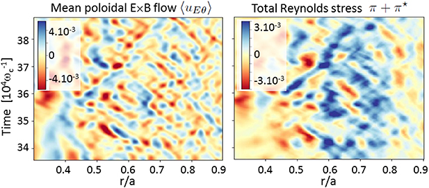
Figure 1. Time derivative of  (left) and Reynolds force (right) versus normalized radius and time. The selected time interval is in the well-saturated turbulent regime.
Download figure:
Standard image High-resolution imageThe respective contributions of the electric and diamagnetic flows to the Reynolds stress π and  respectively are displayed in figure 2. Two main observations can be made. First, π and
  are approximately in phase, with minima and maxima occurring at roughly the same time and radial locations. Second, π* is about twice the value of π. This is shown in figure 3, where each point corresponds to the values of π and
  at any given radial position
  (the radial domain excludes the central region where a non-vanishing heat source is applied and the outer buffer region) and time
  (which corresponds to
  , so well after the overshoot, into the nonlinear saturation phase). The important conclusion is that FLR corrections to the Reynolds stress tensor cannot be ignored, and may even prove dominant in magnitude.
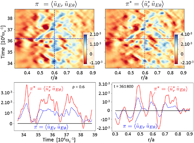
Figure 2. 2D dynamics of π(r, t) (left) and π*(r, t) (right). The color scale is twice for π*. Bottom: time evolution (left) at two different locations and radial profiles (right) at initial and final times.
Download figure:
Standard image High-resolution image
Figure 3. π*(r, t) as a function of π(r, t). Each point corresponds to a value at a given time t and location r. The slope of the dashed line is 2.
Download figure:
Standard image High-resolution imageAt this point, it is worth noticing that this result neither implies nor means that  terms are of order unity; they are actually not, as attested to by the strong cut-off of the turbulence spectra above
  (see e.g. [27]). The phase shift plays a critical role there. Accounting for higher-order terms in
  (
( ) would involve cross-correlations between fluctuations of the electric drift velocity and of high-order derivatives of high-order fluid moments.
The fact that  is found to be larger than π is in marked difference with previous findings. To our knowledge, the only other observation in a gyrokinetic simulation was done by Dimits et al [17]. They report a negligible role of the diamagnetic Reynolds stress in an ITG turbulence simulation for the cyclone base case. Apart from the possible issue with the definition of
  , there are several differences between this simulation and the ones reported in our paper, which may result in these different findings. First of all, the simulation by Dimits is gradient-driven, so that the equilibrium pressure profile is kept constant over time, conversely to our flux-driven simulations. It remains unknown how this constraint may impact the fluctuation dynamics and magnitude of the transverse pressure fluctuations and their gradient, which governs the diamagnetic Reynolds stress
  . Second, cyclone base case gradient-driven simulations are close to the so-called Dimits upshift [28], i.e. close to the nonlinear threshold for turbulent transport. As reported e.g. in [29], they tend to be characterized by a secular growth of zonal flows, rendering early conclusions difficult to interpret. In this respect, and finally, Dimits' result is obtained in the early phase of the simulation: the time window which we have considered for the analysis starts at a time
  roughly equal to twice the final time of the simulation considered by Dimits. In the well-saturated turbulent regime that we consider, Reynolds stress temporal fluctuations are much larger than their almost vanishing mean, conversely to what happens just after the turbulence overshoot in figure 2(a) of [17]. In this same figure, the final state actually looks closer to our finding, especially in the sense that both Reynolds stress components tend to oscillate around a much smaller mean than their standard deviation, and that these standard deviations seem to reach comparable magnitudes, possibly in phase (although this latter point is more difficult to claim from the time traces). Incidentally, the analysis of the second simulation where we have 3D data from the linear phase reveals that the diamagnetic Reynolds stress is always twice as large as the Reynolds stress, even in the early turbulence regime from the overshoot onwards.
2.3. Transverse pressure and potential fluctuations
The approximate proportionality  also indicates that the transverse pressure is not simply advected by the
  flow. Indeed, assuming
  , the linear analysis would lead to the following relation in the 3D Fourier space:
  , with
  the diamagnetic frequency. Here, m and n are the poloidal and toroidal wave numbers,
  is the poloidal wave vector and
  is the time and flux surface average of
  . In this case,
  is expected to be out of phase with respect to
  . This result could have important implications when interpreting experimental data (see e.g. [30]).
In order to look for the origin of the close to zero-phase shift between π and  , the properties of the Fourier components of pressure and electric potential are investigated; see figure 4. Only resonant modes are selected, i.e., such that n + m/q(r)≈ 0, since they are the main contribution to the Reynolds stress. The top panel shows that the amplitudes of the modes peak approximately at the diamagnetic frequency
  (dot–dash black line). The bottom graph is a cut at m =−45. One recovers the ratio of about two between
  and
and  . The relationship between
  and
and  is investigated on a systematic basis in figure 5 which displays all data points of
  as a function of
  ,
,  denoting the real part. These are 3D arrays, functions of ω, m and r. The range of m values has been restricted to
  . The cloud of points does not exhibit any clear structure. Consequently, there is no particular trend indicating some form of correlation. If anything, the sign between both quantities rather appears to be negative. In agreement with the result that π and
  are in phase, one can notice that
  and
and  have the same sign at large amplitude. Since the points are not aligned on the diagonal (black dashed line), this means that the fluctuations of
  are not simply advected by the
  flow.
flow.

Figure 4. Top: amplitude (log scale) of  (left) and
  (right) as a function of poloidal mode number m and frequency ω at r ≈ 175.7. The toroidal mode number is such that
  , i.e. n ≈ −m/q(r). The dotted-dashed line corresponds to the local diamagnetic frequency
  . Bottom: amplitude of
  (blue) and
  (red) at m =−45.
Download figure:
Standard image High-resolution image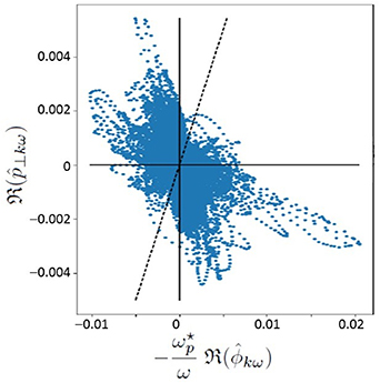
Figure 5.
 as a function of
  . Y stands for
  and X for
  .
.
Download figure:
Standard image High-resolution imageFrom the theoretical point of view, several mechanisms can explain the departure from the passive scalar hypothesis. Within the linear framework and from the fluid perspective, it was already noticed [15] in equation (27) that compressibility could break the simple relationship  . Also, considering the drift-kinetic (i.e., neglecting finite Larmor radius corrections) linear response, one obtains for the Fourier modes
  (
( standing for m, n and kr
, the radial wave vector):
standing for m, n and kr
, the radial wave vector):
with  the frequency-operator associated to the vertical drift
  and FM
the equilibrium Maxwellian distribution function. The brackets
and FM
the equilibrium Maxwellian distribution function. The brackets  denote velocity-space integration. It readily appears that the transverse pressure and electric potential deviate from the above-mentioned simple relationship due to both parallel dynamics
  and compressibility ωd
. The simulation results reported here show that the usual assumption that their effect is negligible does not hold.
and compressibility ωd
. The simulation results reported here show that the usual assumption that their effect is negligible does not hold.
Looking for possible leading terms in the above linear relationship, and/or whether it remains valid in the turbulent regime is certainly an important issue worth addressing in future works.
3. Reynolds stress: critical role of the phase
3.1. Role of phase and amplitude
More insight can be gained into the structure of the Reynolds stress equations (8) and (9) by looking at their expression in the Fourier space. The electric potential φ and transverse pressure  are decomposed in Fourier modes along the periodic directions, the poloidal θ and toroidal ζ angles (no Fourier transform in time is performed there):
with  and
and  the phase of the modes. Then, π and
  can be recast as follows:
and
with  the phase shift between the electric potential and transverse pressure fluctuations.
  denotes the imaginary part, and 'g*' is the complex conjugate of g. Expression (11) highlights that both phase gradient and mode amplitude are key to having a non-vanishing Reynolds stress π, as already emphasized in early works [14]. Conversely,
  can be generated by the gradient of either the phase or the amplitude depending on the phase shift Δϕmn
between the two fields, which then governs the respective weight of each contribution.
can be generated by the gradient of either the phase or the amplitude depending on the phase shift Δϕmn
between the two fields, which then governs the respective weight of each contribution.
3.2. Phase instability in a reduced interchange model
To highlight the role of the phase in the dynamics of the Reynolds stress, we first consider here the reduced nonlinear model proposed in [31] and recalled in appendix  and a single poloidal wave vector denoted ky
. It extends the previous 1D model that features avalanche-like transport events [32] by keeping track of the phase of the density (or pressure since temperature is assumed constant) and electric potential fluctuations. Note that the model is derived in the limit of cold ions, so that the diamagnetic Reynolds stress is not accounted for. On the basis of the results discussed in the previous section, the magnitude of the total Reynolds stress
and a single poloidal wave vector denoted ky
. It extends the previous 1D model that features avalanche-like transport events [32] by keeping track of the phase of the density (or pressure since temperature is assumed constant) and electric potential fluctuations. Note that the model is derived in the limit of cold ions, so that the diamagnetic Reynolds stress is not accounted for. On the basis of the results discussed in the previous section, the magnitude of the total Reynolds stress  —and possibly of the zonal flows—is expected to be enhanced when relaxing this assumption Ti
≈ 0. For the time being, given the considered limit, the poloidal momentum equation reduces to
—and possibly of the zonal flows—is expected to be enhanced when relaxing this assumption Ti
≈ 0. For the time being, given the considered limit, the poloidal momentum equation reduces to  , with
  the poloidal equilibrium flow and x standing for the radial coordinate. The Reynolds stress π takes the simple following form:

with φk
given equation (B.4). As expected from Taylor's identity, the Reynolds force is equal to the vorticity flux:  . An alternative form of π can be obtained by introducing the magnitude and phase of the Fourier mode of the electric potential fluctuations:
 ![$\phi_k(x,t) = |\phi_k(x,t)|\, \exp[i\varphi_\phi(x,t)]$](https://content.cld.iop.org/journals/0741-3335/63/6/064007/revision4/ppcfabf673ieqn106.gif) , with
, with  the phase of the φk
field. The Reynolds stress then reads
the phase of the φk
field. The Reynolds stress then reads

The time evolution of the complex fluctuating fields nk
(or pk
since temperature is assumed constant) and  can be re-expressed in terms of phase and amplitude dynamics as detailed in appendix B.2.
Here, we compare two simulations which only differ by the magnitude S0 of the source term. The values of the various parameters of equation (B.6) have been chosen to be close to the ones used in [31]: Nx
= 256, Lx
= 1, Δt = 2.10−3, ky
= 2π, g = 1 and  . The source term has a Gaussian shape:
with S0∈{20, 30}. The boundary conditions are Dirichlet at x = {0, L} for all fields, except for  at x = 0 where we use Neumann:
  .
.
The time dynamics between the two cases S0 = 20 and S0 = 30 are different, as evidenced on figure 6. For the small source magnitude, fluctuations first grow exponentially in time during the linear phase, and then saturate at a steady-state value. The system reaches a low confinement regime with large amplitude fluctuations and no equilibrium flow. Conversely, for S0 = 30, the system bifurcates toward an improved confinement regime at t ≈ 75. It appears that this transition is due to the generation of an equilibrium flow  .
.
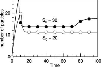
Figure 6. Time evolution of the total number of particles (also proportional to the internal energy since temperature is assumed constant) at two different values of the source magnitude.
Download figure:
Standard image High-resolution imageMost interestingly, it turns out that the build-up of  results from an instability of the gradient of the phase of the electric potential
  . Indeed, as shown on figure 7, the phase gradient starts growing exponentially in time when the magnitude of the fluctuations reaches the first saturated regime. In fact, this governs the exponential growth of the Reynolds stress π up to a second saturation regime, at lower amplitude
  . Conversely,
  does not develop any instability and remains vanishing for S0 = 20, resulting in a vanishing Reynolds stress.
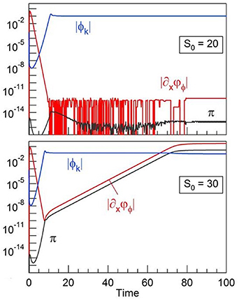
Figure 7. Time evolution of the Reynolds stress π (black), of the gradient of the phase  (red) and of the fluctuation magnitude
  at two different values of the source magnitude.
Download figure:
Standard image High-resolution imageFinding the expression of the growth rate of the phase instability is, however, not obvious. The expression of the time dynamics of the phase gradient  is cumbersome, involving the equilibrium flow
  and the cross-phase between the various fluctuating fields. Yet, one can gain some insight about the physics at work by first noticing that the gradient of the vorticity phase
  evolves according to
  among other terms, equation (B.18):
  . This relation is reminiscent of the main expected effect of the velocity shear on turbulence eddies, namely to increase their radial wave vector kx
:
. This relation is reminiscent of the main expected effect of the velocity shear on turbulence eddies, namely to increase their radial wave vector kx
:  , with
  [4]. During the exponential growth, it appears that all phase gradients exhibit the same growth rate, so that one can also infer
  . Then, accounting for the momentum balance equation with the Reynolds stress, a given equation (14) leads to:

Dirichlet boundary conditions impose  to be concave on average. In fact, with the chosen parameters,
  is broad scale and exhibits a single arch of sinusoid, so that
  is negative everywhere. The positive expression
  then provides a possible explanation for the observed growth rate, which would scale like
 ![$\gamma \approx \sqrt{2}|k_y| \ [\partial_x^2 (|\phi_k|^2)]^{1/2} \sim \sqrt{2}\ |k_yk_x \ \phi_k|$](https://content.cld.iop.org/journals/0741-3335/63/6/064007/revision4/ppcfabf673ieqn131.gif) . In this framework, the phase instability results from the self-reinforced shearing of turbulent eddies (
. In this framework, the phase instability results from the self-reinforced shearing of turbulent eddies ( term) by the Reynolds stress. In the course of the above derivation of the growth rate, we have assumed that the curvature of the Reynolds stress is the dominant term, i.e.
  . Although the detailed analysis of the simulation results reveals that this approximation is marginally valid, it turns out that
  and
and  exhibit a similar shape, hence providing confidence in the qualitative expression of γ.
This instability is also known as the tilting instability, which transforms convection into sheared flow in 2D ideal fluids [19]. It is responsible for the generation of zonal flows by large amplitude drift (or Rossby) waves governed by the Charney–Hasegawa–Mima equation. In this case, it was shown to exist above a finite amplitude threshold of the electric potential [33]. Consistently, the different dynamical regimes characterizing the 1D model are in agreement with the existence of a threshold, with the instability only developing above a critical magnitude  of the driving source term S0, in between
  (cf figure 7). More recently, the possible role of the tilting instability in the bifurcation toward the H-mode in tokamak plasmas has been addressed [34].
In the next section, the evidence of such a phase instability is reported in the saturated regime of flux-driven ITG turbulence.
3.3. The phase gradient and Reynolds stress growth in gyrokinetic simulations
In order to identify the respective role of phase gradient and mode amplitude in the time dynamics of the Reynolds stress π, equation (11) is recast as follows:

where  captures the turbulence intensity.
  —with πmn
defined by the implicit expression
—with πmn
defined by the implicit expression  —is the normalized time-averaged radial profile of the (m, n) spectrum of the Reynolds stress π. This weight aims at discarding contributions
  to the phase gradient
  of (m, n) modes that are far from the resonance condition
  , i.e. n + m/q ≈ 0. The weight Wmn
(r) at r ≈ 180 is displayed on figure 8. The width of Wmn
partly accounts for the fact that GYSELA uses the geometrical angle θ as poloidal coordinate, so that the resonant condition slightly departs from
, i.e. n + m/q ≈ 0. The weight Wmn
(r) at r ≈ 180 is displayed on figure 8. The width of Wmn
partly accounts for the fact that GYSELA uses the geometrical angle θ as poloidal coordinate, so that the resonant condition slightly departs from  . Finally, Δ(r, t) accounts for the mismatch between π and the product
  . Note that
  can be larger than unity due to the use of the weight function in the definition of
  .
.

Figure 8. Weight function Wmn —in logarithmic scale—computed at r ≈ 180, as a function of the toroidal n (x-axis) and poloidal m (y-axis) wave numbers.
Download figure:
Standard image High-resolution imageThe question is whether π is primarily governed by the turbulence intensity  or by the phase gradient
  . To this end, we perform the cross-correlation in time between the Reynolds stress π and
  on the one hand, and π and
  on the other hand. Both are plotted at each radial location in figure 9. These are computed during the same time window of saturated turbulence reported in the previous section 2. It appears that
  exhibits a large correlation with π, up to 0.77 at vanishing time lag. Conversely, at most of the radial positions, the cross-correlation between π and
  remains small or even negative
5
. An example of the time dynamics of these three—rescaled—quantities is plotted on figure 10, at r ≈ 180 (r/a ≈ 0.72). We obtain confirmation that both the increase and decay of π are well correlated with those of the phase gradient
remains small or even negative
5
. An example of the time dynamics of these three—rescaled—quantities is plotted on figure 10, at r ≈ 180 (r/a ≈ 0.72). We obtain confirmation that both the increase and decay of π are well correlated with those of the phase gradient  . Even sometimes, e.g., at t ∼ 35 × 104 and t ∼ 36.7 × 10⁴, π is growing while the amplitude contribution is decreasing. In this case, π is only driven by the growth of the phase gradient.
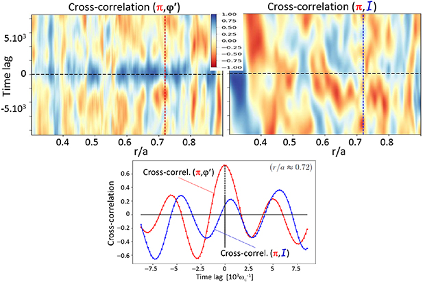
Figure 9. Top panel: cross-correlation in time, at each radial position, between δπ with  (left) and
  (right), with
  . Lower panel: same data at r/a ≈ 0.72.
Download figure:
Standard image High-resolution image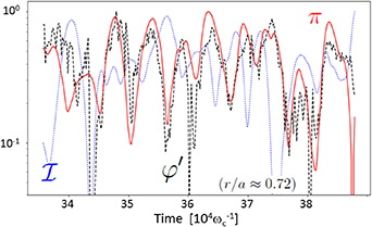
Figure 10. Time evolution of  (red),
  (green) and
  (blue), with
  the fluctuation relative to the maximum at r/a ≈ 0.72.
Download figure:
Standard image High-resolution imageThe critical role of the gradient of the phase in the triggering of a finite poloidal flow has already been acknowledged in the literature [35]. There, from a heuristic model, the authors emphasize that a finite phase curvature alone—i.e. even if turbulence is homogeneous (which translates into  in our notations)—can generate a finite Reynolds force. Such an effect was later reported in experimental measurements in a linear plasma device [20]. The properties of the Reynolds stress in the gyrokinetic simulations that we report here extend these predictions and observations in the temporal space, in the sense that the time evolution of π can be entirely governed by that of
  , even if the turbulence intensity
  remains constant in time.
This result has important implications regarding experimental measurements. Indeed, one of its consequences is that the time dynamics of the Reynolds stress cannot be inferred from that of the amplitude of density—or electric potential—fluctuations only. Indeed, our analysis has shown that π and  are weakly correlated in general, and can event exhibit anti-correlation. In particular, even though the magnitude of the electric potential fluctuations would be roughly constant, this would not necessarily imply that the magnitude of the Reynolds stress—hence possibly of the zonal flows—remains constant either. Conversely, both can actually exhibit opposite trends, as sometimes observed in figure 10. Our results provide the first evidence from gyrokinetic simulations that the time variation of the Reynolds stress is mainly governed by the phase gradient dynamics, rather than by the magnitude of turbulent fluctuations.
4. Discussion and conclusion
The poloidal Reynolds stress is the centerpiece of zonal flow generation. Given the key role of the latter in the regulation of ion-scale turbulence in tokamak plasmas, understanding its structure and dynamics appears essential for at least two reasons. On the one hand, this opens the door to upgraded nonlinear reduced transport models and experimental analyses. On the other hand, this may help tokamak plasma operation by possibly offering controlled access to improved confinement regimes. In this framework, two main results have been reported in this paper, on the basis of the analysis of 3D fluctuation data in gyrokinetic simulations of saturated ITG turbulence (with adiabatic electrons) with the GYSELA code. First, the diamagnetic component of the Reynolds stress is found to be in phase with the one governed by the electric drift, and to be roughly twice as large. This means that the transverse pressure cannot be viewed as a passive scalar in this regime, and that the two components have to be computed to properly quantify the source magnitude of zonal flows. Second, while the Reynolds stress can be roughly split into the product of turbulence intensity times a phase term, it appears that the latter largely dominates its dynamics. Indeed, the phase gradient is strongly cross-correlated with the Reynolds stress, while such a feature is less pronounced with the turbulence intensity. The mechanism is reminiscent of the tilting instability, which is highlighted in a reduced model for interchange turbulence. By decoupling the temporal dynamics of the turbulence intensity from that of the Reynolds stress, this property has profound implications for the interpretation of turbulence experimental measurements.
From the simulation side, the pending questions are twofold. First, what is the role of the diamagnetic Reynolds stress and the phase instability in triggering transport barriers, either a single strong barrier as the H-mode or multiple and comparatively weak as with staircases? Second, how do these features evolve in the presence of kinetic electrons, and for trapped electron mode (TEM) turbulence?
From the experimental point of view, assessing the impact (a) of the phase dynamics and (b) of the diamagnetic drive on the total Reynolds stress is likely more challenging. The former (a) should be accessible via Langmuir probe array measurements at the edge of tokamak plasmas or in other laboratory devices. The latter (b) is more delicate owing to the necessity of measuring both electric potential and pressure fluctuations at the same location. Its importance might be indirectly inferred from the possible imbalance between the divergence of the Reynolds stress  and the time derivative of the zonal flows
  —although other contributions are also expected. In addition, regimes with lower magnitude pressure fluctuations are expected to have a lower Reynolds stress drive, hence reduced zonal flow activity. As a final remark, one can notice that retrieving these characteristics in the hot core of tokamak plasmas—hence in the parameter regime where they have been reported in this paper—may likely prove inaccessible with current diagnostics. Indirect signatures may then be looked for for their validation. In this respect, if the Reynolds stress components are found in numerical simulations to exhibit distinct features in ITG and TEM dominated turbulence, such changes could be detectable experimentally. In any case, our results add to the growing evidence that zonal flow generation is possible even at fixed turbulence intensity.
Data availability statement
The data generated and/or analysed during the current study are not publicly available for legal/ethical reasons but are available from the corresponding author on reasonable request.
Acknowledgments
The authors warmly thank (in alphabetical order) Y Asahi, P H Diamond, N Fedorczak, Z Guo, Ö Gürcan, P Hennequin and D Zarzoso for stimulating discussions, and Ch Passeron for her invaluable support. This work has also greatly benefited from discussions at the tenth Festival de Théorie in Aix-en-Provence (2019, France) and at the first Chengdu Theory Festival (2018, China). This research was supported in part by the National Science Foundation under Grant No. NSF PHY-1748958 during the KITP program on 'Layering in Atmospheres, Oceans and Plasmas' (2021). Last, we are pleased to acknowledge the comments of an anonymous referee, which have lead to the developments found in appendix A. The work has been carried out within the framework of the EUROfusion Consortium and was supported by the EUROfusion—Theory and Advanced Simulation Coordination (E-TASC) initiative under the TSVV (Theory, Simulation, Verification and Validation) 'L-H transition and pedestal physics' project (2019–2020). It has also received funding from the Euratom research and training program. The project has received funding from the European Union's Horizon 2020 research and innovation program under Grant Agreement No. 824158 (EoCoE-II). The views and opinions expressed herein do not necessarily reflect those of the European Commission. This work was also granted access to the HPC resources of TGCC and CINES made by GENCI, and to the EUROfusion High Performance Computer Marconi-Fusion. We acknowledge PRACE for awarding us access to Joliot-Curie at GENCI@CEA, France and MareNostrum at Barcelona Supercomputing Center (BSC), Spain.
Appendix A.:
 from the fluid moment perspective

The aim of this appendix is to make explicit the link between  derived within the gyrokinetic framework (equation (9)) and the fluid moment approach. Especially, the diamagnetic origin of
  is assessed.
In the adiabatic limit where the magnetic field evolves slowly as compared to the cyclotron period and on large scales as compared to the cyclotron radius, the transverse projection of the momentum balance equation stemming from the fluid moment approach can be treated order by order in the small expansion parameter  , with ω and ωci
the characteristic frequency of the problem and the ion cyclotron frequency, and ρi
and R the thermal ion Larmor radius and major radius.
, with ω and ωci
the characteristic frequency of the problem and the ion cyclotron frequency, and ρi
and R the thermal ion Larmor radius and major radius.
At leading order  , the two drift velocities are the electric drift
  and the diamagnetic drift
  :
:
Here, small correction terms proportional to the pressure anisotropy  have been neglected in the expression of the diamagnetic drift. This simplification is even more valid in the present derivation, since these terms originate from the inhomogeneity of the magnetic field, which is neglected here. At next order
  , the polarization drift emerges. Accounting for the gyroviscous cancellation [36], it takes the following form:

Due to the mass scaling, the electron polarization drift can be safely ignored. Now, consider the charge conservation equation  . When neglecting the inhomogeneity of the magnetic field as we did in section 2, the divergence of the diamagnetic current vanishes. Therefore, the divergence of transverse currents reduces to
  , leading to (still using the Boussinesq approximation):
Up to normalization factors, the divergence of the polarization current equation (A.3) turns out to be equivalent to the left hand side of equation (5) within the same approximation of constant magnetic field. Therefore, it readily appears that the pressure terms in the general expression of Reynolds tensor, namely  , originate from the ion diamagnetic drift, which appears in the expression of the polarization drift, equation (A.2). Notice that the charge dependence of the diamagnetic drift—leading to opposite signs for electron and ions—can be safely ignored here, since the polarization drift of ions only is worth being considered.
Last, it should not be a surprise that finite Larmor radius effects within the gyrokinetic framework are related to contributions of the diamagnetic velocity. Indeed, this fluid drift itself actually results from such finite Larmor radius effects, namely the finite excursion of particle trajectories in the transverse plane due to the cyclotron motion.
Appendix B.: Reduced interchange model
B.1. Derivation of the model
We start from the following minimal system for electrostatic interchange turbulence, reduced to two dimensions by considering flute modes  . It involves density n and electric potential φ, coupled together via the continuity and charge conservation equations:


Distances are normalized to the ion thermal Larmor radius  ((x, y)→(x, y)/ρc
), and time to the ion cyclotron frequency
((x, y)→(x, y)/ρc
), and time to the ion cyclotron frequency  (t → ωc
t), with e the elementary charge, T and B being the constant electron temperature (cold ions are considered) and magnetic field. Finally, g ∼ ρc
/R accounts for the average curvature of the magnetic field lines [37]. Each field is split into equilibrium and fluctuating parts. A single poloidal (y direction) mode k is then retained for the fluctuating fields:
(t → ωc
t), with e the elementary charge, T and B being the constant electron temperature (cold ions are considered) and magnetic field. Finally, g ∼ ρc
/R accounts for the average curvature of the magnetic field lines [37]. Each field is split into equilibrium and fluctuating parts. A single poloidal (y direction) mode k is then retained for the fluctuating fields:
Equilibrium (y-averaged) quantities  ,
,  and
and  are real (
 ), while nk
, φk
and wk
are complex fields (
), while nk
, φk
and wk
are complex fields ( ). This approach is in marked contrast with the derivation of [32], where the phase shift between density and potential fluctuations was assumed to be clamped to π/2, hence maximizing turbulent transport. Introducing the equilibrium velocity:

one finally obtains the following 4-field system of equations:
The turbulent particle flux and the Reynolds stress then read:


Alternative forms of the Reynolds force may prove more appropriate for numerical schemes:  .
.
The system (B.6) was initially derived in [31]. Notice that the system proposed in [38] differs from this one by neglecting the radial curvature of the potential with respect to its poloidal one, i.e., it assumes  . In this case, vorticity and potential are in phase. Actually, this latter system proves to be numerically unstable, leading to the transient excitation of fluctuations at spatial scales down to the grid size.
B.2. Amplitude and phase equations
An alternative form of the previous system can be derived by introducing the magnitude and phase of the retained Fourier component k of the fluctuations.
with  and
and  . One further introduces the following phase shifts (for any f, g ∈ n, φ, w):

System (B.6) can then be recast in terms of amplitudes and phases. The equations for the mean quantities read:

Notice that the nonlinear particle flux and the Reynolds stress take the following simple forms:


The time evolution of the fluctuations is given by:
with the following relationship between Aw
and  :
:

The phases are governed by the following equations:
with
Footnotes
- 4
Notice that this definition of Poisson brackets uses an opposite sign convention to that often used in gyrokinetics.
- 5
Noticeably, it appears that the cross-correlation π-
is large when that of π- is lost, e.g. at .

