
Abstract
Turbulence simulations in diverted geometry across the edge and scrape-off layer (SOL) of ASDEX Upgrade are performed with the GRILLIX code (Stegmeir et al 2019 Phys. Plasmas 26 052517). The underlying global (full-f) drift-reduced Braginskii model allows to concurrently study the self-consistent dynamics of the turbulence and the background as well as the evolution of toroidal and zonal flows. Different contributions to the radial electric field are identified. The dominant contribution on closed flux surfaces comes from the ion pressure gradient, due to the diamagnetic drift in the curved magnetic field. Large deviations can be induced, in particular, by the polarization particle flux, leading to zonal flows. The latter are driven by small-scale eddies, but do not exhibit much impact on the overall transport which is driven by ballooning modes at larger scales. Ion viscosity is found to be important in damping poloidal rotation through adjusting of the parallel velocity profile, but not via direct vorticity damping. The zonal flow drive peaks at the separatrix, where a strong shear layer forms due to the sheath-induced counter-propagating SOL flow, allowing for the formation of a transport barrier. The temperature profile across the separatrix is determined by the competition between cross-field transport and outflow in the SOL, the latter being largely controlled by the parallel heat conductivity.
Export citation and abstract BibTeX RIS

Original content from this work may be used under the terms of the Creative Commons Attribution 4.0 license. Any further distribution of this work must maintain attribution to the author(s) and the title of the work, journal citation and DOI.
1. Introduction
The radial electric field and the resulting E × B flows are of central importance in determining magnetic confinement properties of tokamaks [1–3]. In the confined region, the electric field consists of mean-field (neoclassical) contributions as well as of zonal flows generated by the turbulence [4]. The latter result from the interaction of poloidal and radial fluctuations through the Reynolds stress [5], but can also be amplified by the anomalous Stringer drive [6, 7]. A review of zonal flow experiments can be found in [8]. In the scrape-off layer (SOL), on the other hand, in the absence of closed flux surfaces, the electric field is primarily determined by dynamics parallel to the magnetic field, and particularly by the sheath boundary conditions [9, 10]. The interface between closed and open field lines is of central interest. Different mechanisms act on the two sides of the separatrix, leading to electric fields of different signs. Therefore, the electric field changes abruptly across a narrow region and produces strongly sheared E × B flows [11]. This shearing is thought to act as a turbulence suppression mechanism [12, 13], playing a key role in the transition to improved confinement regimes.
To study the formation of the electric field and its back-reaction on turbulent transport, involving both mean and zonal flows, a global (full-f) turbulence model is required. While gyrokinetic models [14, 15] can be more realistic if collisions and electromagnetic effects are taken into account, fluid models are attractive due to their significantly lower computational cost. In the present work, we present theoretical and computational results based on the global version of the drift-reduced Braginskii two-fluid model [16, 17], which is widely used for both direct turbulence simulations [18–21] and simplified transport studies [22, 23]. Although restricted (strictly speaking) in its validity to sufficiently collisional regimes, important insights can be gained. More refined studies may become possible in the future with the help of gyrofluid models employing appropriate closure schemes [24, 25], with full-f formulations currently still under development [26]. The study of the tokamak edge is further complicated by the relatively complex magnetic geometry. As diverted geometry is beneficial for confinement [27–29] and impurity exhaust [30], theoretical and computational studies must adapt to that geometry. A computationally feasible implementation is achieved through the flux-coordinate independent (FCI) approach [31, 32], implemented in the code GRILLIX [33].
In the present study, we report on the first global turbulence simulations in diverted geometry across the edge and SOL of ASDEX Upgrade (AUG), based on the L-mode discharge #36190. The results illuminate many aspects of tokamak edge physics, such as high and intermittent fluctuation levels, up to 10% at the separatrix and of order unity in the SOL. Turbulent vortices in the confined region develop a mean poloidal rotation in the electron diamagnetic drift direction, as the radial electric field balances the ion pressure gradient. Due to the sheath at the divertor, the flow is in the ion diamagnetic drift direction in the SOL. A shear layer develops at the separatrix in which vortices are strained out and decorrelated. Zonal flows are driven by drift waves and damped by the geodesic acoustic mode (GAM). However, this barely affects the ballooning driven transport. Ion viscosity is found to be important for damping poloidal rotation. The competition between perpendicular and parallel transport leads to the formation of a temperature pedestal due to the high parallel heat conduction. Nevertheless, we note that the validity of our fluid model might be yet restricted due to the low collisionality in the plasma edge, and lack of neutral gas recycling and impurities in the SOL.
The remainder of the manuscript is organized as follows. In section 2 we illustrate the key components of the model that lead to the formation of the multi-scale electric field (the full set of equations is detailed in appendix
2. The electric field in drift-reduced Braginskii models
The radial electric field Er in a tokamak is commonly explained by the radial force balance. It is derived from the Braginskii ion momentum conservation equation [16] by neglecting inertia, viscosity and friction (electron momentum is assumed to be small in this regard). This yields in the SI unit system

where  is the radial component of the ion pressure gradient, n the plasma density, e the elementary charge and
  the magnetic field. The fluid velocity
  with its poloidal (
 ) and toroidal (
 ) component is in this expression yet undetermined, but depends implicitly on the electric field and other parameters in a non-trivial way. Therefore, this force balance equation is illustrative, but insufficient to actually determine the electric field. To do that we require additionally at least the ion particle balance equation, and further charge and momentum balance equations.
Following the drift reduction procedure we assume that the dynamics of interest is slow compared to the gyro-motion,  . Applying an ordering expansion to the perpendicular momentum balance, plasma motion can be expressed via perpendicular drift velocities and parallel streaming
  along magnetic field lines. For ions, this reads

where  is the unit vector of the magnetic field. The perpendicular drifts are to leading order the E × B velocity
  and the diamagnetic velocity
  , i.e. the inverse of (1) in terms of
  . The polarisation velocity
  includes the first order correction effects in the radial force balance which have been neglected in equation (1), namely inertia and viscosity. It is responsible for the emergence of turbulence in our model, as detailed in section 2.2. The obtained expression for the ion velocity (2) is inserted into the ion continuity equation yielding
with Sn a source term.
The diamagnetic particle flux can be rewritten as
which due to  shows that it is 'nearly divergence-free' [9, chapter 18.7], in the sense that its divergence is non-zero only in a curved magnetic field. The last equality requires
  .
.
It is convenient to introduce here the curvature operator
which represents advection of a field f along the magnetic field curvature 4 . It allows us to write

where we express the electric field component orthogonal to the magnetic field via the electrostatic potential  , neglecting electromagnetic effects in the drift plane. We notice that due to the diamagnetic particle flux being 'nearly divergence-free', it does not cause any advection, an effect known as 'diamagnetic cancellation'. The pressure gradient enters only through magnetic curvature.
In quasi-steady state  , the ion particle balance equation (3) for the background profiles becomes

where the brackets  denote a suitable ensemble average, either in time, in space, or both. This equilibrium particle balance is central in determining the electric field on closed field lines.
It is sufficient to consider only the ion continuity equation as the electron particle balance is tied to it by the quasi-neutrality condition  . We illustrate results using the ion particle balance, but it is equivalent and in fact numerically advantageous to solve the electron continuity (A1) and the quasi-neutrality (A2) equations instead, see also section 2.2 and appendix
2.1. The equilibrium (static) electric field on closed flux surfaces
In the confined region, to lowest order, we can assume  since for the background we have only a radial density gradient and no radial E × B advection. For now, let us also neglect any flows, i.e.
  . In absence of stationary sources Sn
, the balance for the stationary fields becomes
. In absence of stationary sources Sn
, the balance for the stationary fields becomes

As there are no background poloidal gradients along closed flux surfaces,  , the balance is fulfilled by the static equilibrium radial electric field
We expect the dominant contribution to the radial electric field on closed flux surfaces to be this balance between E × B and diamagnetic compression of ion density along the curved magnetic field [1, 2]. Corrections, especially in L-mode, can be significant though – see section 4.1. It is worth pointing out that under this equilibrium electric field, the background plasma is at rest (i.e. static), but fluctuations are E × B advected. Deviations from equation (9), on the other hand, also impact the background.
2.2. Anomalous electric field
Besides the lowest order equilibrium electric field (10), additional contributions arise from polarisation and parallel particle fluxes contained in equation (8). Obtaining closed form analytical expressions for their stationary contributions is not possible. In this section we discuss the form and role of the ion polarisation velocity and viscosity, while numerical simulation results will be presented in section 4.
As noted at equation (2), the polarisation velocity is the correction to the perpendicular ion velocity which contains inertia and viscosity. However, the latter depend themselves on the perpendicular ion velocity in a non-trivial way. Therefore, in reduced fluid models, the polarisation velocity is approximated to first order by inserting the zero order approximation  into inertia and viscous stress. Since the divergence of the zeroth order velocities is of the same order as the divergence of the polarisation velocity,
  , it has to be retained for divergence terms [36, 37]. Explicitly, the expression reads
where the first term on the right hand side represents inertia, and the second viscosity. We can also write
The viscous stress function [38] is
with the dominant Braginskii viscosity coefficient  and ion collision time
  .
.
Due to the time derivative in the inertial part, the direct implementation of the ion continuity equation is cumbersome. Instead, in drift-reduced Braginskii codes like GRILLIX, the electron continuity equation is used – where the polarisation velocity can be neglected due to the small electron mass – together with the quasi-neutrality, or vorticity, equation  . The latter reads

with the parallel current  and parallel electron velocity
  . If the right hand side of (14) balances, i.e. the diamagnetic charge separation is balanced by a parallel current, we obtain the Pfirsch–Schlüter current [39, chapter 8.4]. However, we will see in section 4 that the divergence of the polarisation flux is not necessarily small.
Equation (14) is typically called vorticity equation because under some (too) strong approximations, regarding the size of density fluctuations and homogeneity of the magnetic field, one can rewrite
The quantity on the right hand side is the 2D fluid vorticity  , not to be confused with the generalised vorticity defined in appendix
The inertial part of the vorticity equation is central to fluid plasma turbulence models, particularly the non-linearity  , as it is ultimately responsible for the turbulent inverse energy cascade [40]. This term also contains the Reynolds stress, responsible for zonal flow drive [5]. We note that a rigorous decomposition into mean field and fluctuating flows in a global model is quite complex, e.g. one requires the Favre instead of the Reynolds average [41]. Further, a second Reynolds stress term contained in
  couples 2D turbulence to parallel dynamics [42]. This decomposition will not be further detailed here. In the steady-state, we must have
  . Therefore, we will use
  as a measure of the stationary Reynolds stress.
2.3. The role of ion viscosity and poloidal rotation
In this section we summarize some key insights from neoclassical theory [39] for the confined plasma. The main difference to our model is that inertia, and hence the polarisation velocity  from the previous chapter, is neglected. In this case it is then a good assumption that pressure and electrostatic potential are constant along closed flux surfaces ψ. With
  , one obtains the relation [39, chapter 8.5]
 is the flux surface averaged poloidal rotation. An important result is then that according to the Braginskii fluid closure, poloidal rotation is damped to zero due to the ion viscosity [39, chapter 12.3]. The reason is that in a flux surface average over the parallel momentum equation (A3), one finds the condition

 is thereby the Braginskii ion viscous stress tensor. We will write this with the viscous stress function G defined above in equation (13),
The situation is more complicated, however, when turbulent transport is considered (i.e.  ) – see also [39, chapter 13.1] – as will be detailed in section 4.1 on the basis of numerical simulations. Note, as the viscous stress function G appears in Braginskii's ion temperature equation (A6), this flow damping acts as a heating mechanism for ions known as 'magnetic pumping'.
2.4. The (simple) SOL electric field
In the SOL, due to the absence of closed flux surfaces, parallel dynamics and boundary conditions take a more important role [9, 10]. The electrostatic Ohm's law – used here for simplicity, although our full model is electromagnetic, see appendix
with resistivity  . We have insulating sheath boundary conditions
  at the divertor. And in present simulations, without any neutral particles or impurities, there are no significant sources or sinks for any terms in the above equation. This results in flat parallel gradients (in an average over turbulent fluctuations). Therefore,
  is roughly equal at the outboard mid-plane and at the divertor, and resistivity is negligibly small. At the divertor, the insulating sheath boundary condition

for the potential applies, with ![$\Lambda = -\frac{1}{2} \ln \left[\! \left(\, 2\pi\frac{m_\mathrm{e}}{M_\mathrm{i}} \!\right) \left(\! 1 + \frac{T_\mathrm{i}}{T_\mathrm{e}} \!\right)\!\right] \approx 2.69$](https://content.cld.iop.org/journals/0741-3335/63/3/034001/revision4/ppcfabd97eieqn43.gif) . Hence, due to
. Hence, due to  , we expect
  to also hold at the outboard mid-plane. Having
  in the confined region (10) and
  in the SOL, we expect a jump of the electric field across the separatrix, and contra-rotating poloidal flows inside and outside of it [11].
It should be noted that in reality, contrary to our yet simplified model, the presence of neutral gas and impurities in the SOL leads to more complex parallel gradients, even in attached conditions. Furthermore, the sheath can conduct significant currents. Therefore, the SOL dynamics itself can be much more involved, particularly in detached plasmas [43].
3. AUG simulations
It is not possible to solve analytically the full set of equations detailed in appendix
We note that these simulations are very computationally demanding, consuming each between 0.4–2 MCPUh and 2–5 months of run time, as described in the next section.
3.1. The simulation setup
This section details the setup of the simulations – namely geometry, parameters, initial state, resolution and computational cost – guided by the AUG discharge #36190 at time t = 2–4 s. In this discharge the toroidal magnetic field was  T, i.e. in favourable configuration with
  towards the X-point. The plasma current was Ip
= 0.8 MA
5
resulting in q95 = 4.4, and the average triangularity was δ = 0.21. Further important inputs are the measured
towards the X-point. The plasma current was Ip
= 0.8 MA
5
resulting in q95 = 4.4, and the average triangularity was δ = 0.21. Further important inputs are the measured  and
and  m−3 at
  , and
, and  –80 eV and
  m−3 at the separatrix. The total heating power in the discharge was roughly 800 kW: 550 kW neutral beam injection, 500 kW ohmic heating and subtracting 250 kW radiation losses.
The geometry is illustrated in figure 1 by the poloidal flux function Ψ. The separatrix and machine walls are highlighted. The simulation domain extends beyond the divertor legs due to the implementation of parallel boundary conditions via penalisation [33]. We define the normalized poloidal flux radius as  , with Ψ0 and ΨX
the poloidal magnetic flux at magnetic axis and separatrix, respectively. Simulations are performed for
, with Ψ0 and ΨX
the poloidal magnetic flux at magnetic axis and separatrix, respectively. Simulations are performed for  , since our fluid model is not valid in the plasma core, and the reduced domain saves computational cost. The outer most flux surface is chosen at the location where the HFS main chamber wall acts as a plasma limiter, at
  .
.
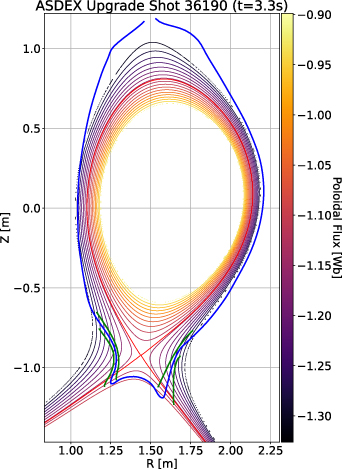
Figure 1. Flux surfaces of the equilibrium used for the simulation. The red line marks the separatrix. The blue line gives the first wall and divertor. The simulation domain extends beyond the divertor legs due to the implementation of parallel boundary conditions via penalisation [33], with the penalisation transition area bounded by the two green lines.
Download figure:
Standard image High-resolution imageOur choice of reference values is guided by parameters and measurements in AUG discharge #36190: major radius R0 = 1.65 m, magnetic field on axis B0 = 2.5 T, density  m−3, electron and ion temperatures
  eV,
eV,  and deuterium ion mass
  . We note that in a global model, reference density and temperature are only required for the normalization of the equations, to write them in dimensionless form as in appendix
  is considered only in the calculation of the electron collision frequency. The resulting dimensionless collisionless parameters of the system – see appendix
  , µ = 2.723 × 10⁻⁴ and ζ = 1. The collisional parameters are
  ,
,  ,
,  ,
,  and
and  . The Braginskii heat conductivity is known to be inappropriate at low collisionality [22, 44, 45]. For instance, it becomes arbitrarily large as ∼T5/2 due to the lack of kinetic flux limiting effects, such as Landau damping. In this work, we use a simple flux limiter which reduces the stiffness and therefore computational expense of the parallel heat conduction:
  . For the chosen reference values, we obtain as reference drift scale and ion Larmor radius
Note that the local Larmor radius varies with magnetic field and temperature. E.g. at reference temperature, it is larger by 25% at the outboard mid-plane due to the reduced local magnetic field of B ≈ 2 T.
In diverted geometry and in absence of neutral gas ionization, we find that density can drop arbitrarily low in the far SOL and private flux region. This contradicts the experimental observation that density can even rise in the far SOL [46], i.e. the simulations are missing the necessary mechanism, e.g. neutral gas ionization. It also makes the solution of the equations unnecessarily expensive, since in particular the parabolic part becomes very stiff at low collisionality. As a simple solution we apply an adaptive source to keep the density above 3 × 10¹⁷ m−3, and temperatures above 3 eV. This source does not hinder cross-field inflow but limits parallel outflow in the far SOL, starting to act above  in the reference simulation, but e.g. only above
  in the simulation in section 5.2. For simplicity, respectively, due to the unphysical core boundary at
  , simulations are adaptively flux driven: the heat and particle sources at the core boundary are adapted in time such as to hold density and temperature fixed there – while in the rest of the domain they evolve freely.
In a global code, background profiles are not chosen but rather evolve freely in accordance with turbulent fluxes. Nonetheless, an initial state must be chosen for the simulation. The most trivial choice would be a flat, or even zero, background profile – which then evolves due to sources at the core boundary. However, in our experience the saturated state is reached faster the closer the initial state is to the final. We choose as initial state for density and temperatures the simple profile as function of 
with

In present simulations, we chose  and
and  . The value
  is held constant between ρ = 0.9 and ρ = 0.92 by an adaptive source. In the SOL, the initial profile is flat and equal to
  .
.
The core boundary, respectively, pedestal top values are chosen in accordance to the experiment as  m−3 and
  eV. The separatrix and SOL initial values are less relevant because they adapt in the course of the simulation. An important restriction comes from the choice of flat SOL profiles: simulations saturate faster with
  as low as possible, since it also initialises lower far SOL values. On the other hand, ideal ballooning stability of the initial profiles prohibits large radial gradients in the confined region, which is correlated with the Greenwald density limit [47]. Our choice for the reference case is
  ,
,  eV and
  eV. In the confined region, electrostatic potential and current are chosen such that the initial pressure profile is stable:
  according to (10), resulting in
  (no vorticity and polarisation velocity), and
  according to (14). The parallel velocity is chosen as zero. In the SOL, the initial state is chosen such that it fulfils the Bohm boundary conditions (A10). Particularly, the parallel velocity is
  at each divertor plate, with a linear dependence on distance between the plates. The initial outboard mid-plane profiles are illustrated in figure 2. To trigger an instability and consequent turbulence, random noise of magnitude 10−5 is added to the density and temperature profiles.
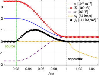
Figure 2. Initial normalized outboard mid-plane (Z = 0) profiles in the reference simulation.
Download figure:
Standard image High-resolution imageFor the reference simulation, we choose as poloidal resolution  mm. Toroidally, we resolve 16 planes. The time step is chosen slightly below the stability limit as
  ns. Due to the limited resolution, the turbulent spectrum must be cut at the poloidal grid scale. To this end, third order hyperviscosity is applied as detailed in appendix
  for all fields. Being able to resolve even smaller scales is highly desirable, particularly in a global code. Eventually, our choice of resolution is a compromise, restricted by the allowable computational expense. Nevertheless, we also performed convergence tests with
  , and a separate test with 24 planes at 2.5ρs0. For the 1.67ρs0 simulation, hyperviscosity was reduced to 300. For the 24 planes simulation, the timestep had to be reduced to 0.7 ns.
It is worth mentioning the computational cost of these simulations, and how it scales. The reference case with 2.5ρs0 poloidal resolution and 16 toroidal planes (∼7 million points) required for simulating 1 ms of the discharge 9 days on 384 processor cores (8 nodes) of the Marconi-A3 SKL partition. As we find saturation only after  ms, at least roughly 0.4 MCPUh and 2 months of patience were required per simulation. Increasing poloidal resolution to 1.67ρs0 raised both the number of grid points and the cost and duration of the simulation by a factor of 2. Increasing toroidal resolution raises the cost quadratically with the number of planes as the maximum allowed timestep is inversly proportional to toroidal resolution, i.e. 24 instead of 16 poloidal planes roughly doubles the cost.
We find no large differences in heat transport with increasing resolution, suggesting that it is mostly captured by the reference case. In detail, however, ion heat transport slightly increases with toroidal resolution, and zonal flows increase with poloidal resolution, as detailed in sections 3.2 and 4, respectively.
3.2. Input power and saturation
In current simulations, fixed density and temperature are prescribed at an artificial core boundary at  – held constant by an adaptive heat and particle source. In figure 3 we show how the input power
  for the reference simulation varies in time – with particle and temperature sources Sn
and
for the reference simulation varies in time – with particle and temperature sources Sn
and  averaged over the whole volume. In the same plot, we show the globally averaged electrostatic potential oscillations (in units of 25 V) – this is due to the GAM, which is always present in global edge simulations [27]. It is important that flux-surface-symmetric potential oscillations like the GAM are permitted up to the core boundary through the implementation of the zonal Neumann boundary condition (see appendix
  saturates at
  ms on a reasonable level: 192 ± 29 kW for electrons and 224 ± 36 kW for ions, with one standard deviation quantifying the oscillations. This is roughly half the input power in AUG discharge #36190.
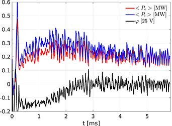
Figure 3. Total electron and ion heating power input in the simulation as a function of time. The globally averaged potential in units of 25 V is also shown. The input power oscillates following the GAM. At later times, it saturates at 196 kW for electrons and 236 kW for ions.
Download figure:
Standard image High-resolution imageIn figure 4, we show zonally averaged separatrix values for density, electron and ion temperatures and electrostatic potential. As indicated by the input power, in the confined region turbulence, and largely also profiles, saturate within 3 ms of simulation time. Further outside, however, time scales are longer due to lower temperatures – particularly in the SOL, where the transit time is of the order 1 ms (as can be estimated from ∼ 50 m connection length and 60 km s−1 flow velocity from figure 5). Turbulence at this time is locally saturated, but globally profiles vary predominantly due to the outflow in the SOL, as we started from flat profiles there. Therefore, for the confined region, the separatrix values are a good criterion for saturation. In the following, we will use the data from  ms for our statistical analysis, although temperatures are still very slowly evolving. Additionally, the globally averaged parallel velocity is shown which is a measure of toroidal rotation. It saturates at 13 km s−1 in the direction of the plasma current – a reasonable value for AUG [49].
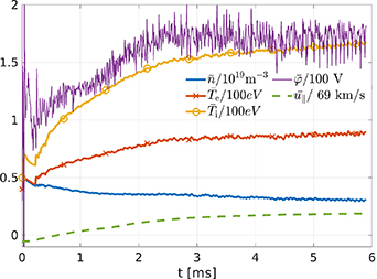
Figure 4. Zonally averaged separatrix density, electron and ion temperatures, and electrostatic potential in normalized units. The parallel velocity shown, averaged over the whole domain, is a measure of toroidal rotation.
Download figure:
Standard image High-resolution image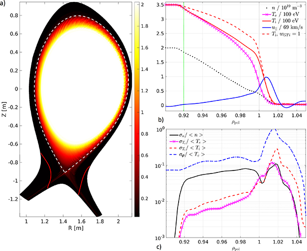
Figure 5. (a) 2D density profile in the poloidal cross section for the quasi-steady state at 7347 µs simulation time for the reference case. The separatrix is shown with a dashed white line, the divertor boundary with a red line. (b) Outboard mid-plane (Z = 0) background profiles, averaged in time over 1 ms and toroidally over 16 planes. 'wGTi
= 1' means with viscous ion heating in the confined region, see also text. (c) OMP fluctuation level, with mean  and variance
  .
.
Download figure:
Standard image High-resolution imageIn unfavourable configuration, i.e. with  away from the X-point, the input power is slightly lower: 187 ± 29 and 204 ± 33 kW for electrons and ions, respectively. The simulation with 24 toroidal planes (higher toroidal resolution) has 176 ± 26 kW for electrons and 221 ± 32 kW for ions, respectively. For the 1.67ρs0 simulation (higher poloidal resolution), we get 187 ± 13 kW for electrons and 221 ± 17 kW for ions – i.e. no significant difference to the reference case with 2.5ρs0. This is remarkable as zonal flows (a radial modulation of the electric field, pressure and parallel velocity) are much more pronounced in the 1.67ρs0 simulation, as discussed in section 4, suggesting that overall thermal transport seems to be barely affected by zonal flows. The reduced oscillation amplitude also indicates a less pronounced GAM. There are no other qualitative differences between the reference simulation and the simulations with higher poloidal or toroidal resolution, as profiles and fluctuation levels remain very similar. Therefore, we conclude that thermal transport is largely resolved in the reference simulation. Increasing resolution further is desirable, but requires a significant speed-up of the code.
3.3. Quasi-steady state profiles, fluctuation levels and transport
Figure 5(a) shows a snapshot of the plasma density in a poloidal plane, in quasi-steady state at  ms for the reference simulation. Figure 5(b) displays profiles at the outboard mid-plane (Z = 0), averaged toroidally and in time over 1 ms, for density, temperature and parallel velocity. While the density profile is rather flat, we see steep pedestals in temperatures around the separatrix – the reason is high heat conductivity, as discussed in section 5.2. Experimentally, pedestals are observed in L-mode at low density, particularly for
  [50].
[50].
We see some penetration of parallel velocity into the confined region, much less than without ion viscosity in figure 11 though. 'wGTi
= 1' stands for active viscous ion heating (in equation (A6)) in the confined region – ions are significantly hotter in that case. It was not possible to run stable simulations with this effect active also in the SOL, hence why the reference simulation is without viscous ion heating – this is further discussed in section 5.1. If active also in the SOL, the heating is even stronger there, leading to non-monotonous  profiles peaking in the SOL and unstable simulations.
Figure 5(c) shows fluctuation levels at the outboard mid-plane. The potential fluctuations are normalised to background (mean) electron temperature, and are the largest in the system. As we have  in the confined region, with
  and
and  fluctuations an order of magnitude smaller, this indicates that turbulence in the confined region is ballooning driven [51, 52]. Around the separatrix, there is a local minimum in
  and
and  , indicating some level of turbulence suppression due to the sheared E × B flow. In the SOL, fluctuation amplitudes peak around
  , at the bottom of the steep gradients. We have here
  , roughly an order of magnitude, but also rather high
  and a steep ion temperature gradient. This suggests a combination of the Kelvin–Helmholtz instability [53, table I] and ITG drive.
The induction of a perturbed magnetic field,  , is crucial for the dynamics of the parallel electric field and current, and therefore electrostatic turbulent transport. The perturbation
  does not necessarily lead to significant additional electromagnetic transport, though: in current simulations, we have
  . In principle, the additional electromagnetic transport can be nonetheless large, depending on the efficiency of parallel (heat) transport along the perturbed magnetic field [54]. However, we have verified that the effect is small in present low-β simulations by additional tests that included electromagnetic flutter (that is therefore otherwise disabled to save a factor 2 in computational time).
Figure 6 shows the difference between one snapshot's density and mean background density – in absolute units of 1019 m−3 (left), as well as normalized to the local mean density (right). Fluctuations are much more prominent on the LFS than on the HFS, which is typical for ballooning modes. In absolute units, fluctuations are negligible in the SOL compared to the confined region – relative to the small local background density, however, SOL fluctuations are much larger, reaching up to 100%, particularly in the region around the X-point where the poloidal magnetic field is weak.
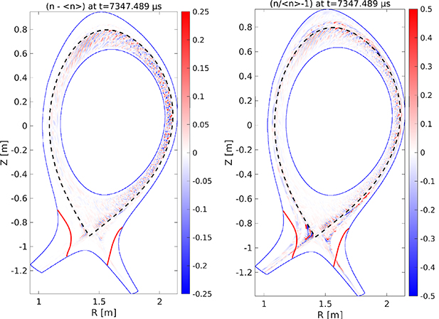
Figure 6. Density fluctuations at a snapshot in quasi-steady state state, at circa 7.3 ms simulation time. Left:  in units of 1019 m−3, right: normalized to the local mean density
  . The separatrix is marked with a dashed black line, the divertor with a red line and poloidal domain boundaries with a blue line. See supplementary movie 2 for the dynamics.
Download figure:
Standard image High-resolution imageWhile figure 6 clearly demonstrates poloidal asymmetries in the transport, we can still compute average radial diffusivities in quasi-steady state. For E × B particle and heat fluxes
we define diffusivities as suggested by [55] via
In the global average  we obtain for the confined region
  m2 s−1,
  m2 s−1 and
  m2 s−1 – reasonable values for AUG experiments [22].
  might imply the presence of the ITG mode – scans of the parallel electron heat conductivity in section 5.2, however, show that this is an effect from diffusive heat flux damping rather than linear instability drive.
  corroborates the finding that turbulence is driven by ballooning modes [55, 56]. Further evidence could be gained by Fourier analysis in field aligned coordinates, particularly from the parallel envelope and the relative phase shifts between the potential, density and temperatures [51, 52] – but this analysis is complicated for us due to the non-field-aligned grid, and will be deferred to future work.
The presented results also hold in the 1.5 times higher resolution simulations (even higher was not yet computationally feasible, as explained in section 3.1). But it should be remarked, as detailed in the next section, that at higher poloidal resolution the increased zonal flow leads to a radial modulation of profiles and fluctuation levels – a staircase structure [57]. However, in present simulations, this has no impact on overall transport (and profiles, disregarding the modulation) as described in section 3.2.
4. The radial electric field
According to our theory developed in section 2, in collisional drift-reduced Braginskii models the equilibrium electric field is determined by the ion particle balance (8) in the confined region and by the sheath boundary conditions (20) in the SOL. We begin by showing in figure 7 the simulated radial electric field in comparison to the ion pressure gradient (and parallel rotation) at the outboard mid-plane (Z = 0) in quasi-steady state. In the SOL, the electrostatic potential follows the electron temperature profile,  , producing a positive electric field. In the confined region, the electric field is negative, which produces counter-propagating flows at the separatrix.

Figure 7. Radial electric field profile vs. ion pressure gradient at the outboard mid-plane, in quasi-stationary phase ( ms), averaged in time over 1 ms and toroidally over 16 planes. The 2.5ρs0 reference simulation is shown on the left and the 1.67ρs0 simulation on the right.
Download figure:
Standard image High-resolution imageThe deviation from  indicates that the equilibrium balance from the diamagnetic compression (9) is accompanied by a contribution from toroidal or turbulence driven zonal flows. In the next section we will show that poloidal rotation is small. If zonal flows are small, too, one can use equation (16),
  , to understand the electric field. In a large aspect ratio tokamak,
  , and so toroidal rotation is mostly given by the parallel velocity. In the left figure 7, in the domain
  , this equality is indeed quite well fulfilled. The deviation, however, is caused by the zonal flow, which becomes even more pronounced with increased poloidal resolution in the right figure.
Zonal flows [5, 48] are typically static in time, but can be overlaid by the GAM oscillation (discussed in section 3.2) and, naturally, turbulent oscillations. They are constant over flux surfaces and have a typical mesoscale radial wavelength [8]. Importantly, we find that high poloidal resolution is necessary to properly resolve the zonal flow production at ρs scale [48, 58] – which is why results throughout this section are compared between the reference simulation at 2.5ρs0 and 1.67ρs0 resolution 6 . On the other hand, equilibrium profiles and input power are nearly identical at both resolutions – see section 3.2. Thus the turbulent transport is barely affected by these zonal flows.
The zonal flow drive is very sensitive to adiabaticity. Only at high adiabaticity the zonal flow drive is efficient [59]. The low wavenumber region responsible for the transport and driving the turbulence is characterized by interchange turbulence, which is less adiabatic. Therefore, this region is less susceptible to the zonal flow. The more drift-wave dominated region around  is responsible for the zonal flow drive, but due to its higher adiabaticity it is not the main driver of the transport. In AUG, low-frequency zonal flows have been not observed so far, not even around the L-H transition [2]. With respect to typical AUG L-mode parameters the present simulations are at particularly low densities and high electron temperatures. Under these conditions the plasma is highly adiabatic, which is beneficial for the generation of zonal flows. However, as we have
  , finite Larmor radius effects should stabilize the region around
  , which in drift-reduced Braginskii models is taken into account only to lowest order. This might lead to an over-prediction of the zonal flow activity.
4.1. Particle, charge and momentum balance on closed field lines
In this section we want to investigate the composition of the mean radial electric field on closed flux surfaces. Zonal flows will be explained by the dominant contributions to the ion particle balance equation (8), averaged in time and over the flux surface. Additionally, the dominant term in the parallel momentum balance – the ion viscous stress (17) – will reveal a non-trivial contribution from the parallel flow. It is important to note that at any single point in time and space, without averaging,  and
and  are by far the dominant terms in the continuity equation (and similarly for
  in the parallel momentum equation), but become less important in a large enough ensemble average, consistent with the neoclassical ordering.
As pointed out in the previous section, the electric field is mostly negative in the confined region, as it mainly follows the ion pressure gradient according to  due to the static equilibrium balance
  (see equation (9)). We are interested in deviations from this balance, and so we show the residue
  by magenta crosses in figure 8. This residue has to be balanced by other terms in the ion particle balance (8). In the flux surface average, parallel derivatives are annihilated, i.e.
  , and the E × B advection
  is mostly small. Therefore, the residue is mostly balanced by the black curve, which is the divergence of the polarisation particle flux
  defined in equation (11). In the average, it is a measure of the Reynolds stress. We therefore conclude that the zonal flow can be understood as the residue between E × B and diamagnetic compression which is sustained by the ion polarisation flux (or equivalently the Reynolds stress),

As explained in the previous section, the zonal flow is driven by near-adiabatic drift waves on Larmor radius scale, and is therefore more pronounced in the higher resolved simulation (but does not necessarily impact overall transport).

Figure 8. Flux surface averaged dominant terms in the ion particle balance equation (black line and magenta crosses) and in the parallel momentum balance equation (red line and blue circles), also averaged in time over 1 ms, in the 2.5ρs0 reference simulation on the left and 1.67ρs0 simulation on the right. Dominant terms in the ion momentum balance are the parts of the stress tensor  , whereby
  .
.
Download figure:
Standard image High-resolution imageThe remaining deviation between the two curves is explained by hyperviscosity  , which is the grid scale numerical dissipation defined in appendix
  is reduced from 3350 to 300 between the 2.5ρs0 and the 1.67ρs0 resolution simulations), it dissipates the energy arriving there due to the turbulent cascade. This process is enhanced by shear layers, and so dissipation is even stronger in the higher resolution simulation. The separatrix deserves particular attention in this regard, since the E × B shear peaks there, as discussed in the next section. Close to to the separatrix, as marked by the yellow ellipse, this results in a peak of
  as well as
  , and also
  largely balanced by
  .
.
It is interesting that the divergence of the polarisation particle flux can in fact be conveniently computed from the quasi-neutrality equation (14). In the flux surface average,  , hence
  . This means that the zonal flow results in
  , i.e. a (predominantly up-down) pressure asymmetry [60]. Additionally, ballooned transport leads to an inboard-outboard asymmetry [60, 61]. Therefore, neither pressure nor the electrostatic potential can be assumed to be constant along a flux surface ψ (thereby
  ).
).
Let us now discuss the role of ion viscosity. Strictly speaking, the Reynolds stress is only contained in the inertial part of the polarisation particle flux  (see section 2.2). However, we find that the viscous part C(G) is always more than two orders of magnitude smaller than the other contributions in the particle balance, i.e. negligible. This means that in present simulations, viscosity does not directly damp the zonal flow. It does, however, efficiently damp poloidal rotation. To see this, we multiply the parallel momentum balance equation (A3) by density n and the magnetic field strength B and average it in time and over flux surfaces. By this, the parallel pressure gradient is annihilated,
  . The remaining dominant contribution is from the viscous stress function G, or more precisely from its constituents. We have defined the ion viscous stress tensor
  in terms of G in section 2.3. We now compare the part of it containing the parallel velocity, plotted in red in figure 8, with the remaining part containing the static equilibrium balance
  , plotted in blue. As the two parts mostly balance, we conclude that poloidal rotation is near zero according to equation (17),

A small deviation is sustained by  and
and  . Importantly, this condition is fulfilled also in spite of pronounced zonal flows in the high resolution simulation – both parts of the viscous stress tensor are modulated, but cancel each other. This means that while viscosity does not directly damp the zonal flow via C(G), it does damp the resulting mean poloidal rotation by adjusting the parallel velocity
  !
!
An important observation is that in the lower resolution simulation (2.5ρs0), the zonal flow is small, but on average over the radial domain constituents of the stress tensor in the parallel momentum balance are the same. In fact, both simulations develop the same mean toroidal rotation (which is roughly the same as parallel rotation in a large aspect ratio tokamak). Although not strictly valid due to the above mentioned necessary asymmetries along a flux surface, equation (16) suggests that parallel velocity also modifies the electric field locally, which seems to be more important than zonal flows in the low resolution case, figure 7 left, at  . The generation, transport and saturation of toroidal rotation are outside the scope of the present study, but a review can be found in [62]. Importantly, in absence of momentum sources in the confined region, as in our present simulations, net toroidal rotation can be only generated in the SOL (see [63]) and transported inward. This is indeed suggested by the parallel velocity profile in figure 5. We point out that ion viscosity seems to be important also for the saturation of this process, as discussed in section 5.1.
The same analysis as above can be performed in a different ensemble average, e.g. toroidal and time (poloidally resolved), as was done in [61] – but more data are required, and results are less concise (2D). A more detailed examination of the generation of mean flows can be found in [41, 64]. We find, consistent with [61], that C(G) is negligible in the vorticity equation. Instead, zonal flows are damped by the GAM oscillation which in turn loses energy through the coupling to Alfvén waves and finally resistivity [48J]. However, we find that this damping is not complete, perhaps because unlike electron pressure, ion pressure does not enter Ohm's law.
4.2. Transition to the SOL: vortex breaking and straining-out at the separatrix
We have shown that the electric field is governed by the ion particle balance in the confined region, and by sheath boundary conditions in the SOL – at least in present simulations. The separatrix has its own specific dynamics as it acts as a boundary between closed and open field lines. We can see this by examining what happens to the turbulent eddies. Figure 9 shows the average shearing rate vs. vortex-turn-over rate at the outboard mid-plane. The former is roughly given by  . The latter is estimated by one standard deviation of vorticity
  , whereby the fluid vorticity is calculated from the generalised vorticity in GRILLIX via
  , with
  .
.
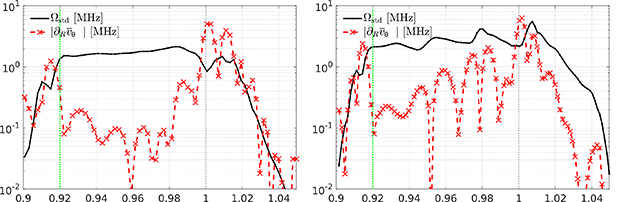
Figure 9. Vortex turn-over rate  compared to the shearing rate ωs
, see text for their definition, in the 2.5ρs0 reference simulation on the left and 1.67ρs0 simulation on the right.
compared to the shearing rate ωs
, see text for their definition, in the 2.5ρs0 reference simulation on the left and 1.67ρs0 simulation on the right.
Download figure:
Standard image High-resolution imageSmall vortices are elongated, thinned and finally absorbed by the shear flow [4, 58, 65] – driving the zonal flow. Stronger vorticies survive. Importantly, as stated in the last section and visible in figure 8, this process extends up to and peaks at the separatrix. Even though larger zonal flows do lead to somewhat higher shearing, we find that the average vortex-turn-over rate is larger than the shearing rate in the confined region at both 2.5ρs0 and 1.67ρs0 resolution – explaining why they have barely any effect on overall transport. At the separatrix additional shearing is provided externally due to sheath boundary conditions and the fast SOL outflow, such that the shearing rate exceeds the vortex-turn-over rate and the eddies can be torn apart. In figure 10, at the top of the device, the tilting of eddies is particularly visible. We highlighted one exemplary vortex breaking event (see [66] for a similar experimental finding). Ultimately, vortices are strained out by the shear flow, and dissipated at grid scale. In the particle balance this manifests as a peaked E × B advection rate balanced by dissipation. Supplementary movie 2 shows the dynamics of density fluctuations.
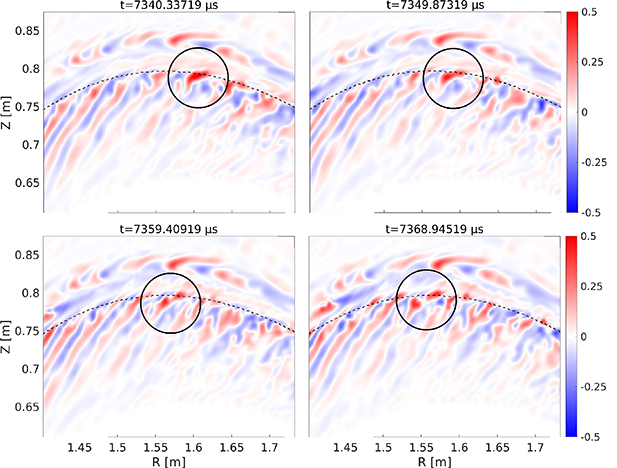
Figure 10. Eddy tilting, straining-out, decorrelation and a single breaking event in the 2.5ρs0 reference simulation, at the separatrix on top of the device (compare with figure 6). Colour scale shows density fluctuation amplitudes relative to the background,  .
.
Download figure:
Standard image High-resolution imageNote also how the far SOL structures appear to be nearly frozen in time in contrast – as temperature in hitting ∼3 eV there, time scales are an order of magnitude slower. These structures, pronounced on the scale relative to the background, are in fact tiny due to the very low background  m−3. Nevertheless, as transport has to saturate globally including the far SOL, its slow dynamics restricts the overall saturation of the simulations.
5. The role of fluid closure terms
Due to the low collisionality in fusion plasmas, the greatest limitation of our model is the collisional fluid closure. In this section we show explicitly its role. This is particularly important as towards lower collisionality, the discussed closure terms – ion viscosity and electron/ion heat conductivity – diverge as ∼T5/2. For the current simulations, a 3D iterative solver [67] allowed us to treat these terms without constraints on the allowed time step – consuming, however, already up to 50% of the computation time. Towards less collisional, hotter regimes (H-mode) additional improvements will be therefore necessary.
5.1. The impact of ion viscosity
The viscosity of ions, represented by the viscous stress function G – see sections 2.2–2.3, is an important dissipation mechanism. In section 4.1 we found that C(G), which enters the perpendicular drifts as a higher order correction, is negligible in the polarisation velocity. On the other hand,  , which enters the parallel momentum balance at leading order, is crucial for damping poloidal rotation. We have also seen in section 3.3 that this damping leads to significant ion heating.
To closer investigate this, we have conducted a simulation without ion viscosity at all (G = 0). The results at t = 2 ms simulation time are shown in figure 11: outboard mid-plane profiles of density, temperature, parallel velocity and electric field. The density profile is very similar to the reference case in figure 5. The electric field is much larger and almost throughout positive, though. The temperature profiles are broader, fluctuations are larger (up to 15% in density in the confined region) and input power is much larger in this simulation – 482 ± 118 kW for electrons and 525 ± 127 kW for ions, respectively – suggesting increased turbulent transport. The larger fluctuation in input power also suggests stronger GAM oscillations.
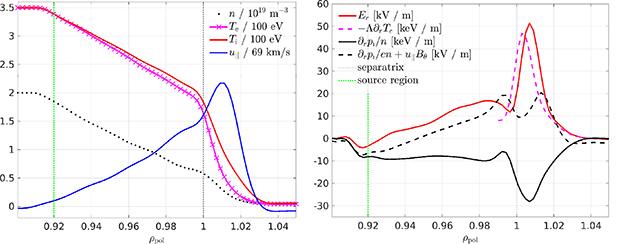
Figure 11. Outboard mid-plane state variables profiles (left) and radial electric field (right) without ion viscosity (G = 0) at t = 2 ms simulation time (saturated turbulence, but flows still evolving). Compare to figures 5(b) and 7 (left).
Download figure:
Standard image High-resolution imageThe electric field is larger in the SOL due to the increased electron temperature gradient. In the confined region, we have performed the same analysis as in section 4.1, finding only a very small contribution from the zonal flow. Although viscosity was disabled in the simulation, we can still compute what the contribution from viscous stress in the parallel momentum balance would have been. Naturally, we find that the viscosity balance (17) is not fulfilled: in the reference simulation, figure 8 left, in an average also over the radial domain, we had  and
and 
 . In the simulation in this section, without viscosity, one would get
 and
and 
 . This means that without viscosity, the plasma obtains a significant poloidal rotation.
At this point, t = 2 ms, the simulation crashes as the electric field starts having large (machine scale) oscillations. A possible reason is the Stringer instability [7, 68], which is expected at low – or absent – viscosity. As the instability is also connected to parallel [60] and toroidal [68] rotation, it is not surprising that we get  . In fact, mean toroidal rotation reaches 26 km s−1 already at t = 2 ms, compared to 13 km s−1 in the saturated reference simulation. However, the inflow of momentum from the SOL [62, 63] and the non-linear Reynolds stress [42] could also be important. At this point, we will not go more into details. But we can conclude that ion viscosity is a crucial mechanism – particularly for damping of poloidal rotation, but also ion heating – and has to be included in realistic tokamak simulations.
5.2. The impact of heat conductivity
The parallel heat conductivity largely determines the parallel heat flux in Braginskii models. Besides obvious consequences for the SOL heat exhaust, circular C-mod simulations [67, 69] have previously shown that flattening of the parallel electron and ion temperature profiles in the confined region can also reduce cross-field transport. To illustrate their impact in current computations, we have repeated the reference simulation with the electron heat conduction lowered to the level of ions, i.e.  instead of 940, and sheath heat transmission factor
  instead of 2.5. The resulting saturated profiles are displayed in figure 12 (unlike with zero ion viscosity, these simulations were running stably).
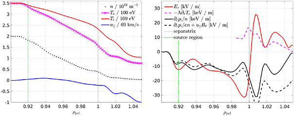
Figure 12. Saturated outboard mid-plane state variables profiles (left) and radial electric field (right) for  and
and  .
.
Download figure:
Standard image High-resolution imageThe most prominent feature is that electron and ion temperature profiles become much broader, including in the SOL, i.e. the pedestal disappears. This is because the profile around the separatrix is determined by the competition of perpendicular transport and parallel outflow, and reducing the heat conductivity and sheath heat transmission significantly hinders the latter. As a secondary effect, due to the increased temperature the ion viscosity increases, damping the parallel flow more strongly. Further, the electric field well deepens. Again, a similar analysis as in section 4.1 reveals that, in this case, this is due to the increased polarisation flux, i.e. zonal flow. This can be either due to a change in the linear instability drive [56], or due to an increased effective resolution: even though the nominal resolution is still 2.5ρs0, the separatrix temperature has increased by roughly a factor 2, such that the effective resolution in terms of the local Larmor radius has increased by  . Similarly as with reduced ion viscosity, the density fluctuation level increases up to ∼15% in the confined region, and input power increases to 535 ± 232 kW for electrons and 463 ± 202 kW for ions, respectively. Noticeably, not only the fluctuations increase, but also electrons are now transporting more heat than ions. This corroborates the hypothesis that transport is driven by ballooning rather than ITG modes, except that for the reference case (with high electron heat conduction) the electron heat flux is more suppressed than the ion heat flux by parallel conductivity.
6. Conclusions
For the first time, global turbulence simulations (using the drift-reduced Braginskii model) have been performed across the edge and SOL of AUG, in diverted geometry and at realistic parameters. Away from the inner boundary of the simulation in the core region of the plasma, the background profiles evolve freely, together with the turbulence. A quasi-steady state is reached asymptotically after about 3–4 ms. The saturated input power of about 400 kW is typical for low density AUG L-mode discharges. At the separatrix, the plasma profiles are determined by a competition between perpendicular transport and parallel outflow. A pedestal develops in the electron temperature due to high parallel heat conductivity.
Particular attention was given to the electric field. On closed flux surfaces, the radial electric field is predominantly determined by equilibrium compression, leading to  . Additionally, we find contributions from toroidal rotation and (in particular) zonal flows. The latter absorb smaller eddies, leading to an inverse energy cascade to larger scales. In the SOL, sheath boundary conditions dominate, forcing the electric field to change sign across the separatrix. The resulting shear flow reinforces straining-out and decorrelation of vortices, leading to intermittent outbursts of up to twice the magnitude compared to the laminar background outflow in the SOL.
The stationary zonal flow, a perturbation between the electric field and pressure with a mesoscale radial wavelength, is driven by the Reynolds stress within the polarisation particle flux. A poloidal resolution scan shows that the drive happens on Larmor radius scale by near-adiabatic drift waves which do not significantly contribute to transport. On the other hand, fluctuation levels and average diffusivities suggest that transport is driven by larger scale interchange modes, i.e. coarse simulations are able to mostly capture the transport.
The role of the fluid closure terms – ion viscosity and heat conductivities – was explicitly examined. We find that ion viscosity is negligible in damping vorticity, but highly effective in damping poloidal rotation by adjusting of the parallel velocity profile, while also generating considerable ion heating through magnetic pumping. The electron and ion heat conductivities, on the other hand, are important for parallel heat fluxes, and they largely determine the pedestal and SOL temperature profiles. Both damping mechanisms, viscosity and heat conduction, affect the electric field and reduce the perpendicular transport.
A limiting factor for the simulations is their computational cost. MPI communication and OpenMP performance are currently being optimized, which should allow for faster medium-sized tokamak simulations, also including magnetic flutter (important at higher beta [70]). For larger devices like ITER and DEMO, a larger speed-up or scalability is required, by means of GPU accelaration or 3D MPI domain decomposition.
Further work is needed to extend the applicability of our model to H-mode conditions. Most pressing, as the Braginskii fluid closure loses validity towards lower collisionality regimes, Knudsen corrections [71] (modelling Landau damping [72]) will have to be introduced for heat conductivities. The ion viscosity will have to be adapted to properly model the neoclassical electric field [22, 73]. In this regard, generation and damping of poloidal and toroidal rotation should be studied in more detail. Ways to include the ion orbit loss effect [74, 75] should be explored, as this might explain why so far we found no significant difference between the favourable and unfavourable direction of the toroidal magnetic field. Furthermore, even in attached L-mode regimes, the applicability of our model in the SOL is yet limited. In our current simulations, the SOL electric field is determined by an isolating sheath, and the pressure profile by the competition between turbulent cross-field transport and parallel outflow. In a real SOL, the sheath can conduct significant currents, and neutral gas recycling and impurities lead to complex density and temperature profiles and flows. The resulting strong gradients between the outboard mid-plane and the divertor, and particularly plasma detachment, are of great interest for fusion reactors. Correspondingly, the incorporation of the aforementioned effects is being urgently pursued.
Acknowledgments
The authors thank E Wolfrum, A Bergmann, E Poli, M Francisquez, B N Rogers, E Fable, T Görler, A Chankin, J Loizu, V Rozhansky, A Cathey Cevallos, M Faitsch, R W Brzozowski III and S Makarov for helpful discussions. This work has been carried out within the framework of the EUROfusion Consortium and has received funding from the Euratom research and training programme 2014–2018 and 2019–2020 under Grant Agreement No. 633053. The views and opinions expressed herein do not necessarily reflect those of the European Commission. B Zhu is supported by the U.S. Department of Energy Contract DE-AC52-07NA27344 through the Lawrence Livermore National Laboratory.
Appendix A.: Global drift-reduced Braginskii equations in GRILLIX
The current physical model in GRILLIX builds on its recent extension by hot ions [67]. The most important newly added terms arise from the ion stress tensor [36], particularly its viscous part. Additionally, collisional electron-ion heat exchange was added.
In the following, time scales are normalised to  , with R0 the major radius and
  the sound speed at reference electron temperature
  . Perpendicular scales are normalised to the sound Larmor radius
  (in CGS units) and parallel scales to R0. The dynamical fields evolved in GRILLIX are the density n normalised to a reference density n0, the electrostatic potential ϕ normalised to
  , the parallel ion velocity
  normalised to cs0, the electron and ion temperatures
  and
and  normalised to reference values
  , respectively,
  , the parallel current
  normalised to
  and the parallel component of the perturbed electromagnetic potential
  normalised to
  with
with  .
.
The normalized equations (A1)–(A7) represent electron continuity equation, vorticity equation, parallel momentum balance, Ohm's law, electron and ion temperature equations and Ampere's law. The advective derivative is defined as  and the curvature operator as
  . The equation set requires a number of auxiliary quantities: The parallel electron velocity
  , the electron and ion pressures
  , respectively,
  , generalized vorticity
 ![$\Omega = \nabla\cdot\ \left[ \frac{n}{B^2}\left(\nabla_\perp\varphi+\zeta \frac{\nabla_\perp p_\mathrm{i}}{n}\right)\right]$](https://content.cld.iop.org/journals/0741-3335/63/3/034001/revision4/ppcfabd97eieqn204.gif) and generalised electromagnetic potential
and generalised electromagnetic potential  . The ion viscous stress function G was defined in equation (13) and is normalized as
  . The parallel gradient is defined as
  , with
  the unit vector of the background magnetic field. While electromagnetic induction is taken into account in equation (A4), transport by electromagnetic fluctuations (flutter) is implemented, but currently disabled due to significant additional computational cost.
The four dimensionless, collisionless parameters of the system are the drift scale  , dynamical plasma beta β0 defined above, and electron to ion mass and temperature ratios
  , respectively,
  . For the collisional parameters, we require
  and
and  – the electron, respectively, ion collision times evaluated at reference temperature and density and normalised to
  . Then, the remaining five dimensionless collisional parameters of the system are the electron collisionality
  , normalised parallel resistivity
  , normalised parallel electron and ion heat conductivities
  , respectively,
  , and normalized ion viscosity
  . Additionally, via the parameter wGTi
, ion viscous heating which is usually dropped in literature [36] can be switched on and off.
. Additionally, via the parameter wGTi
, ion viscous heating which is usually dropped in literature [36] can be switched on and off.


Sn
,  and
and  are source functions driving the system with particles and energy. For numerical reasons, respectively, in order to cut the turbulent spectrum, a dissipation is added to all equations of the form

with constants  ,
,  for every field.
  is zero in most of the domain, but is high in the last few grid points towards the radial boundaries. For hyperviscosity, N = 3 is chosen.
The system is energy conserving, with the exception of numerical dissipation, neglect of polarisation velocity in perpendicular advection and boundary conditions. We note that parallel viscosity in equation (A3) is treated implicitly, similarly to electron and ion heat conduction [67], while all other terms are advanced explicitly in time.
At the inner and outer limiting flux surfaces, the following homogeneous boundary conditions are applied

to prevent particles and energy fluxes through the boundary. For the potential, the sheath boundary condition  is applied at the outer wall boundary. At the inner (core) boundary
  , the zonal homogeneous Neumann boundary condition
  and
and  is applied, which allows the potential to float but prevents net E × B flux through that boundary.
At the divertor, insulating Bohm sheath boundary conditions are applied

where Λ = 2.69 and  .
.
For further numerical details on the implementation of the model in GRILLIX, e.g. the FCI approach and the immersed boundary technique, we refer to previous publications [33, 67, 76, 77].
Footnotes
- 4
- 5
One difference between experiment and simulation is the choice of the helicity of the poloidal magnetic field: in the experiment, the plasma current flows in the opposite direction to the toroidal magnetic field, while we chose them to be parallel in most of our simulations, i.e. the poloidal magnetic field rotates in the opposite direction. However, we have repeated the reference simulation (defined below) with the correct helicity and found no physical difference except the direction of toroidal rotation – within a poloidal plane, nothing changes at all.
- 6
Note that in a global computation the local Larmor radius ρs changes strongly throughout the domain – refer to section 3.1 for a detailed description of the simulation setup for both cases.
