
Abstract
In this study, enhanced radial transport in a volume-recombining region in detached helium plasmas in a linear device, Magnum-PSI, was investigated. By installing a reciprocating Langmuir probe, electrostatic fluctuations with high spatiotemporal resolutions were measured and analyzed. As a result, the ion-flux profile broadening in the detached state and the coherent plasma structure, which has an internal electric field in the azimuthal direction, were confirmed. By analyzing the emission intensities obtained with a fast framing camera viewing around the probe head, an enhanced fluctuation, which has an azimuthal mode number of m = 1, was found to be correlated with radial plasma ejection. This m = 1 mode rotates by the drift with the radial electric field and magnetic field and is correlated with the m = 0 mode. These two modes behave like a predator and prey; they quasi-periodically appear with about a quarter-period shift. Because the ion flux flowing into the target plate decreases when the radial transport is enhanced, this cross-field transport disperses the ion flux and decreases the maximum heat load applied to the target.
Export citation and abstract BibTeX RIS

Original content from this work may be used under the terms of the Creative Commons Attribution 4.0 license. Any further distribution of this work must maintain attribution to the author(s) and the title of the work, journal citation and DOI.
1. Introduction
Plasma detachment is essential for reducing the heat flux to the divertor target. Recent experiments have suggested that the detached plasma enhances the nondiffusive cross-field transport in the edge regions of several magnetic configuration devices, including tokamaks, heliotrons, and linear devices [1–9]. Such enhanced transport broadens the divertor heat load across the magnetic field, and consequently, the maximum heat load can be less than that when the transport is not enhanced. Furthermore, cross-field transport can affect the detached plasma formation and its stability [9]. To improve the prediction accuracy of the divertor heat load for future fusion devices, it is necessary to clarify the enhancing mechanism of radial plasma transport and its parameter dependence, including the ITER divertor condition.
Although a linear configuration has massive advantages in terms of flexibility, steady-state nature, and reproducibility to reveal detailed transport characteristics, it exhibits much lower plasma density and magnetic field strength than the ITER divertor condition in almost all devices globally. However, the linear plasma device MAgnetized plasma Generator and NUMerical modeling for Plasma Surface Interactions (Magnum-PSI) at DIFFER, which has started operation with a superconducting coil since 2017, can realize ITER-relevant-density plasma production at a high magnetic field strength [10–12]. Comparisons between Magnum-PSI and other devices can be used to forecast the transport characteristics in ITER and DEMO divertor plasmas. However, because of the extremely strong heat flux in Magnum-PSI, a Langmuir probe, which is useful for measuring plasma transport with high spatiotemporal resolution, is not equipped as a permanent measurement device, and thus, satisfactory fluctuation studies have not yet been conducted.
This study performed electrostatic fluctuation measurements and analyses by installing a reciprocating Langmuir probe in Magnum-PSI. To reduce the heat load on the probe head, a magnetic field condition (B = 0.4 T) lower than that in a typical operation was employed as an initial step toward more ITER-relevant conditions. In addition, a fast framing camera was used to capture a wide spatial range around the probe head, and the target-plate ion current was simultaneously acquired with a high temporal resolution.
Previous studies conducted on a linear divertor plasma simulator, NAGDIS-II, have found that the cross-field transport is enhanced in an axially localized region where the volume recombination strongly occurs in pure helium (He) plasmas [7–9]. Because no molecular-relevant recombination processes occur in pure He plasmas, the volume-recombining region is more localized in He plasmas than in hydrogen isotope plasmas. In this study, to investigate the relationship between a volume-recombination region and transport characteristics in Magnum-PSI, pure He plasmas were produced with different gas flow rate scanning from attached to detached divertor plasma condition. By applying several statistical analysis techniques, the spatiotemporal behavior of the cross-field transport was revealed and compared with that of NAGDIS-II.
In the following section, the experimental setup of the fluctuation-measurement devices is explained. In section 3, the neutral pressure dependences of the measured signals are shown. Detailed fluctuation characteristics and spatiotemporal behaviors are investigated in sections 4 and 5, respectively. This study is summarized and some of the obtained results are discussed in section 6.
2. Experimental setup
Magnum-PSI is a unique linear superconducting device that can realize ITER-relevant divertor plasmas with high ion fluxes of up to 1025 m−2s−1 under strong magnetic field conditions [10, 12]. Plasmas are generated by a DC-cascaded arc discharge; typical plasma parameters include an electron density of ne ∼ 1020–1021 m−3 and an electron temperature of Te ∼ 1–5 eV; the magnetic field can reach B = 2.5 T [12]. A differential pumping system comprising two orifice plates (skimmers) and roots pumps divides the vacuum vessel into three parts. This configuration enables a detailed comparison between the attached and detached states in the downstream part of the vacuum vessel, which is called the 'target chamber,' under similar source plasma conditions. In the target chamber, a highly accurate Thomson scattering (TS) system, with a small error even in the detached plasmas, is operated to obtain ne and Te profiles along the radius (rTS) in front of the target [13, 14]. The same axial position (hereafter 'TS axial position') is also observed using a single-position passive spectroscopy system (Avantes AvaSpec-2048-USM2-RM), which views radially through the plasma to acquire survey line-integrated emissions from the plasma over the range of 299–950 nm [12].
This study mainly analyzed the fluctuation signals obtained at the TS axial position, as shown in figure 1(a). To measure high-spatiotemporal-resolution signals, a Langmuir probe system mounted on a reciprocating arm was installed. Additionally, a fast framing camera viewing a wider area around the probe head was used. Furthermore, the total ion flux flowing into the target plate was measured. The detailed setup of these fluctuation measurements is described below.
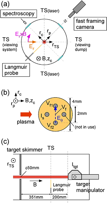
Figure 1. Schematics of (a) the measurement system at the TS axial position, (b) Langmuir probe head, and (c) side view of the vacuum vessel.
Download figure:
Standard image High-resolution image2.1. Langmuir probe
In this study, a reciprocating Langmuir probe was installed at the TS axial position. The reciprocation system was the same as that used in previous studies conducted on Pilot-PSI [15] and Magnum-PSI [16]. In a previous experiment conducted on Magnum-PSI [16], an ion-sensitive probe measurement was performed.
Figure 1(b) shows a schematic of the newly applied probe head with multiple electrodes. This probe head was formed of a 4 mm-diameter ceramic shaft and four 0.5 mm-diameter tungsten electrodes with an exposed length of 0.5 mm. Three of these electrodes were used for measuring the ion saturation current (Is) and two floating potentials (Vf1, Vf2). The probe electrode for Is was positioned at the upstream side and biased at −100 V. The other two electrodes for Vf1 and Vf2 were positioned perpendicularly to the magnetic field at a distance of d = 2 mm to measure the azimuthal electric field (Eθ), as described later. The floating potential at the midpoint connected to the Is-measuring electrode along the magnetic field was deduced by Vf = (Vf1 + Vf2)/2. These signals were simultaneously acquired at a sampling frequency of 500 kHz by using isolated analog-to-digital converters (Yokogawa 720254, 16 bits).
During discharge, the probe head was moved from a radius of rp = −50 mm to the radial center (rp = 0) through compressed air (figure 1(a)). After a few seconds of measurement at rp = 0, the probe head was extracted to minimize the damage caused to the probe materials by the steady-state plasma. The probe position was measured with a mark sensor by reading a barcode every 1 mm. The insertion and extraction speeds were ∼200–300 mm s−1. This study only analyzed insertion and stationary phases (i.e. data during probe withdrawal were not included).
As shown in figure 1(c), at 351 mm upstream of the TS axial position, there was an electrically floating orifice plate, called the 'target skimmer.' Because the inner diameter of the target skimmer was 50 mm, the peripheral region at |rp| > ∼25 mm at the TS axial position was not connected to the plasma source along the magnetic field.
2.2. Fast framing camera
A fast framing camera (Phantom V12, 12-bit grayscale) was used to capture a wide spatial region around the probe head. From the window opposite to the port where the probe system was mounted (figure 1(a)), a line-integrated visible light emission (Iem) perpendicular to the magnetic field was obtained without any optical filter. As shown in figure 1(a), rc is defined as the distance from the plasma center in the direction perpendicular to the line of sight and magnetic field. In addition, zc represents the axial displacement from the TS axial position along the magnetic field direction. The frame rate and exposure time were set to 97 073 fps and 3 μs, respectively, and the frame size and pixel resolution were 128 × 256 and ∼0.36 mm pixel−1.
Figure 2 shows typical profiles of the mean values of Iem over a steady-state time period,  , in the recombination front, where
  indicates the average. The circular low-μem regions observed at the edge are outside the window outline. In figure 2(a), the probe head is fixed at the far periphery (rp = −50 mm) and μem slightly decreases along the magnetic field with zc increasing from upstream to downstream. In contrast, with the probe insertion (rp = 0) in figure 2(b), the μem amplitude rapidly decreases at zc ∼ 0 and downstream of this position. Because there is a plasma flow from the upstream, the disturbance to the plasma on the downstream side is strong. Additionally, because the probe diameter is not significantly smaller than the plasma-column diameter, the presence of the probe shaft creates a certain energy sink. Thus, the emission intensity in the upstream region is also slightly weakened. Furthermore, a local minimum of μem is found at (rc, zc) ∼ (−3, 0) mm in figure 2(b), which indicates the exact probe position when rp = 0. Therefore, the most inward position of the Langmuir probe head is ∼3 mm distant from the plasma center in the negative rc direction.

Figure 2. Profiles of μem in the recombination front (P = 2.2 Pa), where the probe positions are (a) rp = −50 and (b) 0 mm. (c) The profile of μem under the lowest neutral pressure condition (P = 0.44 Pa).
Download figure:
Standard image High-resolution imageFigure 2(c) shows μem under the lowest neutral pressure condition used in this study. The emission intensity is the background level, and we cannot analyze the Iem fluctuation in this case. As described later, because the electron temperature monotonically decreases with an increase in the neutral gas pressure, the emission intensity attributed to the ionization process is maximum under this low-pressure condition, despite the background-level emission. Therefore, most of the emission from recombining plasmas is attributed to the excited neutrals generated through the volume-recombination processes.
2.3. Target plate
Magnum-PSI has a long target manipulator system, which can install various target shapes [17]. In this study, the target plate facing the main plasma was positioned 200 mm behind the TS axial position, as shown in figure 1(c). The shape of the target structure was not simple; it had five small target holders, whose detailed design is shown in [17]. The target was composed of a molybdenum sample mounted with a 64-mm-diameter hollow tantalum holder on a metal structure, which had a square surface with a side length of ∼64 mm. Considering the magnetic field geometry and spatial relationship, the measuring range of |rp| < ∼45 mm at the TS axial position would connect to the target plate along the magnetic field, while the far periphery at |rp| ∼50 mm would not connect to the target. In this study, the target plate was biased negatively at ∼−60 V and the total ion saturation current (Itgt) over the target was measured using a current probe.
3. Neutral pressure dependence of measured signals
This study investigated pure He plasmas with B = 0.4 T. The discharge current was set to 120 A and the discharge voltage was almost constant at 75–78 V. He gas was introduced with a flow rate of 15 slm into the source region, which corresponds to the maximum operational limit. A gas feed allowed the injection of gases into the target chamber. The gas flow into the target chamber was varied from 0 to 6.9 slm to change the downstream plasma condition from ionizing (attached) to recombining (detached) state. At that time, the neutral gas pressure in the target chamber (P) was ∼0.44, 1.4, 1.8, 2.2, 3.0, 3.9, 4.7, 5.6, and 6.4 Pa.
This section shows the neutral pressure dependences of the signals measured using the spectroscopy, TS, and Langmuir probe systems.
3.1. Line-emission intensities and plasma parameters
Figure 3(a) shows the neutral pressure dependences of line-emission intensities from highly excited states (He I: 23P–73D, 23P–83D, 23P–93D, 23P–103D, wavelength: 370.5, 363.4, 358.7, and 355.4 nm, respectively) at the TS axial position. Here, the line emissions are observed to be quite small in the lowest pressure case of P = 0.44 Pa, while they are high at P ∼ 1.8–3.9 Pa. At P = 4.7 Pa or more, the intensity decreases with increasing P. Therefore, recombining plasmas were generated except for that in the P = 0.44 Pa case. The recombination front, which is defined as the region where the electron-ion volume recombination strongly occurs [8, 9], exists near the TS axial position at P ∼ [2, 4] Pa and moves upstream at P > ∼4 Pa.
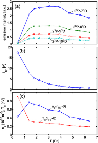
Figure 3. Neutral pressure dependences of (a) line-emission intensities at 23P–73D (solid), 23P–83D (dashed), 23P–93D (dotted), and 23P–103D (dashed dotted); (b) Itgt; and (c) ne (solid) and Te (dashed) around the plasma center.
Download figure:
Standard image High-resolution imageSimilarly, the Itgt dependence on P is plotted in figure 3(b). By increasing P, Itgt monotonically and rapidly decreases due to the plasma detachment. At P = 6.4 Pa, Itgt becomes 25 times smaller than that at P = 0.44 Pa.
Figure 3(c) shows the ne and Te dependences on P measured with TS, which are averaged values around the plasma center (rTS = [−2, 2] mm). Due to the small B, ne is smaller than its typical range of Magnum-PSI. By increasing P, ne increases from ∼4.3 × 10¹⁹ m−3 at P = 0.44 Pa to ∼7.7 × 10¹⁹ m−3 at P = 1.4 Pa, and then monotonically decreases, showing a rollover. In contrast, Te suddenly decreases from ∼0.90 eV at P = 0.44 Pa to ∼0.34 eV at P = 1.4 Pa. Then, Te monotonically decreases with increasing P and reaches ∼0.19 eV at P = 6.4 Pa.
Figure 4 shows the radial profiles of ne and Te measured with TS at P = 0.44, 1.4, 2.2, and 6.4 Pa. Most of the TS measurement range is within the target skimmer radius at |rTS| ∼25 mm. Each profile has an axisymmetric profile, and the full width half maximum of each ne profile is larger than 20 mm, which is larger than the typical width in Magnum-PSI because of the weak magnetic field [12]. At P = 0.44 Pa, ne has a flat profile around the radial center, while Te has a hollow profile at |rTS| < ∼15 mm. In contrast, at higher P cases, ne has Gaussian-like profiles and Te values are flatter. Because Te ≪ 1 eV except for P = 0.44 Pa, the electron-ion recombination process dominantly occurs, which reduces the plasma density and ion particle flux flowing into the target.

Figure 4. Radial profiles of (a) ne and (b) Te at P = 0.44 (solid), 1.4 (dashed), 2.2 (dotted), and 6.4 Pa (dashed dotted).
Download figure:
Standard image High-resolution image3.2. Electrostatic-signal statistics
To determine the neutral-pressure dependence of Is measured with the Langmuir probe, its radial profile is contour-plotted along P, as shown in figure 5(a). Here, linear interpolation is performed between the discrete data points along P. The ion saturation current, which is proportional to the ion flux, is concentrated inside the target skimmer radius and decreases with increasing P at |rp| < ∼25 mm. In contrast, focusing on the peripheral region behind the target skimmer, an increase and then a decrease in Is with increasing P are observed with a peak at ∼2.5 Pa. As a result, the radial profile of Is becomes broader (flatter) toward the periphery at P ∼ 2.5 Pa. This broadened profile is observed in the recombination front with high line-emission intensities (figure 3(a)), which is similar to the previous studies conducted on NAGDIS-II [7, 8]. Interestingly, the Is radial profiles at P ∼ 1.4 and 1.8 Pa have a clear dip along rp with a minimum at around |rp| ∼ 35–40 mm.
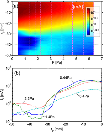
Figure 5. (a) Neutral pressure dependence of the radial profile of Is. Vertical dashed lines indicate P values where the Langmuir probe measurements are performed. (b) Logarithmic plot of Is as a function of rp at P = 0.44 (solid), 1.4 (dashed), 2.2 (dotted), and 6.4 Pa (dashed dotted).
Download figure:
Standard image High-resolution imageFigure 5(b) shows the logarithmic plot of the radial profiles of Is at P = 0.44, 1.4, 2.2, and 6.4 Pa. Note that there would be some plasma disturbance at rp ∼ 0, besides the fact that the rp = 0 position is a few millimeters distant from the accurate plasma center, as mentioned in section 2.2. Therefore, the Is peak observed at rp < 0 in each case is attributable to the ion-flux reduction inside the plasma column by probe insertion. At P = 0.44 Pa, log10(Is) has a steep gradient at rp ∼ −27 mm and is quite small in the periphery. At P = 1.4 Pa, the steep-gradient position shifts radially outward by ∼5 mm. Furthermore, Is increases at rp < ∼ −42 mm compared to the P = 0.44 Pa case. As a result, a dip with a small Is is observed at rp ∼ [−40, −32] mm. At P = 2.2 Pa, this dip disappears by further profile broadening. Under higher pressure conditions of P > 2.2 Pa, Is decreases in the radial range.
Figure 6 shows the Vf profiles (a) as functions of rp and P and (b) as a function of rp at P = 0.44, 1.4, 2.2, and 6.4 Pa, where radially hollow profiles around the radial center can be observed. By using Vf and Te, the plasma potential (Vp) can be calculated as Vp ∼ Vf + 3.7Te under the assumption of Te = Ti [8, 9], where Ti is the ion temperature. Figure 6(b) shows the radial profiles of Vp calculated with Vf and Te, which are obtained by Langmuir probe and TS measurements, respectively. Here, Te at rp is assumed to be equal to that at rTS. The Vp profiles are qualitatively similar to the Vf profiles, but higher due to the Te component. Except for the lowest neutral pressure case, the Te values are much lower than 1 eV (figure 4(b)). As a result, the Vp profiles are similar to the Vf profiles shifted up by ∼1 V in recombining plasma cases.
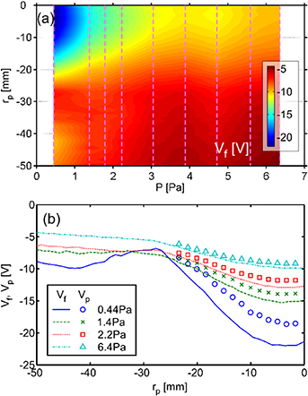
Figure 6. (a) Neutral pressure dependence of the radial profile of Vf. Vertical dashed lines indicate P values where the Langmuir probe measurements are performed. (b) Radial profiles of Vf (lines) and Vp (markers) at P = 0.44 (solid/circle), 1.4 (dashed/cross), 2.2 (dotted/square), and 6.4 Pa (dashed dotted/triangle).
Download figure:
Standard image High-resolution imageThe negatively biased cathode in the cascaded arc discharge makes the Vp radial profile of hollow shape, particularly in the ionizing plasma at P = 0.44 Pa. By promoting plasma detachment by increasing P, the Vp profile becomes shallower, which is similar to the axial Vp change in NAGDIS-II [8, 9, 18].
4. Detailed fluctuation characteristics
In section 3, it was found that the ion-flux profile broadening appeared in the recombination front. In this section, detailed fluctuation characteristics are investigated.
4.1. Frequency characteristics
Figure 7 shows the power spectra of Is as functions of frequency (f) and rp at P = 0.44, 1.4, 2.2, and 6.4 Pa. In the ionizing plasma at P = 0.44 Pa, a large spectral peak is observed at f ∼ 30 kHz around rp = [−18, −4] mm. By increasing P, this high-frequency component appears to weaken and shift to the low-frequency side. Furthermore, an additional frequency peak is observed around f = 6 kHz at the outer radial position in recombining plasmas (P ≥ 1.4 Pa). In the recombination front at P = 2.2 Pa, this component exists around rp = [−25, −10] mm. Its peak frequency slightly increases with decreasing |rp| within the range of f ∼ [3.5, 10] kHz, and apparently connects to the higher-frequency component at f > ∼10 kHz in the radially inner region. Moreover, strong f < ∼3.5 kHz components are confirmed around the radial center and in the periphery (|rp| > ∼30 mm). Regarding the low-frequency component in the periphery, the appearing radial range in each P case simply corresponds to the region where the Is value is high, as shown in figure 5.
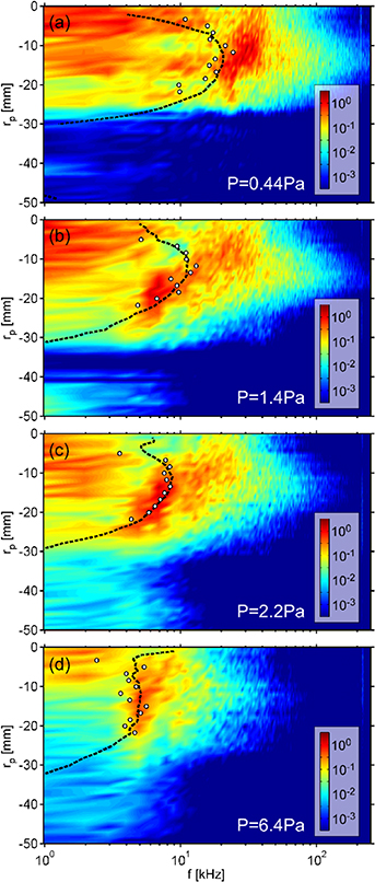
Figure 7. Contour plots of power spectra of Is as functions of f and rp at (a) P = 0.44, (b) 1.4, (c) 2.2, and (d) 6.4 Pa. Black dashed lines and circles indicate the estimated fθ obtained from Vf and Vp, respectively, along rp.
Download figure:
Standard image High-resolution imageBelow this subsection, detailed frequency characteristics at P = 2.2 Pa will be focused.
Figure 8(a) shows the power spectra of Is at rp = 0 and −50 mm, which correspond to the innermost and outermost positions, respectively, with a higher frequency resolution than that shown in figure 7(c). Additionally, the power spectra of Vf at rp = 0 and −50 mm and Itgt are plotted in figure 8(b). At f = 20, 40, 80, ... kHz, several sharp peaks are clearly observed for Itgt, which are likely attributed to the discharge-power-supply noise in Magnum-PSI. These noise components with the same frequencies are also observed for Is, particularly at rp = −50 mm, but are not as outstanding as Itgt. Furthermore, there is a strong peak at f ∼ 220 kHz, particularly in the power spectra of Vf, which may be due to some phenomenon because its amplitude becomes high inside the plasma; however, this fluctuation is beyond the scope of this paper. The power spectrum of Is at rp = −50 mm has a flat and inclined slope with a shoulder at f ∼ 4.5 kHz. Such a shoulder in the power spectrum is widely observed in the edge plasmas of several devices [19] when coherent structures such as blobs nonperiodically appear in a time series [20]. At rp = 0, a shoulder or a little convex is observed at f ∼ 1.5 kHz. Furthermore, a small maximum is observed at f ∼ 20 kHz. The latter is connected to the high-frequency component observed in figure 7(c). In contrast, the power spectrum of Itgt has a little convex at f ∼ 1.5 kHz, which is the same with the shoulder frequency of Is at rp = 0.

Figure 8. Power spectra of (a) Is at rp = 0 (solid) and −50 mm (dashed), Iem at rc = 0 (dotted) with probe insertion (rp = 0), (b) Vf at rp = 0 (solid) and −50 mm (dashed), and Itgt (dotted). Note that 1/100 times value is plotted as the Iem power spectrum in (a).
Download figure:
Standard image High-resolution imageAlthough the Langmuir probe is beneficial for measuring the local fluctuations, it might disturb the fluctuation characteristics, such as amplitude and frequency. To clarify the probe insertion effects on the fluctuation, Iem signals obtained by the fast framing camera were investigated. Because the probe structure is included in the line of sight at the exact TS axial position (figure 2(b)), the fluctuation characteristics of Iem in the vertically elongated rectangular pixels at zc = −10 mm are investigated below.
Figure 9 shows the power spectra of Iem as functions of f and rc without probe insertion (rp = −50 mm) and with probe insertion (rp = 0) at P = 2.2 Pa. It is confirmed that typical peak frequencies and spectral shapes are almost the same irrespective of whether or not the probe is inserted, although the fluctuation amplitude becomes weaker due to the probe insertion. The profile of the Iem power spectra resembles that of Is in figure 7(c). The Iem power spectra at rc = 0 with probe insertion is superimposed in figure 8(a). The spectral peaks of Iem at f ∼ [3.5, 10] kHz, which connect to the higher-frequency region, have no strong amplitude at rc = 0 in figure 9. The small 20-kHz maximum observed in the Is power spectrum at rp = 0 is attributable to the slight deviation of the probe head from the radial center, as mentioned in section 2.2. In contrast, the low-frequency component at f < ∼3.5 kHz is strong at the radial center in both Iem and Is power spectra. The same frequency component is also strong around |rc| = 22 mm.
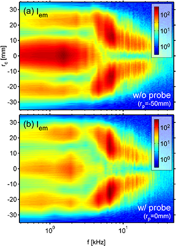
Figure 9. Contour plots of power spectra of Iem at zc = −10 mm as functions of f and rc at P = 2.2 Pa, where (a) rp = −50 mm and (b) 0 mm.
Download figure:
Standard image High-resolution imageOwing to the line-integral effect, odd and even modes along the azimuthal direction should become weak and strong, respectively, at rc = 0 [21]. Therefore, strong fluctuation components at f> ∼3.5 kHz and f < ∼3.5 kHz have odd and even azimuthal mode numbers (m), respectively. The low-frequency component at the radial center has a small maximum at f ∼ 1.5 kHz. If this component is attributed to an even mode rotation with m = 2 or more, this rotation should occur at a radius of ∼22 mm or more, considering the line-integral effect [21]. Furthermore, the total ion flux flowing into the target plate, which covers a radius of 32 mm, is not sensitive to the rotation phenomenon (m ≥ 1) within its radius, owing to the integration effect in the azimuthal direction. However, as shown in figure 8, similar maxima at f ∼ 1.5 kHz are confirmed in the power spectra of the local fluctuation of Is at rp = 0 and Itgt. Therefore, the mode number of the low-frequency component can be designated as m = 0.
4.2. Azimuthal rotation with Er × B drift
By using the Vf and Vp radial profiles in figure 6, the Er × B rotation frequency (fθ) can be estimated, where Er is the radial electric field. Because Er = −dVp/drp, the azimuthal rotation speed (vθ) can be calculated by the Vp radial profile as vθ = Er/B = (−dVp/drp)/B. Furthermore, if the contribution from the Te gradient is negligible, vθ ∼ (−dVf/drp)/B. By using vθ, fθ = vθ/2πrp can be obtained as a function of rp. Owing to the hollow potential profile, the Er × B direction corresponds to the clockwise direction viewed from the source region, as shown in figure 1(a).
The estimated fθ profiles from Vf and Vp are superimposed with black dashed lines and circles, respectively, in figure 7. Because of some disturbance and an inaccurate radial position, the estimated fθ near the plasma center is not reliable. The fθ values calculated from Vf and Vp are almost similar in all P cases. Therefore, the contribution of the Te gradient is much smaller. At P = 0.44 Pa, fθ is smaller than the spectral peak frequency of f ∼ 30 kHz around rp = [−18, 4] mm. In contrast, fθ shows good agreement with the spectral peak around f = 6 kHz at rp ∼ [−25, −10] mm in the recombining states. A mode rotation with rotation frequency fθ generates a fluctuation with the frequency of mfθ at any fixed position. Therefore, this frequency match indicates that the mode number of the periodic fluctuation at f ∼ 6 kHz is m = 1.
4.3. Cross-correlation between Is and Eθ
In fusion devices, a typical nondiffusive edge plasma transport is called 'blobby plasma transport.' Inside a coherent plasma structure named a 'blob,' there is a poloidal (azimuthal) electric field (Eθ) generated by the gradient and curvature of the magnetic field, and the
Eθ
× B
drift transports the blob radially outward [22, 23]. In the experimental studies of the blobby plasma transport, the cross-correlation between Is and Eθ is often investigated because Is and Eθ are proportional to ne and the radial drift speed (vr) as vr = Eθ/B, respectively. Thus, a significant correlation between them indicates the existence of radial particle transport. By using three or more electrodes, as shown in figure 1(b), Eθ is estimated by a difference of two Vf values at poloidally (azimuthally) distant positions as  , assuming that Te fluctuations at the Vf measuring electrodes are the same when a blob passes through the Is measuring electrode. This study estimates Eθ by applying the same approach with Vf1 and Vf2. The Eθ sign is defined such that the
Eθ
× B
drift direction points radially outward when Eθ is positive.
, assuming that Te fluctuations at the Vf measuring electrodes are the same when a blob passes through the Is measuring electrode. This study estimates Eθ by applying the same approach with Vf1 and Vf2. The Eθ sign is defined such that the
Eθ
× B
drift direction points radially outward when Eθ is positive.
Figures 10(a)–(d) shows the cross-correlation functions between Is and Eθ,
C(Is, Eθ), as functions of τ and rp at P = 0.44, 1.4, 2.2, and 6.4 Pa, where τ is the time delay between two fluctuations. The cross-correlation function is defined by  . Before the calculation, a band-pass filter at f = [0.5, 200] kHz is applied to remove the low-frequency component due to the probe motion and high-frequency peak, which is particularly evident in Vf (figure 8(b)). At τ = 0, the C amplitude is proportional to the radial particle flux, under the assumption that
  corresponds to the density fluctuation. At rp ∼ −18 mm, we can observe quasi-periodic repeating structures except for the P = 6.4 Pa case. At P = 0.44 Pa,
  and
and  are anti-phase with C < 0 at τ = 0, while
  and
and  are in-phase at P = 1.4 and 2.2 Pa. Thus, there are different instabilities in the ionizing and recombining states. The instability in the recombining state corresponds to the f ∼ 6 kHz component in figure 7 with m = 1. In contrast, at P = 6.4 Pa, only a positive correlation at τ ∼ 0 is found near the center of the plasma region. Outside the target skimmer radius in all pressure cases, there are no strong C values because of the small fluctuation amplitudes compared to the radial center.
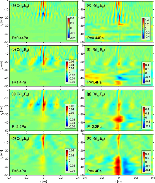
Figure 10. Contour plots of (a, b, c, d) C(Is, Eθ) and (d, e, f, g) R(Is, Eθ) as functions of τ and rp at (a, e) P = 0.44, (b, f) 1.4, (c, g) 2.2, and (d, h) 6.4 Pa.
Download figure:
Standard image High-resolution imageThe amplitude of the correlation function is strongly affected by the fluctuation amplitudes of the two signals in addition to their similarity. Thus, the cross-correlation coefficient, which is defined by the normalized C as  , is calculated. Figures 10(e)–(h) shows the cross-correlation coefficients drawn with the same color scale. It is found that there is no strong R in the periphery of |rp| > ∼ 30 mm at P = 0.44 Pa. In contrast, relatively strong correlation coefficients (R ∼ 0.4) are clearly observed at rp ∼ [−40, −32] mm at P = 2.2 Pa and |rp| > ∼ 30 mm at P = 6.4 Pa. The high-R structure in the former case (P = 2.2 Pa) seems to connect to the inner quasi-periodic structure (figures 10(c) and (g)), while the latter structure (P = 6.4 Pa) is separated from the inner structure (figures 10(d) and (h)). A positive correlation around τ ∼ 0 indicates the existence of radial transport due to the
Eθ
× B
drift. At P = 2.2 Pa, the radial range with high-positive R corresponds to a region where Is stops decreasing from the center and flattens (figure 5(b)). At |rp| > ∼ 40 mm, a positive correlation exists but suddenly decreases (R ∼ 0.2). In contrast, at rp ∼ −40 mm in the P = 1.4 Pa case, where the dip of the Is profile is shown in figure 5, weak negative and positive correlation coefficients are observed at τ ∼ 0 and τ < 0, respectively (figure 10(f)). However, they are not reliable because of the low-Is plasma, as discussed later.
, is calculated. Figures 10(e)–(h) shows the cross-correlation coefficients drawn with the same color scale. It is found that there is no strong R in the periphery of |rp| > ∼ 30 mm at P = 0.44 Pa. In contrast, relatively strong correlation coefficients (R ∼ 0.4) are clearly observed at rp ∼ [−40, −32] mm at P = 2.2 Pa and |rp| > ∼ 30 mm at P = 6.4 Pa. The high-R structure in the former case (P = 2.2 Pa) seems to connect to the inner quasi-periodic structure (figures 10(c) and (g)), while the latter structure (P = 6.4 Pa) is separated from the inner structure (figures 10(d) and (h)). A positive correlation around τ ∼ 0 indicates the existence of radial transport due to the
Eθ
× B
drift. At P = 2.2 Pa, the radial range with high-positive R corresponds to a region where Is stops decreasing from the center and flattens (figure 5(b)). At |rp| > ∼ 40 mm, a positive correlation exists but suddenly decreases (R ∼ 0.2). In contrast, at rp ∼ −40 mm in the P = 1.4 Pa case, where the dip of the Is profile is shown in figure 5, weak negative and positive correlation coefficients are observed at τ ∼ 0 and τ < 0, respectively (figure 10(f)). However, they are not reliable because of the low-Is plasma, as discussed later.
4.4. Radial transport with Eθ × B drift
To estimate the typical vr, the conditional averaging (CA) technique is applied to the Langmuir probe signals at rp = [−40, −32] mm, which is outside the target skimmer radius and equips a high correlation at P = 2.2 Pa and P = 6.4 Pa. CA has also often been used in blobby-plasma transport studies [19, 24]. Because in this experiment, the measurement position is changed with time, the moving-normalized Is,  , is used as a reference signal for CA, as in previous studies [7, 25]. Here, the moving-averaged mean and standard deviation are defined as
  and
and  , respectively, where
  indicates the average with a sliding window. The width of the sliding window is set to 40 ms in time, where a high-frequency component at
  Hz becomes ∼0 in
  . Before using the moving normalization, a low-pass filter at f = 19 kHz is applied to remove a non-negligible discharge-power-supply noise at f = 20 kHz and its harmonics, as described above. Furthermore, to restore the unit of the reference signal,
  is defined. Similarly,
  is calculated with a low-pass filter at f = 200 kHz.
Figure 11 shows the CA results of Is', vr', which is derived from the CA of Eθ', and Is'vr', which is roughly proportional to the radial particle flux. In this calculation, 110/41/46/41 time points are identified at P = 0.44/1.4/2.2/6.4 Pa, respectively, when Isn exhibits positive spikes with peak amplitudes over 1.5. Then, Is' and Eθ' signals around the detected time points are extracted and averaged in the same time domain along τ. In addition, because higher-frequency components exist at P = 0.44 Pa, the CA result with a low-pass filter at f = 50 kHz and a threshold value of 2.5 (111 time points) is additionally calculated and superimposed by the thin solid line.
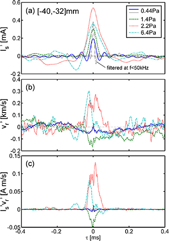
Figure 11. (a) CA results of Is', (b) vr', and (c) Is'vr' at rp = [−40, −32] mm at P = 0.44 (solid), 1.4 (dashed), 2.2 (dotted), and 6.4 Pa (dashed dotted). Only in the case of P = 0.44 Pa, the results of applying a different low-pass-filter frequency at f = 50 kHz are superimposed by thin solid lines.
Download figure:
Standard image High-resolution imageIt is observed that Is'vr' at P = 2.2 Pa has the maximum amplitude, while Is'vr' in the ionizing state at P = 0.44 Pa is sufficiently small, which is independent of the frequency of the low-pass filter. At P = 2.2 Pa, a positive spike of Is' with a duration of ∼0.2 ms accompanies a positive spike of vr' with a similar time scale and a typical radial speed of 200–300 m s−1. At P = 6.4 Pa, the Is' peak appears later than the vr' peak. This can be explained by the fact that the enhancement of the radial transport occurs near the recombination front, which is axially distant from the measurement position. The change in the plasma potential is transmitted in the parallel direction faster than that in plasma density, because the former and latter parallel speeds are determined by electrons and ions, respectively. Thus, the separated high-R structure in the periphery in figure 10(h) can be attributed to the localized radial plasma ejection and its parallel transport.
At P = 1.4 Pa, a negative vr' with a longer time scale than Is' spike is detected at τ > ∼ 0. As a result, Is'vr' becomes negative; however, the inward flux is not reliable. The longer-time-scale fluctuation in vr' can be explained as follows. Under this condition, because Is is quite small (figure 5), the plasma is very weak after the blob-like events pass the probe head. As an extreme condition, if there is no plasma, the time constant of the voltage change is determined by the resistance and capacitance in the probe circuit. Considering the input resistance of the analog-to-digital converter (1 MΩ) and the capacitance of the coaxial cable (∼1 nF per 10 m), the time constant becomes too long (>1 s with dozens of meters of the coaxial cable). Under this condition, if there is a difference in the time constants of two Vf measurement circuits, Eθ' and vr' would have finite values after changing the probe voltage over a long time scale after the passing of the blob-like events. Outward transport is not confirmed at P = 1.4 Pa.
The above analyses indicate that an enhanced radial transport exists in the recombination front where the ion-flux profile broadening is observed, as in the previous study conducted on NAGDIS-II [8]. To investigate the dependence on the radial position, the CA analysis is also applied at rp = [−22, −14] (94 time points) and [−30, −22] mm (63 time points) at P = 2.2 Pa, as shown in figure 12. The former and latter positions correspond to the region where the quasi-periodic fluctuation is clearly observed in figure 10(c) and the intermediate region between the former region and high-R region in figure 10(g), respectively. We can find a quasi-periodic Is' fluctuation, positive vr', and largest Is'vr' at rp = [−22, −14] mm. By increasing |rp|, the peak amplitude of Is'vr' decreases. In contrast, the vr' amplitude becomes the highest at rp = [−40, −32] mm. This might be because blob-like structures with large radial velocities are selectively transported to the periphery.
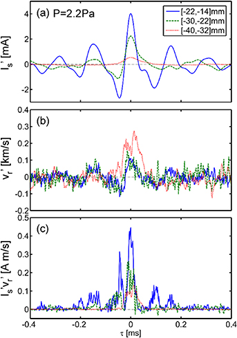
Figure 12. (a) CA results of Is', (b) vr', and (c) Is'vr' at rp = [−22, −14] (solid), [−30, −22] (dashed), and [−40, −32] mm (dotted) at P = 2.2 Pa.
Download figure:
Standard image High-resolution image5. Spatiotemporal behavior in the recombination front
Unlike the Langmuir probe, the fast framing camera is beneficial for measuring a wide range of fluctuations simultaneously without disturbance. The spatiotemporal behavior of Iem at P = 2.2 Pa in the recombination front, where the radial transport flux is the largest in figure 11(c), is investigated with electrostatic signals in this section.
5.1. Raw and filtered emission intensity fluctuations
Figure 13(a) shows a contour plot of  at zc = −10 mm as functions of t and rc. In the drawn time period, there are several radially elongated structures beyond the target skimmer radius with positive
  , which correspond to radial ejection events. Between rc ∼ −15 and 15 mm,
  is anti-phase, agreeing with the above prediction that the mode number of the f ∼ [3.5, 10] kHz component at rp ∼ [−25, −10] mm is m = 1. In addition, this fluctuation appears to be synchronized with the fluctuation around the radial center, whose mode number is m = 0.

Figure 13. (a) Contour plot of  at zc = −10 mm as functions of t and rc at P = 2.2 Pa. Time series of Iem (solid), IemL (dashed), and IemL + E(IemH)L (dotted) at (b) rc = 0, (c) −15, and (d) −30 mm. Time series of (e) Is (solid), IsL (dashed), IsL + E(IsH)L (dotted), (f) Itgt (solid), ItgtL (dashed), and ItgtL + E(ItgtH)L (dotted).
Download figure:
Standard image High-resolution imageThe horizontal slices of figure 13(a) at rc = 0, −15, and −30 mm are shown in figures 13(b)–(d) as a function of t. The low-pass Iem at f < 3.5 kHz, IemL, is also superimposed by green dashed lines in these figures. Here, f = 3.5 kHz lies roughly between the m = 1 rotation component and the m = 0 little maximum around the radial center; thus, IemL reflects the m = 0 frequency component. The IemL at rc = 0 in figure 13(b) appears to have an anti-phase relationship with that at rc = −30 mm in figure 13(d), while the IemL amplitude at rc ∼ −15 mm is small, as shown in figure 13(c).
Figures 13(e) and (f) shows the time series of Is at rp = −50 mm and Itgt. Similar to IemL, their low-frequency components, IsL and ItgtL, are overplotted by green dashed lines. The time series of Is shows non-simple behavior, but IsL seems to be correlated with IemL at rc = −30 mm with a time delay. In contrast, Itgt and ItgtL are quite similar to Iem and IemL at rc = 0, respectively.
5.2. Cross-correlation between emission intensities and electrostatic signals
Figure 13 shows the occurrence of several events within a short period of 2 ms. To clarify the spatiotemporal behaviors of the m = 0 and 1 modes over a longer period, a cross-correlation analysis is applied with the electrostatic signals at t = [2.3, 2.5] s under a steady-state condition.
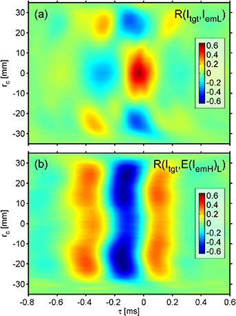
First, the cross-correlation coefficient between Is at rp = −50 mm and Iem,  , is investigated, as shown in figure 14. Here, a low-pass filter at f = 19 kHz is applied to Is before the correlation analysis to remove the power-supply noise. The maximum correlation (R ∼ 0.4) is detected at rc ∼ −28 mm when τ ∼ −0.3 ms, and this positive-correlation structure connects to the far peripheral region. This highest R position corresponds to the intermediate radial region (rp = [−30, −22] mm) in the CA analysis result (figure 12), which is just outside the region where the quasi-periodic fluctuation is observed. This means that the plasma ejection originates from the enhanced quasi-periodic fluctuation with m = 1 and reaches the far edge region at rp = −50 mm in ∼0.3 ms. At |rc| > 30 mm, R in figure 14 decreases but an internal electric field, which drives the radial transport, is maintained, as shown in figure 12. In addition, a negative correlation is detected at rc ∼ 0 when the maximum correlation is observed at τ ∼ −0.3 ms in figure 14.

Figure 14. Contour plot of  as functions of τ and rc at P = 2.2 Pa, where rp = −50 mm. A low-pass filter at f < 19 kHz is applied to Is before the correlation analysis.
Download figure:
Standard image High-resolution imageTo understand in detail each mode relationship, the cross-correlation coefficient between Itgt and IemL,  , is investigated, as shown in figure 15(a). Here, a low-pass filter at f = 19 kHz is applied to Itgt before the correlation analysis, in the same way as that in figure 14. A maximum correlation coefficient in
  is detected at rc ∼ 0 when τ ∼ −0.04 ms (R ∼ −0.6). Thus, a decrease in IemL around the radial center corresponds to the ion-flux reduction at the target with a time lag of tens of microseconds. In contrast,
  has negative peaks around |rc| = 24 mm at the same τ, meaning that the IemL radial profile becomes flatter when Itgt decreases. In contrast, at τ ∼ −0.3 ms, correlations with opposite signs to those at τ ∼ 0 are confirmed. This indicates that the IemL profile becomes steep before the profile flattening.
Figure 15. Contour plots of (a)  and (b)
  as functions of τ and rc at P = 2.2 Pa. A low-pass filter at f < 19 kHz is applied to Itgt before the correlation analysis.
Download figure:
Standard image High-resolution image
To reveal the amplitude behavior of the m = 1 mode, the Hilbert transform is applied, which can extract the envelope component of the fluctuation, E, from the absolute value of the analytical signal [7, 26, 27]. First, a high-pass filter at f > 3.5 kHz is applied to Iem (IemH), and then, its envelope, E(IemH), is calculated. After that, a low-pass filter at f < 3.5 kHz is applied to the envelope, E(IemH)L. The low-pass envelope plus low-pass signal, IemL + E(IemH)L, at each rc is superimposed in figures 13(b)–(d) with a magenta dotted line. Similarly, IsL + E(IsH)L and ItgtL + E(ItgtH)L are overplotted in figures 13(e) and (f), respectively. In figure 13(c), we can observe that E(IemH)L detects the enhancement of the m = 1 mode, particularly at rc = −15 mm.
Figure 15(b) shows the cross-correlation coefficient between Itgt and E(IemH)L,  , where a low-pass filter at f < 19 kHz is applied to Itgt before the correlation analysis. Strong negative correlations in
  are observed at |rc| ∼ [10, 25] mm when τ ∼ −0.15 ms (R ∼ −0.6). Moreover, at τ ∼ −0.4 and 0.1 ms, positive correlations (R ∼ 0.4) are observed within the same radial range. This indicates that the m = 1 fluctuation becomes strong just before the Itgt reduction and the m = 1 envelope amplitude oscillates quasi-periodically.
Because IemL and E(IemH)L are shifted by approximately a quarter period of f ∼ 1.5 kHz from that in figures 15(a) and (b), a predator-prey-like relationship exists between the m = 0 and 1 modes. The analysis results can be interpreted as follows: before the Itgt reduction at τ = 0, a weakening of the m = 1 mode occurs at τ ∼ −0.4 ms, and then, the IemL profile sharpens at τ ∼ −0.3 ms. After that, the m = 1 mode strengthens at τ ∼ −0.15 ms and elongates toward the periphery, which leads to radial transport. At τ ∼ 0, owing to the radial plasma ejection from the plasma column, the IemL profile becomes flatter, and the m = 1 mode weakens again at τ ∼ 0.1 ms. Although Iem is simply a line-integrated emission signal, considering the strong correlation between Iem and electrostatic signals, Iem reflects the motion of coherent structures. In addition, considering the phase relationship between changes in the m = 0 mode profile and the m = 1 mode intensity, the m = 1 mode can be directly or indirectly driven by the radial gradient of the plasma profile.
A strong relation between the m = 0 and 1 modes was also reported in previous experiments conducted on NAGDIS-II [7, 9] and a three-dimensional numerical simulation [28]. However, a clear quarter-period shift between the two modes and their quasi-periodicity is observed for the first time in this study.
6. Summary and discussion
Spatiotemporal behaviors of fluctuations and cross-field transport in Magnum-PSI detached He plasmas were analyzed. By using a reciprocating Langmuir probe, ion-flux profile broadening and an increased fluctuation in the periphery were observed around the recombination front, which is defined as the region where the line-emission intensities from highly excited states are strong. Within the target skimmer radius, the Er × B rotation of the m = 1 mode was identified. The fast framing camera measurement revealed that the amplitude of the m = 1 mode fluctuated with about a quarter-period shift from the m = 0 mode, which made the emission profile flatter or sharper across the magnetic field. The ejected plasma behind the target skimmer was correlated with the enhanced m = 1 mode and the coherent structure was transported radially outward by the Eθ × B drift. This structure reached a position with a radius of ∼50 mm that was outside the flux tube connected to the target plate. As a result, the ion flux flowing into the target plate decreased during the enhanced radial transport. Many of the results obtained here are similar to those of previous studies conducted on another linear plasma device NAGDIS-II; a clear quasi-periodic predator-prey-like feature with the quarter-period shift between the two modes was first observed in Magnum-PSI.
Behind the target skimmer, the ejected coherent structures were transported by the Eθ × B drift. In linear devices, there was no strong magnetic field gradient and curvature, which are considered to generate Eθ inside blobs in tokamak devices. One of the possible effects of generating Eθ in this study is the neutral wind effect [9, 29, 30]. Owing to the enhanced volume recombination in the recombination front, several neutrals in highly excited states, besides the ground state, were generated near the radial center. These neutrals were not trapped by the magnetic field and provided the outward force (Fr ) to the edge plasmas. Then, the Fr × B drift generated Eθ in coherent structures at the periphery.
At P = 1.4 and 1.8 Pa, which are under the plasma condition between the ionizing plasma and recombination front at the TS axial position, a dip was observed at rp ∼ [−40, −32] mm. Under this pressure condition, a recombination front existed between the TS axial position and the target plate. Considering that the enhancement of the radial transport was localized in the recombination front, like NAGDIS-II [8], the cross-field transport occurred just in front of the target plate. Because the target structure is a strong ion-particle sink along the magnetic field, Is at the TS axial position opposite to the target plate decreased. In contrast, outside the target-plate radius, there was a floating target skimmer and a vessel wall with a longer distance. Therefore, the difference in particle sinks at different radial ranges is attributable to the existence of the dip. In addition, a sudden decrease in  was observed outside the dip position in figure 10(g). The reason behind this is unknown, but the plasma that remains for a long time due to the small particle sink may weaken the azimuthal electric field by creating a long arc-like structure in the azimuthal direction.
Because this study is an initial step toward extending to the ITER-relevant condition, measurements under the stronger magnetic field condition are essential. In this study, a strong correlation between the electrostatic and emission fluctuations was confirmed. Therefore, by locating the Langmuir probe behind the target skimmer, where the heat load was small, and using a fast framing camera viewing inside the target skimmer, the transport characteristics can be investigated even under the ITER-relevant condition. Furthermore, complementary studies with magnetic confinement devices are required to reveal the geometric effects and forecast the transport characteristics in future devices.
In hydrogen-isotope plasmas, an additional volume-recombination process, called molecular activated recombination, occurs even at electron temperatures above 1 eV [31, 32]. This would act not to localize the recombination front along the magnetic field compared to the He plasma, in which only the electron-ion recombination process becomes dominant at less than 1 eV. If the recombination and the neutral-flow effect are important for generating Eθ, the difference in the recombination processes would significantly change the transport-occurring region and its characteristics. In addition, most of the plasma particles are hydrogen isotopes in future fusion devices. Therefore, transport studies on hydrogen-isotope plasmas and comparison with results obtained for He plasma are future work in Magnum-PSI.
Acknowledgments
We greatly appreciate Magnum-PSI team for performing fruitful experiments and discussions. This work was supported by JSPS KAKENHI (16H06139, 16H02440, 17KK0132, 18KK0410, 19K14686), NIFS Collaboration Research program (NIFS17KUGM120, NIFS19HDAF003), the Naito Research Grant, NIFS/NINS under Young Researchers Supporting Program (UFEX106), and NINS program of Promoting Research by Networking among Institutions (01411702). The Magnum-PSI facility at DIFFER has been funded by the Netherlands Organisation for Scientific Research (NWO) and EURATOM. DIFFER is part of the institutes organisation of NWO and a partner in the Trilateral Euregio Cluster TEC.