

Abstract
We present the first parallel electron transport results obtained using the newly developed 1D transport code SOL-KiT. With the capability to switch between consistent kinetic and fluid models for the electrons, we explore and report the differences in both equilibrium and transient simulations. Significant kinetic effects are found during transients, especially in the behaviour of the electron sheath heat transmission coefficient, which shows up to an eightfold increase. Equilibria are obtained for an input power scan with parameters relevant to medium size tokamaks. Detached equilibria are found to persist to higher input powers when electrons are treated kinetically. Furthermore, non-monotonic behaviour of the electron sheath heat transmission coefficient is observed in the power scan, with values being up to 40% above the classical value. We discuss the implications of the presented results to potential modelling decisions, as well as possible extensions to the used model.
Export citation and abstract BibTeX RIS

Original content from this work may be used under the terms of the Creative Commons Attribution 4.0 license. Any further distribution of this work must maintain attribution to the author(s) and the title of the work, journal citation and DOI.
1. Introduction
The Scrape-Off Layer (SOL) is the region of open field lines in Magnetically Confined Fusion devices, through which the energy and particles which escape the fusion core travel to the plasma-facing components of the reactor. Transport occurs along and across the open field lines of the SOL, and understanding it is a key issue for future reactor design [1]. Parallel transport carries energy and particles from the hot upstream to the divertor targets, and determines, in combination with other physical processes (such as atomic and molecular physics), the divertor heat load. Fluid modelling is often adopted for numerical expediency when tackling the problem of parallel transport, utilizing the classical results of Braginskii [2], and allowing modification of the heat flux through the use of flux limiters [3]. However, as the parallel direction of the SOL is characterized by large gradients in both temperature and density (and thus collisionality), kinetic effects can modify transport properties, and have been proposed as potential causes of discrepancy between fluid simulations and experimental results [4].
Previous numerical studies of kinetic effects in the SOL have been performed with a wide array of codes, including both PIC [5, 6] and finite-difference codes [7–12]. These studies report the impact of kinetic effects in various aspects of parallel transport, including the modification of the parallel heat flux and atomic rates [9], as well as effects on the properties of the plasma sheath. Havlíčková et al [13] compare the results of different fluid and kinetic codes during simulations of Edge-Localized Modes (ELMs), and report sensitivity of target heat flux peak values to applied flux limiters. Large gyrokinetic codes have also been used to study full edge turbulence [14, 15]. However, such large codes need support for lower dimensional studies, and the study we present here uses a faster and flexible code developed with that aim in mind.
Our goal in this study is tackling the comparison between a fluid and kinetic model of parallel electron transport, with a focus on extracting kinetic effects. For this purpose, we avoid very (machine-)specific scenarios popular in the literature, and instead vary the input power into the SOL while keeping other parameters (such as total density) fixed. We use the newly developed transport code SOL-KiT (Scrape-Off Layer Kinetic Transport) [16], where electrons can be treated as either a fluid or kinetically, while ions are treated as a fluid. SOL-KiT also includes a basic self-consistent treatment of atomic processes in a pure deuterium plasma.
We start by presenting the basics of the SOL-KiT model, before moving on to the first results. The input power has been scanned in both fluid and kinetic modelling, and the equilibrium results are reported and compared to examine kinetic effects in steady state. The parameters used are relevant to medium size tokamaks (MSTs), where a current research concern is the interaction of transients, such as ELMs and other perturbations, with detachment, the plasma state in which the divertor target is effectively shielded by the presence of a neutral cloud [17]. Transients are launched on the simulated equilibria, and the resulting evolution of various quantities, including the temperature at the target, are presented, showing significant kinetic effects. We close by summarising the electron transport model used, noting its limitations and considered extensions, and discussing the results obtained in this study.
2. The SOL-KiT model
The SOL system of interest is represented as a straightened-out 1D SOL in slab geometry, with the x-axis being along the magnetic field line. The upstream position x = 0 is taken to denote the location of the (reflective) symmetry plane, while the downstream boundary is at the entrance of the target sheath.
We solve equations for the electrons, ions, atomic neutrals, as well as the parallel electric field. The ions are treated as a fluid, while neutrals obey a diffusive-reactive collisional-radiative model. For the electrons we can use either fluid or kinetic equations, with care taken to keep the two models consistent with each other. This allows for clean comparisons between them, which are the focus of this study. We refer to consistency as the fact that the fluid model is derived by taking the appropriate moments of the kinetic equations used, and utilizing the same atomic data. The concept of consistency is discussed further in the appendix.
2.1. Fluid and neutral equations
The three moment equations for the electrons, as solved by SOL-KiT (for conservative forms see appendix), are
where k is the Boltzmann constant, E is the electric field in the parallel direction and  is the ionization and recombination particle source. ne and Te are the electron density and temperature, respectively, while ue is the parallel flow velocity of the electron fluid. The friction
  is taken from Braginskii [2] with
  and
and  , where the τe is the electron-ion collision time [2]. Ren is the total electron-neutral friction, calculated using a slowly drifting Maxwellian for the electrons (see appendix).
The heat flux  is given by
  and
and  , with
  being the classical Spitzer-Härm value. The energy loss/gain due to inelastic collisions and the external heating in the temperature equation is given by
  . For a more detailed discussion of these terms the reader is referred to the appendix.
For the ions (of charge Ze) we take both  (quasi-neutrality), and assume
  (see section 3 for more on the effect of this approximation). This leaves just the ion momentum equation
where Rie can be calculated using momentum conservation in ion-electron collisions. Charge exchange friction RCX is given by
where the sum is over neutral atomic states, and we simplify the expression by approximating the ions as cold, and the neutrals as cold and stationary. The constant charge exchange cross sections are approximated by the low energy values for hydrogen from Janev [18]
The electric field comes from Ampère-Maxwell's law
which is reduced to only containing the displacement current. This might appear unusual, but note that other similar Vlasov-Fokker-Planck codes, both explicit [19, 20] and implicit [21], include the displacement current or the full Ampère-Maxwell's law in their calculation of the electric field. In practice, however, given that the displacement current is negligible on time-scales of interest, the above equation acts as a current constraint, allowing the pressure gradients and collisional friction to set the electric field.
Finally, the atomic state distribution of the neutrals must be tracked. This is done using a diffusive-reactive model
where we use moments of the electron distribution function (Maxwellian in fluid model) to calculate the ionization and (de)excitation rates K, as well as three-body recombination rates α. Neutrals are taken to be cold compared to the electrons for all rate calculations. The required atomic data are all taken from Janev [18] and NIST [22]. Data for spontaneous emission rates A are included up to state b = 20; however, this truncation should not introduce a substantial error for higher states, as those are primarily collisionally dominated. Finally, we include radiative recombination β as a function of temperature [18]. In order to include diffusion, we use the classical 1D diffusion coefficient
for the sake of which we treat neutrals as having a thermal velocity vtn, and assume that the diffusion is due to elastic collisions between ions and ground state neutrals and charge-exchange collisions with the ions. σel is the approximate elastic collisions cross-section based on the Bohr radius  (usually negligible compared to the charge-exchange contribution), and n1 being the ground state density. The neutral temperature used to calculate vtn is a free parameter (see section 3).
At the sheath boundary, ions reach the sound speed (as per the Bohm criterion). In the fluid case, ambipolar flux is assumed  , where
  and
and  , and the Z = 1 case (relevant to the SOL) is treated. The sheath heat transmission coefficient [17] in the transmitted sheath heat flux

is set to  , with the RHS evaluated at the entrance to the sheath. This corresponds to the classical result, with the electrons at the entrance of the sheath obeying a cut-off Maxwellian distribution, and qsh being the resulting (total) heat flux due to such a distribution. The cut-off represents the missing electrons, i.e. those electrons that can overcome the sheath potential and are lost to the target while others are reflected [17] (see section 2.2.5 for the kinetic case). Neutrals are recycled with flux
  , where R ≤ 1 and Γi is the ion flux to the target.
2.2. Electron kinetic equation
Starting from the classical 1D kinetic equation for the electrons

where the RHS contains all of the collision and source operators, we expand the distribution function in spherical harmonics. We follow the approaches used in the codes KALOS [19] and OSHUN [20] and write the expansion as
where θ is the angle between the velocity vector  and the x-axis, which is aligned to the magnetic field, ϕ is the azimuthal angle, and
  are associated Legendre polynomials. In order to lighten notation, x and t dependence of f is implied wherever omitted. Since the model is 1D and azimuthally symmetric, we set m = 0, and the expansion reduces to a Legendre polynomial expansion, and m is dropped from the notation. The choice of spherical/Legendre harmonics as the basis was informed by the fact that they are the eigenfunctions of pitch-angle scattering operators, allowing for simplified treatments of collisions. The standard fluid moments are also conveniently related to particular harmonics, with density and energy being moments of f0, and the various fluxes moments of f1 (see appendix for more details).
By projecting equation (10) onto the Legendre basis, equations of the following form are obtained for the distribution harmonics fl

where  and
and  are the advection (Vlasov) terms, and
  are all other operators. While the derivations (and some of the full forms) of these operators are beyond the scope of this paper, we give a brief overview below, and direct the reader to the literature where appropriate. The full details of the SOL-KiT model, as well as code numerics and benchmarking, will be the subject of another publication [16]. However, for the sake of clarity of the presented results, we briefly discuss some numerical aspects of the code at the end of this section.
2.2.1. Vlasov terms.
The spatial advection term (advection in the x-direction), for a given harmonic l is
while the velocity space advection [19] is given by
As can be seen from these equations, Vlasov terms couple different harmonics through either spatial gradients or the electric field.
2.2.2. Coulomb collision terms.
We consider the effect of Coulomb collisions on the distribution function f of particles with mass and charge m and q = ze, respectively, colliding with particles of mass and charge M = µ m and Q = Ze, which have a distribution F. Following the formalism of Shkarofsky et al [23], we start with the Rosenbluth form of the Fokker–Planck collision operator
where  and
and ![$\Gamma_{zZ} = (zZe^2)^2\ln\Lambda/[4\pi(m_s\epsilon_0)^2]$](https://content.cld.iop.org/journals/0741-3335/62/9/095004/revision2/ppcfab9b39ieqn24.gif) . The Rosenbluth drag and diffusion coefficients are respectively
. The Rosenbluth drag and diffusion coefficients are respectively  and
and  . We linearize the collision operator in the anisotropic component of the distribution functions (
 ,
,  ). After expanding the distribution function and the Rosenbluth coefficients in harmonics and using the integrals [23]
we get for l = 0
while for l > 0
where the C coefficients are available in the literature [20]. For electron-electron collisions µ = 1, and the collision operator for the isotropic part of the distribution function [21, 24] is
where the drag and diffusion coefficients are
The electron–electron collision operator for l = 0 is important for the proper relaxation of the electron distribution function to a Maxwellian. For the sake of brevity, we omit the electron-electron collision operator for higher harmonics (see [20, 23]), and note only that the l = 1 component redistributes momentum among the electrons.
As  , no l = 0 component for the electron-ion collision operator is used. For higher harmonics and stationary ions (
 ) equation (21) reduces to the following eigenfunction form
which is pitch-angle scattering. The eigenvalue is negative, so this operator dampens harmonics with high l. Thus one can truncate the expansion at some finite l. When ions are not stationary but their velocity is much smaller than the electron thermal velocity (the situation we expect in the SOL), we can approximate their distribution as a Dirac delta  , which allows us to treat the plasma close to the divertor target.
2.2.3. Boltzmann collision terms.
To model electron-neutral collisions we use the Boltzmann collision integral for collisions between species s and 
where primed velocities denote values before a collision, and σ is the appropriate differential cross-section. Using a standard procedure for particle-conserving (e.g. excitation) inelastic collisions [23, 25, 26], we get
where  , and σTOT is the integral cross section, while
where Pl are Legendre polynomials.
For ionization (and other collisions that do not conserve total number of particles), we take the simplest possible approach and add (or remove) electrons to (from) the lowest velocity cell [7], using
where  is the particle conserving part, and
For inverse processes we use the principle of detailed balance [27, 28] to obtain cross-sections. For deexcitation (from state i to j) this is
where gi and gj are statistical weights (for hydrogen  ). Velocities
  and v are related through the excitation energy. For 3-body recombination we use the statistical weights of a free electron gas to get
where h is the Planck constant, and  is the ion ground state statistical weight (for hydrogen
  ).
).
2.2.4. Electron heating operator.
The implemented diffusive heating operator has the form
where Θ(Lh−x) designates the heating region. If we assume a spatially uniform heating we get

where Wh(t) is the heat flux entering the SOL over length Lh. This is related to the fluid model heating Qext as  .
.
2.2.5. Divertor target boundary condition with Legendre polynomials.
Similarly to the fluid case, we set flow to be ambipolar at the sheath entrance. We then use the logical boundary condition [29], which assumes that all electrons with  are lost, while all others are reflected. This translates to having a cut-off in the electron distribution function at
  . The challenge comes in decomposing this condition in Legendre polynomials. Fortunately, the number of required harmonics to capture the basic behaviour is usually not prohibitively high, with l = 1 enough for the condition to be satisfied, although higher harmonics will improve accuracy. We omit the derivation of the decomposition, and note that the 'cut-off' distribution harmonics can be written as a linear combination of known harmonics
where  is the transformation matrix containing the details of the cut-off. With the distribution function form known, the ambipolarity condition is
where ni,sh is the density at the sheath boundary, and ui,sh is the ion velocity at the boundary, given by the Bohm condition ![$u_i \geq c_s = [k(T_e+T_i)/m_i]^{1/2}$](https://content.cld.iop.org/journals/0741-3335/62/9/095004/revision2/ppcfab9b39ieqn44.gif) ,where Te is the electron temperature of the cut-off distribution, and Ti is the ion temperature. The ambipolarity condition gives vc, and with it the sheath potential drop
,where Te is the electron temperature of the cut-off distribution, and Ti is the ion temperature. The ambipolarity condition gives vc, and with it the sheath potential drop  .
.
2.3. Model numerics
As previously noted, the details of the numerical methods used in SOL-KiT will be the topic of another paper [16]. However, we present basic elements of the algorithm here to aid the presentation of results in the following sections.
SOL-KiT is a fully implicit 1D finite-difference code. Timestepping is done using a Backward Euler scheme. When switching between kinetic and fluid electrons, we simply restructure the model matrix to include elements calculated using the desired model. This does change the dimension of the matrix, as the kinetic model requires use of a velocity grid with number of cells Nv, as well as accommodating a number of harmonics up to lmax, whereas the fluid model needs only the staggered spatial grid with Nx cells.
Staggering of the spatial grid is simply performed by resolving the scalar (ne,Te,nb,f0, etc) quantities in cell centres, while vector quantities (E,ui,f1, etc) are given only on cell boundaries. For the simulations performed here, the spatial grid is logarithmic, with cells closer to the sheath boundary being smaller. This allows for better resolution close to the target, where spatial gradients are large. In all runs here Nx = 64.
The velocity grid used in the kinetic runs presented here is geometric, and velocity is normalised to vth,0 - the electron thermal velocity for a reference temperature of 10 eV. This approach allows for properly capturing low energy electrons and their dynamics, as well as making sure the high energy tail is resolved. We use Nv = 80, with lmax = 1 (the diffusive approximation [30]), and take the smallest velocity grid cell width to be dv = 0.05vth,0, while resolving velocities up to ≈ 12vth,0. While the choice of lmax = 1 is a relatively crude approximation, leaving out effects like pressure anisotropy, it is enough to capture the basic dynamics of fluxes. See the discussion in section 5 for more on this.
To achieve speed-up during high collisionality kinetic equilibrium runs, a self-consistent coupling scheme between the two models was employed, allowing the fluid model to be run using the corrected transport coefficients obtained with the kinetic model. The details of this coupling scheme will be presented elsewhere.
Finally, in order to capture the collisional dynamics during kinetic simulations of transients, we use a timestep that resolves the collision times in the system (see section 4).
3. Simulation setup and equilibrium results
We set up the simulations in the following way. The length of the domain is L = 10.18 m, with the heat source injecting energy over Lh = 3.75 m upstream. The total (plasma and neutral) line-averaged density is kept at  by utilizing 100% recyling (R = 1). Recycling produces deuterium atoms with temperature Tn = 3 eV (mimicking Franck-Condon enhancement [17]), and we track a total of 30 atomic states. The choice to track this many was made because a noticeable difference was observed between test runs with 30 and those with fewer states. This is likely due to the fact we do not use any collisional-radiative closure for highly excited states (a similar approach to that in Reference [9]).
The first set of simulations we describe is an input power scan using either fluid or kinetic electrons. Note that all equilibrium results presented here were obtained by running the code until there were no significant transients remaining (local Mach number in the upstream region does not exceed M = 5 × 10⁻³). As such, the initial condition influences only the time required to reach equilibrium. The effective input power flux was varied from 1MW/m2 to 6MW/m2. The input power range used allows us to consider qualitatively different regimes, while staying in a parameter range relevant to MSTs. Upstream collisionalities  (where λ is the electron-electron mean free path [17]) are in the range of ν*≈ 10 − 26 for the obtained equilibria.
Figure 1 shows temperature profiles for several input powers, with both the fluid and the kinetic equilibria presented. As can be seen from the difference between the upstream (x = 0) and downstream (target) temperatures, the fluid electron temperature profiles flatten as input power is increased, while the kinetic profiles maintain a stronger gradient. Remembering the strong temperature dependence of the conductivity, the flattening of fluid equilibria indicates potential agreement with the Two-Point Model [17], confirmed below (see figure 5 and accompanying discussion). The agreement between fluid and kinetic equilibrium profiles is observed to decrease as input power is increased and collisionality drops. The kinetic profiles also have systematically lower target temperatures, while upstream temperatures are slightly higher than or around the fluid model values. The isotropic diffusive heating operator produces a small imprint in the kinetic temperature profiles, evident from the change in slope around x = 3.7 m (however, the effective heating power is the same as in the fluid runs). A minor uptick (change in gradient sign) in the electron temperature at the target is present for higher power runs. While practically invisible in figure 1 due to being localised close to the target, the effects of the uptick are visible in other quantities (see below, figure 4). We expect this to be the consequence of taking  , as the lower collisionality should decouple electron and ion temperatures, leading to different pressure and electric field profiles, and this is not captured in our model.
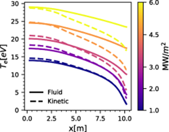
Figure 1. Equilibrium temperature profiles for a few representative powers from scan for both the fluid and the kinetic electron models.
Download figure:
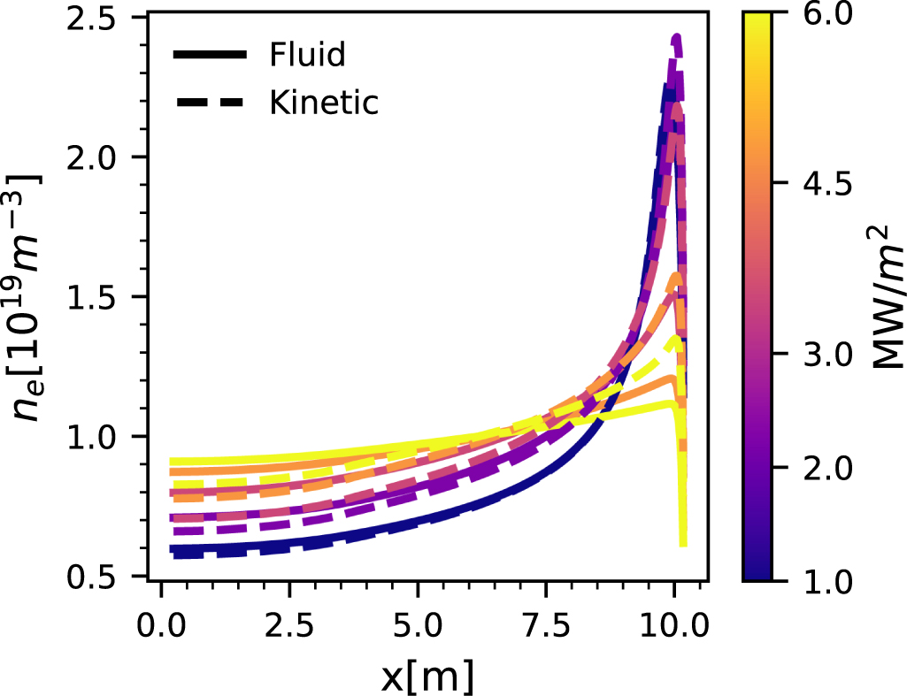
Standard image High-resolution imageFigure 2 shows the density profile behaviour for these runs. As the power increases the density flattens, with the fluid runs showing a higher degree of flattening compared to the kinetic runs. This agrees with the increased steepness of kinetic temperature profiles observed in figure 1, as well as decreased target temperatures in those runs. The flattening of the electron density profile is accompanied by the depletion of neutrals, evident from the ground state neutral density shown in figure 3. Looking at the extent of the neutral cloud in figure 3, it can be seen that as the power is increased the cloud is forced closer to the target. Note that runs with kinetic electrons show an increased neutral density, likely due to lower temperatures near the target.

Figure 2. Density profiles for runs from figure 1 - as the power is increased the profile begins flattening.
Download figure:
Standard image High-resolution image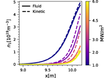
Figure 3. Ground state neutral density profiles for runs from figure 1 - as input power grows the neutral population diminishes.
Download figure:
Standard image High-resolution imageThe increased steepness of temperature profiles in simulations with kinetic electrons can be readily explained by looking at the ratio of the calculated conductive heat flux q to the classical Spitzer-Härm value qT based on the local temperature profile . This is shown in figure 4, where we see that the heat flux upstream is suppressed (we also see again the imprint of the heating operator). Near the target the heat flux is weakly enhanced for the lower heating powers, and the slight temperature uptick at the boundary causes the ratio to go negative, since the calculated Spitzer-Harm heat flux changes sign. These results are qualitatively similar to those obtained by Batishchev et al [7] using a code where all species were treated kinetically, with the discrepancies seemingly due primarily to the use of an isotropic heating operator and the  approximation.
In order to further illustrate the differences between the kinetic and fluid model, we write here a simple Two-Point Model (2PM) [17] result for the temperature where an input heating flux qin is distributed along a heating length Lh
where κe was calculated by taking a Coulomb logarithm of 12. The upstream and downstream temperatures Tu and Td are sampled in the first and last spatial cells, respectively. We plot  as a function of input power in figure 5 for both the obtained fluid and kinetic equilibria, as well as the above 2PM. The fluid results appear to agree well with the 2PM, although the densities do not obey the predictions of the model
  , as shown in figure 6. This is due to the presence of sources and sinks, and the resulting change in pressure balance, with the discrepancy between fluid and kinetic results here due to the lower target temperatures in the kinetic case. The kinetic simulations also show a systematic increase of the calculated difference
  in figure 5, which points to a reduction in the effective conductivity
  in the above model. This is the consequence of flux suppression -
  . However, note that the details of the flux suppression or enhancement depend on the input power and location within the system. As such, there appears to be no simple way (e.g. flux limiters) to capture the entirety of the kinetic effects.

Figure 4. Ratio of calculated conductive heat flux to the classical local value. Upstream heat flux is suppressed, while lower input power runs show flux enhancement near the boundary. Negative values of the ratio are due to the temperature uptick - most likely a consequence of the  approximation.
Download figure:
Standard image High-resolution image
Figure 5.  as a function of input power for the obtained equilibria. The Two-Point Model result is given as the dashed line, and appears to agree well with the fluid simulation results. Kinetic simulations show a systematically increasing gap, further illustrating the effect of flux suppression.
Download figure:
Standard image High-resolution image
Figure 6. 2 as a function of input power for the obtained equilibria. Both the fluid and the kinetic results show a loss in downstream pressure characteristic for momentum loss, and do not agree with the predictions of the Two-Point Model.
Download figure:
Standard image High-resolution imageFigure 7 shows the l = 0 harmonic in the last cell before the boundary for kinetic runs with several different input powers. Comparing it to a Maxwellian distribution of equivalent density and temperature reveals a 'hot' tail of electrons, which modify the transport properties as seen above. This is due to the fact that heat carrying electrons, those electrons which contribute most to the heat flux [10], can have energies  , so not many are needed to influence the heat flux. In order to quantify how much energy is carried by the fast electrons, the following quantity is calculated near the target
representing the total heat flux carried by those electrons above some threshold energy  . Note that f1, which governs the heat flux, is a strong function of f0 (this can be shown using simplified versions of the kinetic equations from the previous section). To determine the threshold energy (the energy at which the hot tail in figure 7 begins), the following two criteria were used:


where  is the equivalent Maxwellian to f0. This way, the effect of the kinetic correction on fast tail electrons is singled out by requiring the deviation of the distribution function from Maxwellian. Results for the percentage of heat flux carried by the tail electrons as well as the threshold energies are given in table 1. As can be seen from this data, even the lowest power equilibrium has fast tail electrons carrying a non-negligible fraction of the heat flux - more than 20%. Here the stronger kinetic effects seen in the steepening of temperature profiles in figure 1 for higher input power equilibria manifest themselves as a large fraction of heat flux carried by fast electrons.
Table 1. Percentage of the heat flux carried by tail electrons.
| qin (MW m−2) | 1 | 2 | 3 | 4.5 | 6 |
|---|---|---|---|---|---|
| %qfast | 21.44 | 38.61 | 51.33 | 61.87 | 65.15 |
| Ethresh[eV] | 13.4 | 27.6 | 41.7 | 72.3 | 100.8 |
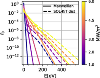
Figure 7. The l = 0 harmonic near the target sheath for kinetic electron runs for several input powers, as a function of electron energy. The solid line shows Maxwellians with equivalent density and temperature.
Download figure:
Standard image High-resolution imageFinally, we present results for the particle and energy fluxes into the target sheath. Figure 8 shows the variation of the particle flux into the sheath and the sheath heat transmission coefficient (see 9) with input power. A standard detachment criterion is the rollover of particle flux to the target during an upstream density scan. However, as we have performed an input power scan with total line averaged density constant, we expect rollover as input power is decreased, corresponding to increased collisionality. Indeed, at 3.5MW m−2 we observe the start of a flux rollover in the kinetic electron simulations, while the fluid case is different, as rollover happens around 2.5MW m−2. We interpret the particle flux rollover as the onset of detachment, and restrict equilibria to input powers below 4.5MW m−2 (i.e. up to a representative attached case) in the following section. An interesting feature is observed as input power is decreased from the highest value - an unexpected initial drop in target flux. However, this is readily explained by the fact that we choose to keep total density (plasma and neutrals) fixed, and there is an initial reduction of plasma available as more neutrals remain un-ionized.

Figure 8. The particle flux into the sheath and the sheath heat transmission coefficient for both the kinetic and fluid runs in the power scan. Rollover behaviour observed in both quantities.
Download figure:
Standard image High-resolution imageAs for the heat transmission coefficient in figure 8, note that for the fluid runs it is set to  , which results in γ ≈ 5. Around 3.0MW m−2 the coefficient experiences a rollover-like effect. This behaviour can be explained as follows. In the low input power limit we expect collisions to dominate and the regime to be well described with a fluid model, thus setting γe to its classical value. The high input power limit should produce a flat temperature profile, and with no gradients we again expect to return to the local value of ≈ 5. Thus if there is any change in γe we expect rollover-like behaviour at an intermediate input power. An explanation of why the heat transmission coefficient increases could be the same as for flux enhancement, i.e. the presence of hot electrons in the tail of an otherwise cold electron distribution. We note that similar non-monotonic behaviour, although during a pure collisionality scan, was observed with both the PIC code BIT1 [5] and the finite difference code KIPP [11].
4. Transient simulations
Transient simulations were performed by starting from the above equilibria, and increasing the input power flux to 45MW m−2 for ≈ 10 µs. After this the input power was returned to its original value for a further ≈ 10 µs, allowing the perturbation to relax. A similar perturbation setup has been used in the literature to model type III ELMs [7] in the SOL. We use only equilibria with input powers up to 4.5MW m−2, in order to capture representative attached as well as detached behaviour for both the fluid and kinetic runs. In order to resolve collisions properly, we set the timestep in these simulations to ≈ 3 ns. Since SOL-KiT allows moving from fluid to kinetic simulations, it is possible to launch a kinetic perturbation on a fluid background by initializing the electron distribution as a Maxwellian. This would significantly reduce run time, as fluid equilibria converge much faster. We explore this below, considering the three possible combinations of equilibria and perturbation physics, as presented in table 2.
Table 2. Possible combinations of equilibria and perturbations based on equilibrium and perturbation physics used.
| Fluid perturbation | Kinetic perturbation | |
|---|---|---|
| Kinetic equilibrium | NA | kinetic on kinetic |
| Fluid equilibrium | fluid on fluid | kinetic on fluid |
Figure 9 shows the evolution of the perturbation on the 1MW m−2 input power background for the various combinations in table 2. The two kinetic models (kinetic perturbation on kinetic/fluid background) agree well, and have steeper temperature variation than the fluid model from upstream to target, showing that there is less efficient heat transport, i.e. flux suppression, in the kinetic models. The fluid model has lower upstream and higher target temperatures, leading to an overestimation of target heat flux compared to the kinetic case. This sort of transient effect could contribute to erosion models that use a fluid plasma model potentially predicting a higher degree of wall damage.

Figure 9. Temperature profile evolution for perturbation launched on the 1MW m−2 background. The fully fluid model overestimates the target temperature, while the two kinetic simulations seem to agree well, with a higher upstream temperature than the fluid model during the perturbation.
Download figure:
Standard image High-resolution imageThe evolution of temperature at the target sheath boundary for several background input powers is shown in figure 10, for the fluid and fully kinetic case, respectively. As can be seen, the peak temperatures at the target in the kinetic case are up to almost two times lower than in the fluid case. However, the temperature decays faster in the fluid than in the kinetic model, which is most likely due to the suppressed upstream flux relaxing more slowly.

Figure 10. Evolution of the temperature perturbation at the target for several input powers. Presented are both a fluid perturbation and a kinetic perturbation on kinetic background.
Download figure:
Standard image High-resolution imageIt is useful to observe the evolution of the q/qT ratio during the perturbation. We focus on two locations, one near the middle of the domain, and one close to the target. These results are shown in figures 11 and 12. The midpoint ratio evolution indicates an initial bout of flux enhancement (compared to the equilibrium), after which the heat flux is heavily suppressed. We note here that the lowest power equilibrium has the strongest kinetic response to the perturbation, which is also visible in figure 12, where it experiences much greater enhancement compared to other equilibria. We expect this to be due to lower power equilibria having a much larger energy contrast between the local cold and the much hotter electrons coming from the upstream (see figure 13 below).

Figure 11. Ratio of calculated conductive heat flux to the local value during the kinetic perturbation run. Shown are several different background input powers at x = 5.29 m. After an initial period of enhancement, the flux is heavily suppressed.
Download figure:
Standard image High-resolution image
Figure 12. Ratio of calculated conductive heat flux to the local value during the kinetic perturbation run. Shown are several different background input powers at x = 10.09 m. Close to the target, heat flux enhancement dominates during most of the perturbation. Dashed horizontal line shows q/qT = 1 for reference.
Download figure:
Standard image High-resolution image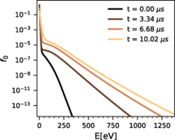
Figure 13. Evolution of the l = 0 harmonic near the boundary during the perturbation on the 1MW m−2 input power background (kinetic on kinetic background). This corresponds to the solid line in the first four subfigures of figure 9.
Download figure:
Standard image High-resolution imageThe evolution of the l = 0 harmonic in the last cell before the boundary is presented in figure 13, corresponding to the solid line in the first four subfigures of figure 9, with the perturbation being launched on the 1MW m−2 input power kinetic background. As expected, the perturbation manifests itself as a growing tail of energetic electrons.
We now turn to the evolution of the sheath properties, namely the sheath heat transmission coefficient and the sheath potential drop. Presented in figures 14 and 15 are the heat transmission coefficient and sheath potential drop during the kinetic perturbation for several input powers of the kinetic equilibria. Firstly, we observe that the sheath heat transmission coefficient can vary significantly during the perturbation, up to almost a factor of 8 for the strongest variation. Similarly, the sheath potential drop varies up to more than twice its classical value of ≈ 3.0 kTe/e. Furthermore, the same sensitivity of lower initial power runs to kinetic effects observed in figures 11 and 12 is seen here as well, with the 1MW m−2 background experiencing the largest variation in both the value of γe and eΔΦ/(kTe).
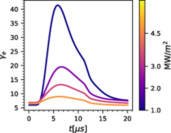
Figure 14. The sheath heat transmission coefficient during perturbations launched on several different initial input power backgrounds - kinetic perturbation on kinetic background.
Download figure:
Standard image High-resolution image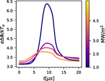
Figure 15. The sheath potential drop during perturbations launched on several different initial input power backgrounds - kinetic perturbation on kinetic background.
Download figure:
Standard image High-resolution imageIn order to evaluate the differences between kinetic perturbations launched on fluid and kinetic backgrounds, the following quantity is plotted in figure 16

where y is either γe or eΔΦ/(kTe), while KK and FK denote values during the kinetic perturbation on the kinetic and fluid backgrounds, respectively. In general, the fluid background cases underestimate the two quantities, and the 'error' grows as input power is increased, except for γe, where it seems to follow the rollover behaviour from figure 8 and drops after 3MW m−2. δ for both quantities is most pronounced in the first ≈ 2 µs of the perturbation, with secondary peaks after ≈ 4 µs for γe. Values of δ between 7 − 10 µs show that the relative errors of the peak values of γe and eΔΦ/(kTe) are below 25% and 5%, respectively, with the peak error of γe for the lowest input power less than 5%. The largest γe error here is observed for the input power of 3MW m−2, when the rollover in the sheath heat transmission coefficient happens. The large deviation at 3MW m−2 is likely caused by the fact that the fluid and kinetic backgrounds differ qualitatively, as the fluid background is attached, while the kinetic model predicts detachment at this power.

Figure 16. The relative deviation of the two sheath properties when the kinetic perturbation is launched on the kinetic versus fluid backgrounds.
Download figure:
Standard image High-resolution image
5. Discussion
We begin the discussion of the presented results by going over the main limitations of the present study inherent to the model used, as well as limitations of scope. The first major assumption is that of dimensionality, as we use a 1D model. However, for the study of kinetic effects in the SOL, especially as they relate to equivalent fluid scenarios, we expect this study to be able to capture the differences due to those kinetic effects.
Two limitations we plan to tackle in a future version of the SOL-KiT code are the  approximation, as well as the limited neutral physics (currently only diffusive-reactive atoms included, with elastic electron-neutral collisions ignored). These two primarily limit the parameter space accessible to us, and the fundamental aspects of the results presented in this study should not be greatly affected by them, especially since the study is based on comparing two models which use the same approximations. However, future work is being planned to investigate this rigorously.
Use of harmonics only up to l = 1 is another simplification in the current study. While this approximation captures most of the physics, simulations using it will naturally underresolve kinetic effects, as the allowed anisotropy of the distribution function is limited. Furthermore, we expect the greatest impact of including higher l terms to be at the boundary, where a better angular resolution in velocity space allows for higher accuracy in the sheath boundary condition. Exploring higher harmonic effects will be the topic of a future study, as SOL-KiT has all of the necessary features, with the only constraint being the computational time required to obtain kinetic equilibria with a high level of anisotropy. Preliminary results with higher harmonics confirm that they tend to be localized near the boundary, and that the error in taking lmax = 1, while present, is not prohibitive, with relatively weak effects on profiles. Quantifying the role of anisotropy in simulations like those presented here, and stress-testing cases with anisotropic sources will be the topic of a future work.
Magnetic effects are not included in the present study, and the addition of magnetic mirroring and curvature effects will surely increase the anisotropy of the distribution function. This would be an interesting avenue for future research. Finally, the sheath model used in this study, together with our treatment of the electric field and the geometry of the problem, does not include potentially interesting effects such as those arising from currents during transients [31] or due to subsonic sheaths [32]. In order to add a constant current in our 1D model, a modification to our E field equation would be necessary, effectively mimicking a  term. It is not clear whether these effects would be strong in the scenarios we have studied here, but improvements to the field and sheath models are likely candidates for an upgraded version of the current code.
We have presented in this study both equilibrium and transient simulations of parallel electron transport in the SOL, treating the electrons as either a fluid or kinetically. The equilibrium results (for the parameters in this study), while showing the presence of kinetic effects, do not appear to be dominated by them. We report the rollover of the plasma flux into the target sheath, which is interpreted as the onset of detachment. The input power at which this occurs is different for the fluid and kinetic models, with the rollover happening at a lower input power when electrons are treated as a fluid. Rollover at a lower power in the fluid case can be explained by the fact that temperatures near the target are greater compared to the kinetic model, leading to a higher degree of ionization. The equilibrum kinetic effects, which occur as heat flux enhancement and suppression, depend heavily on the spatial location and the input power. This makes it difficult to prescribe one (or even a set) of flux limiters that could capture the physics, especially the flux enhancement. We also report on the fraction of heat flux carried by fast tail electrons near the target in table 1. It is found that it is non-negligible even for the lowest power equilibria. Another equilibrium kinetic effect that has been explored here is the modification of the electron sheath heat transmission coefficient, where we find up to ≈ 40% variation with respect to the assumed classical fluid value of γe≈ 5. The values of γe agree well with the highly radiative JET case explored in the literature using KIPP [11], while the qualitative non-monotonic behaviour ("rollover") in the heat transmission coefficient agrees with both KIPP [11] and BIT1 results [5].
While a clear dominance of kinetic effects was not found for the equilibrium simulations, runs with short conductive transients provide a different picture. Firstly, the target temperature during the perturbation predicted by the fluid model is approximately two times higher than when electrons are treated kinetically (figure 10). One could imagine imposing a flux limiter in the fluid case to mimic this, but we present results showing vastly different evolution of the conductive electron heat flux (with respect to its classical value) for both different spatial points in the system, as well as different initial input powers (see figures 11 and 12). For example, the ratio close to the target reaches values of up to 10 during the short perturbation studied here, before quickly dropping down below 1. With a mix of heat flux suppression and enhancement, as well as their time-dependent nature, it is highly unlikely that a simple modification to the flux could reproduce the full range of behaviours simulated here. However, it might be worthwhile to explore more complicated fluid models for capturing kinetic effects (see, for example, Brodrick et al [33]), and compare them to the results obtained in this study. Reduced gyrokinetic moment-based approaches could also be a fertile ground for cross-model comparisons [34]. We also present the variation of the sheath heat transmission coefficient, as well as the sheath potential drop, during the perturbation. Both show significant modification compared to their classical values, with the maximum deviations from classical values being up to 8 times for γe and more than 2 times for eΔΦ/(kTe). This indicates a likely need to include time-dependent models for the sheath behaviour during transients simulated using fluid codes, as argued also by Havlíčková et al [13]. While not treated in this study, it is likely that kinetic effects will compound in repeated perturbations of the kind treated here (loosely corresponding to type III ELMs [7]). A more detailed kinetic study of this scenario is certainly required.
It is worth repeating that all of the presented perturbation simulations were performed in the same way, increasing the input power to the same value (45MW m−2) for the same amount of time (approximately 10 µs). However, the intensity of kinetic effects varied strongly as a function of initial conditions, namely the initial input power of the used equilibrum profiles. This suggests, as one might expect, that the degree of kinetic modification to the physics depends on the ratio of the initial input power to that of perturbation. Further investigation is required to explore this facet of the simulations, with a special focus on the way energy is injected into the system, and this will be presented in a separate publication.
Finally, we explored the approach of launching kinetic perturbations on fluid equilibria. While there are discrepancies due to the fluid equilibrium relaxing (see figure 16), the perturbation behaviour is well captured using this approximate method, especially that of the sheath potential drop, where discrepancies quickly drop below 5%. As the equilibria are reached on fluid timescales, the fact that the kinetic model requires a much shorter timestep increases simulation times. Since the computational time saved when using a fluid equilibrium as the base for kinetic transient studies is considerable (an order of magnitude longer times for kinetic equilibria), having the option of performing quick simulations to explore qualitative aspects of the perturbation behaviour is encouraging.
Given the above results, one can infer the sorts of effects that would be needed in a reduced fluid model of the SOL if kinetic effects are to be included. While simple solutions like flux limiters are likely insufficient, an iterative coupling approach is currently being investigated with SOL-KiT, where corrections from the kinetic model are fed into the fluid model directly. This has the effect of speeding up kinetic equilibrium calculations by an order of magnitude, making their computation time comparable to pure fluid mode calculations, and will be introduced in a future publication. However, if such an approach is not an option, one would have to consider both heat flux effects (possibly using an input power dependent flux limiter based on spatially averaged kinetic results), as well as kinetic modifications to boundary conditions (especially γe). Nonetheless, due to the more pronounced kinetic effects in transients, it would seem that more detailed kinetic models are necessary.
The parameter ranges of the presented results are mostly relevant to MSTs, specifically to the interaction of transients with detachment in such machines. In larger machines, we expect that for similar collisionalities to those treated here the kinetic effects would manifest in a qualitatively similar manner. This would require a corresponding scaling up of the input power and density in order to compensate for an increase in connection length. As our simulations require resolving the collision times, denser plasmas would be much more computationally expensive, but studies of this form have been planned.
6. Conclusion
We presented the first study of parallel electron transport using the newly developed fully implicit code SOL-KiT. Both equilibria and transients were simulated, using the capability of the code to simulate electrons as a fluid or kinetically, with the two models being consistent with each other. The parameters used in these simulations are mostly relevant to medium sized tokamaks.
For equilibria, kinetic effects are not dominant, but they still change the behaviour compared to that obtained in equivalent fluid runs. In particular, we report detachment onset at different input powers for different electron models, with detachment surviving up to a higher input power in the kinetic case. Also, a variation of the electron sheath heat transmission coefficient of up 40% compared to the classical value of ≈ 5 is observed.
Significant kinetic effects were found during transients, especially in the transport properties of the target sheath, where it was found that the electron sheath heat transmission coefficient could reach up to 8 times its classical value, with the sheath potential drop reaching values greater than 6kTe/e. We compare simulations using different initial conditions as well as different models for the electrons (fluid or kinetic), and find both heat flux suppression and enhancement in both equilibrium and transient simulations. The fluid model is found to systematically overestimate the temperature at the target due to a lack of heat flux suppression. A considerable amount of sensitivity to initial conditions was observed in transient simulations, with different backgrounds experiencing greatly varying levels of kinetic effects.
We show that an accurate prediction of the evolution of heat flux during transients in the SOL requires a kinetic approach to modelling electrons, as the variable transport quantities during transients would be extremely difficult to simulate using flux limiters.
Acknowledgment
This work was supported through the Imperial President's PhD Scholarship scheme. This work was partially funded by the RCUK Energy Programme [grant number: EP/T012250/1]. Simulation results were obtained with the use of the Imperial College Research Computing Service [35]. We would also like to thank the two anonymous reviewers for their contributions in improving this paper.
Appendix: On the consistency between the fluid and kinetic models of SOL-KiT
Since the study presented here focuses on the comparison between a fluid and a kinetic treatment of the electrons, and relies heavily on the consistency between the two treatments, it is worth addressing this topic in more depth. As noted in the main text, by consistency we mean that the two models are using the same atomic data, as well as the fact that the fluid model is obtained by taking the appropriate moments of the kinetic equation and applying classical closures. In this appendix the explicit form of the moments for each transport quantity is presented, and the classical closures are contrasted with the corresponding kinetic expressions.
It is useful to define a shorthand for the nth scalar moment of fl
Using equation (A1) all of the usual moments can be defined following standard Legendre harmonic procedures from the literature [23]. These are


where Ue is the electron internal energy density,  the total, while qe is the conductive heat flux. Pii (i = 1, 2, 3) are the diagonal components of the pressure tensor, with the off-diagonal components zero due to symmetry. Since the presented results here are obtained with harmonics up to l = 1, f2 = 0, and the pressure tensor reduces to just
  .
.
A relatively simple way to derive the fluid equations used in SOL-KiT is to follow standard moment taking procedures starting with equation (10) (instead of (12)). Once the conservative forms of the fluid equations are obtained, any approximations arising from the harmonic expansion can be added following the above moment definitions (for example, the pressure can be set to isotropic if the l = 2 harmonic is not present). For completeness, the conservative forms of the parallel momentum and energy equations (equations (2) and (3)) are
The pressure tensor in the above equations uses a simplified form, due to f2 = 0. However, one could put in the Braginskii [2] closure for the tensor, if performing fluid-kinetic comparisons with a higher number of harmonics.
In order to calculate the sources and sinks, excitation and ionization rates are calculated in the following way, as noted in the main text
where σTOT is the integral cross-section for the given process taken from Janev [18] (with inverse process treated using the principle of detailed balance). In this way, f0 can be replaced by a Maxwellian and the same terms can be used in the fluid model. This is one of the key elements in our claim of consistency - the use of the same cross-section data between the two models, with only the distribution functions being different. The particle source/sink term in the fluid model is then
The inelastic collision contribution to the heating term  in equation (3) is
where the sum is over all atomic states (including the ionized state), and is a shorthand for all of the relevant collisional processes in equation (7).  represents the transition energy associated with a particular process (e.g. ionization or excitation energy). Finally, the electron-neutral friction in the fluid model is calculated using terms of the following form
where  (with Maxwellian f0), and the integrand in this case is equation (28). The particular form of f1 corresponds to a slowly (compared to the electron thermal speed) drifting Maxwellian [23]. Given that the flow is on the scale of the ion sound speed, it is
  times smaller than the electron thermal speed.
Besides the above closures associated with atomic processes, there are the classical closures of the conductive heat flux qe, electron-ion friction Rei, and the sheath heat transmission coefficient γe. As noted in the above text these are taken from the literature [2, 17], and are presented again in table A1 along with their kinetic counterparts to clarify the differences between the fluid and kinetic models. The first row of the table shows the conductive heat flux, with the Braginskii value taken for the fluid closure, and the isotropic pressure value taken for calculating the kinetic convective heat flux. Since  , the Braginskii value reduces to just the temperature gradient (Spitzer-Härm) contribution. A popular way to generalize this closure to account for domains of the simulations which are not truly collisional is to introduce a flux limiting factor (flux limiter) α, writing the heat flux as [3]
where qT is the classical value, and  is some fraction α of the free streaming flux. The study presented here essentially interrogates the validity of this approach.
Table A1. Fluid closures due to non-atomic processes and their kinetic counterparts in the SOL-KiT model. The integrand in the friction term is the electron-ion collision operator.
| Fluid | Kinetic | |||
|---|---|---|---|---|
| qe |  |
 |
||
| Rei |  |
 |
||
| γe |  |
 |
In a similar way to the heat flux above, the fluid friction reduces to the thermal force. The kinetic value for the friction would be given by the first moment of the electron-ion collision integral. Finally, the last row of the table shows that the electron heat transmission coefficient is calculated using the cut-off distribution at the sheath, following the definition in equation (9).
There are fundamentally only two groups of quantities that differ between the kinetic model and its fluid reduction used in the code. The first group is the atomic sinks/sources of particles and energy, as well as electron-neutral friction. Since both the kinetic and the fluid model use the same cross-sections in calculating these quantities, the only differences come from the electron distribution function, with it being a slowly drifting Maxwellian in the fluid model. The second group is the classical closures, where the fluid model takes widely used expressions. It should also be noted that both models are embedded in the same numerical framework. In this way, the SOL-KiT framework allows for the identification of kinetic effects in electron transport without the potentially confounding consequences of using a fluid model that is not consistent with the kinetic electron model.