

Abstract
A simple model for the instrument function of scintillator-based fast-ion loss detectors (FILD) has been developed which accounts for the orbit trajectories in the 3D detector geometry and for the scintillator response. It allows us to produce synthetic FILD signals for a direct comparison between experiments and simulations. The model uses a weight function formalism to relate the velocity-space distribution of fast-ion losses reaching the detector pinhole to the scintillator pattern obtained experimentally, which can be understood as a distortion of the velocity-space distribution due to the finite resolution of the system. The tool allows us to recover the undistorted velocity-space distribution of the absolute flux of fast-ion losses reaching the detector pinhole from an experimental measurement using tomographic inversion methods, which can reveal additional details of the velocity-space distribution of the lost ions.
Export citation and abstract BibTeX RIS
1. introduction
It is well known that in magnetically confined fusion plasmas, fast (suprathermal) ions play an important role in key aspects such as plasma heating efficiency, magnetohydrodynamic (MHD) stability and current drive [1, 2]. Moreover, the confinement of the fast-ion population is crucial for the optimal operation of fusion devices, since, if sufficiently localized and intense, fast-ion losses may lead to irreversible damage to the plasma-facing components [3]. Comprehensive knowledge of the fast-ion distribution and the mechanisms leading to a deterioration of the fast-ion confinement is therefore required. In this sense, fast-ion loss detectors (FILD) [4–8] have been proved to be an excellent tool to investigate the underlying mechanisms leading to enhanced fast-ion losses induced by MHD fluctuations [3, 9–12], edge localized modes [13] or externally applied 3D magnetic perturbations [13–15].
Scintillator-based FILDs consist of a scintillator plate mounted in a probe which is placed near the plasma, in the far scrape-off layer. The escaping fast ions reach a pinhole in the probe head and go through a 3D collimator that filters the ion trajectories. This allows a direct measurement of the Larmor radius and pitch angle of the fast ions. A more detailed description of the FILD detector can be found in [6]. FILD detectors provide valuable information about the temporal evolution of the velocity-space of the fast-ion losses. However, the interpretation of the FILD signals is not always straightforward. The finite size of the collimator limits the resolution of the detector in pitch angle and Larmor radius. The distribution measured on the scintillator plate can be thought of as a distortion of the velocity-space of the losses reaching the detector pinhole due to the limited resolution. Although previous work has reported on some aspects of the resolution limitations of FILD diagnostics [4, 10, 16–18], a comprehensive description of the velocity-space sensitivity of the detector is given here for the first time. A simple model based on a weight function formalism is presented which allows us to relate the fast-ion flux reaching the detector head to the pattern measured by the scintillator. These weight functions are analogous to those used for confined fast-ion diagnostics [19–25]. The weight functions allow us to write the forward model of the diagnostic response as a matrix equation that can be solved by tomography in velocity-space [26–31].
The paper is organized as follows: first, a description of the trajectory calculations in the FILD head is provided; second, the model that describes the detector response is presented; third, the application of velocity-space tomography to the FILD signal is presented with a sensitivity study and experimental benchmark; finally, conclusions are discussed.
2. Orbit calculations
In order to characterize the response of the FILD detector, trajectory calculations of the ions are carried out with the FILDSIM code. The code computes the ion trajectories started in the entry plane of the detector pinhole and follows them on their way up to the scintillator. It detects any collisions between the ions and the realistic 3D detector geometry elements. The code assumes that the local magnetic field in the volume of the head probe is constant. In the majority of the devices, this assumption is justified given that the size of the FILD probe head, typically determined by the size of the gyroradii of the ions that we want to measure, is small compared to the size in which the magnetic field variations are relevant. For example, in medium size tokamaks such as ASDEX Upgrade, the magnetic field variation in such a volume is found to be of the order of <1%. Therefore, there is no need to solve the Lorentz equation of motion since the analytical solution of the ion orbits in a constant magnetic field are well known to be helixes. Figure 1 shows qualitatively how the probe head looks like and how the trajectories go through the collimator and hit the scintillator. The dimensions of the ASDEX Upgrade FILD1 elements are indicated in table 1 for reference.

Figure 1. (a) 3D view of a typical FILD probe head (dark gray) and the scintillator (green). Fast-ion orbits are shown in red (blocked by the collimator) and blue (not blocked by the collimator). The strike map (in white) is overlayed on the scintillator. (b) and (c) show more detailed side views of the collimator highlighting the most important parameters.
Download figure:
Standard image High-resolution imageTable 1. Dimensions of the main elements shown in figure 1 corresponding to the particular case of FILD1 at ASDEX Upgrade.
| Geometry element | Dimensions |
|---|---|
| Pinhole length | 2 mm |
| Pinhole width | 0.5 mm |
| Slit height | 10 mm |
| Pinhole—scintillator distance | 5.75 mm |
| Probe head diameter | 7.2 cm |
| Scintillator dimensions | 3.3 × 4.8 cm2 |
A number N of ions with fixed gyroradius and pitch angle are started with random positions in the entry plane of the pinhole and random gyrophases. The ions are followed until they collide with the scintillator or with any other geometry element. This process is repeated for the relevant range of gyroradius and pitch angle values. It should be noticed that throughout this paper we will refer to the ion gyroradii rather than their energies. This is because the FILD diagnostic measures the Larmor radius of the particles regardless of what species the particle is. Given the magnetic field at the probe position, the energy can be calculated for any impinging ion species. The information that can be retrieved from this simulations is described in the following.
Ion trajectories started at the pinhole with a fixed value of gyroradius and pitch angle have a distribution of strike-points in the scintillator due to the random initial positions and gyrophases of the ions. The centroid of such a distribution can be computed for all gyroradius and pitch angle values leading to a strike map, an example of which is shown in white in figure 1(a). This strike map defines the velocity-space of the ions measured in the scintillator, given by the gyroradius  and the pitch angle Λ'.
The size and shape of these distributions give information about the resolution of the detector. The resolution in gyroradius is illustrated in figure 2(a), which shows the gyroradius distribution profiles obtained in the scintillator velocity-space ( ) along a line of constant pitch angle (Λ'). The different colors correspond to different values of the particle gyroradius started at the detector pinhole. The strike-point distributions can be fairly well modeled as asymmetric Gaussian (skew Gaussian). The fit to this model is represented by the solid lines in figure 2(a). It can be seen that for small values of the ion gyroradius, the distributions do not overlap, and thus different spots in the scintillator can be easily identified. However, if two strike-point distributions for different values of gyroradius and pitch angle overlap, no direct one-to-one mapping between the velocity-space in the pinhole and the velocity-space on the scintillator exists, and this is what happens for larger gyroradii values. Figure 2(b) shows one of these strike-point distributions in detail. It can be observed that the strike-points distribution fits better to a skew Gaussian function (red curve) than to a Gaussian function (black curve).
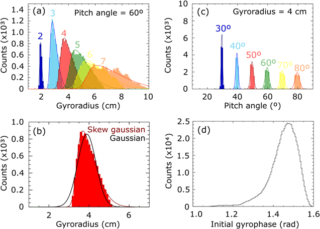
Figure 2. (a) Gyroradius distribution profiles in the scintillator velocity-space along a line of constant pitch angle. Different colors correspond to different values of the particle gyroradii started at the FILD pinhole. The solid lines are the fit to the skew Gaussian model. (b) Zoom into a single distribution. The fit to a Gaussian distribution is shown in black, while the fit to a skew Gaussian function is shown in red. (c) Pitch angle distribution profiles in the scintillator velocity-space along a line of constant gyroradius. Different colors correspond to different values of the particle pitch angle started at the FILD pinhole. The solid lines are the fit to the Gaussian model. (d) Histogram of the particles initial gyrophase which are not blocked by the detector collimator.
Download figure:
Standard image High-resolution imageOn the other hand, the resolution in pitch angle is illustrated in figure 2(c), which shows the pitch angle distribution profiles obtained in the scintillator velocity-space (Λ') along a line of constant gyroradius ( ). In this case, the strike-point distributions are modeled by Gaussian functions. A similar resolution is obtained for all pitch angle values.
Some of the markers started at the pinhole will not impinge on the scintillator but will be blocked by the collimator. We define the collimator factor as the ratio between the number of markers reaching the scintillator and the number of markers started at the pinhole,  , for fixed values of gyroradius and pitch angle. The collimator factor is needed, for instance, to estimate the absolute flux of fast-ion losses at the FILD probe head. The ions that are not blocked by the collimator are those whose initial gyrophase lies inside an acceptance cone, which is determined by the collimator geometry (figure 2(d)).
The properties described above are determined by the design of the collimator, whose main parameters are illustrated in figures 1(b) and (c). For instance, a wider pinhole or a wider slit will generally lead to a larger collimator factor (this is, a smaller fraction of the incoming ions being blocked) at a cost of lower resolution in gyroradius, which will be described later. The resolution in pitch angle is mainly determined by the length of the pinhole, while the height and the angle of the slit determine the range in velocity-space that can be measured. A compromise between these properties must be made when designing the collimator.
3. FILDSIM model
With the information obtained in the trajectory simulations we propose a simple model to relate the velocity-space of the ions reaching the FILD pinhole  , to the pattern measured by the scintillator
  , which can be understood as a distortion of the velocity-space of the losses in the pinhole due to the finite resolution of the system. Notice that the' is used to differentiate between the velocity-space defined at the pinhole and the velocity-space defined at the scintillator. Using a weight function formalism similarly to what is done in other fast-ion diagnostics such as FIDA, CTS or NPA [19–25, 32, 33], the signal measured at the scintillator can be expressed as:
ΓS is the measured signal in the gyroradius range  and pitch angle range
  in units of (photons), which depends on the velocity-space coordinates defined in the scintillator. ΓP is the velocity-space distribution of the lost ions in the pinhole in units of
  , and w is the instrument weight function, thus in units of
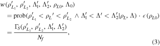
  . The weight function in this case can be split into the product of a probability function prob
  , which maps the distribution in the pinhole to the distribution measured in the scintillator, and a function accounting for the yield of the scintillator
  (ρL) which is described later. The probability function can then be thought of as the probability that an ion reaching the pinhole with gyroradius ρL and pitch angle Λ has to impact the scintillator in a region such that
  and
and  .
.
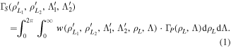
Formally the weight function  can be calculated evaluating the expected pattern in the scintillator by introducing a δ-function in equation (1) in place of the velocity-space distribution of the ions reaching the pinhole ΓP:

where Nf is the number of ions with a certain gyroradius  and pitch angle Λ0. This is what we effectively do in the trajectory simulations described in the previous section. The amplitude of the weight function at the velocity-space position ρL0, Λ0 is then:
where  is the scintillator efficiency. The efficiency function contains the information about the yield of the scintillator, this is, the number of photons emitted by the scintillator per incident ion, which is a function of the particle species and energy. The characterization of the scintillator material (TG-Green in this case) [34, 35] has been carried out in an accelerator facility. Figure 3 shows the experimental measurements of the scintillator yield as a function of energy for protons, deuterium and alpha particles. A good agreement is observed with the theoretical values obtained from the application of the Birk's model [34]:

where  is the photon yield per unit length,
  is the stopping power of the incident particles, and S and k are constants inferred from the measurements which are related to the scintillator efficiency and the degree of quenching, respectively. This model is used to obtain the scintillator yield at lower energies, of interest for NBI generated fast ions.

Figure 3. Yield of Tg-Green scintillator for the different species of interest. Full lines correspond to the experimental measurements, while dashed lines correspond to the theoretical values obtained from Birk's model.
Download figure:
Standard image High-resolution imageBy discretizing the velocity-space, equation (1) can be expressed in matrix form as:

where the separation between the probability function, labeled as T, and the scintillator efficiency function is explicitely highlighted.
In principle the probability matrix can be calculated numerically from the trajectory calculations. However, the velocity-space of the FILD signals is typically discretized with Δρ ∼ 0.1 cm and ΔΛ ∼ 1°, so that the details of the distribution can be resolved. This usually leads to a matrix size for ΓP of 100 × 90 elements, which means that orbit trajectory calculations should be done for 9000 pairs of gyroradius and pitch angle values. In order to get good statistics typically 105 markers are simulated for each pair. To save computational time and as a useful tool to gain insight quickly, we develop an analytical model for the shape of the probability functions. As it has been shown in the previous section in figures 2(a) and (c), the projections of Tij for a fixed k and l can be modeled as skewed Gaussians. Using this approximation the elements of the probability matrix Tijkl can be written as:
where fcol is the collimator factor, σρ and σΛ are the parameters controlling the width of the distribution, erf is the error function and αρ is the parameter controlling the skewness of the distribution in the gyroradius direction.
Figure 4 shows the comparison between a 2D distribution obtained directly from the orbit calculations (a) and the fit to the analytical model (b), where the distributions have been normalized to unity. Slight differences can be observed as shown in figure 4(c). The main discrepancy is of the order of ∼15% and is obtained in the edges of the distribution. This is due to the tails of the Gaussian functions, which do not fall to zero as sharply as the simulated distributions. However, in general terms a good agreement is found between the fitted model and the results obtained from the orbit calculations.

Figure 4. (a) 2D histogram of the strike-points obtained from the orbit calculations in the gyroradius-pitch angle space at the scintillator. (b) 2D histogram obtained from the fitted analytical model. (c) Difference between (a) and (b). Overall, a good agreement is found between both. The main discrepancies are observed in the edges of the distribution, due to the tails of the Gaussian functions, which do not fall to zero as sharply as the simulated distributions.
Download figure:
Standard image High-resolution imageThis way, it is possible to perform the orbit trajectory calculations on a much coarser grid (i.e. 10 × 9), and build a finer grid by interpolation of the parameters in the model fcol, σρ, σΛ and α, which are functions of the velocity-space coordinates ρ and Λ defined in the pinhole and behave well in terms of continuity and differentiability, as shown in figure 5. It can be seen that the collimator factor ranges from 0% to 4%. The resolution in gyroradius, approximated by σρ, becomes lower for larger gyroradii as was previously described, while the resolution in pitch angle is similar throughout the whole velocity-space being approximately ∼1°, although a slight dependence with the pitch angle is observed.

Figure 5. Contour plots of the main parameters of the model, defined in the pinhole space ρ − Λ. (a) σρ, (b) σΛ and (c) fcol.
Download figure:
Standard image High-resolution imageThe behavior of the FILD weight function is schematically illustrated in figure 6. In figure 6(a), different positions in the pinhole velocity-space are represented by the empty diamonds. Associated to each of these points, isolines of the strike-point distribution in the scintillator are represented by the solid lines. All of these lines go through the same point in the scintillator velocity-space, represented by a black cross. Correspondingly, in figure 6(b) the dashed lines represent contour levels in the pinhole velocity-space which would lead to the same signal per ion at the mentioned position in the scintillator velocity-space. The blue line corresponds to a larger probability than the green line.

Figure 6. Cartoon illustrating the behavior of the FILD weight function. (a) Shows the isolines of strike-points in the scintillator for different points in the pinhole. (b) Shows the isolines of points in the pinhole leading to the same signal per ion in the scintillator. (c)–(e) illustrate the FILD weight function showing the region of the velocity-space in the pinhole (contour) that can produce signal in a certain point of the velocity-space in the scintillator (black cross).
Download figure:
Standard image High-resolution imageFigures 6(c)–(e) show the FILD weight functions for a fixed pixel of the scintillator velocity-space. It shows the regions of the velocity-space in the pinhole k, l (contour plot) which generate measurable signal in the scintillator velocity-space bin i, j (black cross). The black regions do not generate any signal in that velocity-space bin. It can be noticed that the weight functions are well localized in the pitch angle direction, while they are rather extended in the gyroradius direction and not symmetrical with respect to the scintillator velocity-space bin. This can be understood by looking at the skewed Gaussian distributions discussed in section 2, which are wider for larger gyroradii. It is therefore more likely for a bin in the scintillator velocity-space to pick up signal from large gyroradii regions in the pinhole velocity-space rather than from low gyroradii regions.
Using equation (5), it is straightforward to obtain the velocity-space distribution at the scintillator given a velocity-space distribution of the losses at the FILD head probe. The latter can be provided by orbit following codes such as ASCOT [36] or OFMC [37]. This is of great utility to compare the experimental measurements with simulations [3]. Otherwise, the direct comparison can sometimes be misleading, in particular due to the limited resolution of the system at large gyroradii.
For comprehensive comparisons with the codes, the raw measurements need to be related to the velocity distribution on the scintillator plate. This is possible provided a full characterization of the scintillator response and a calibration of the optical system [35]. The velocity distribution on the scintillator is obtained from the raw signal as follows:

where  is the raw measurement, this is, the counts measured for each pixel p, q of the camera frame, Cpq is a calibration matrix, and Rijpq is a matrix which maps the frame pixels to the velocity-space coordinates.
The calibration matrix Cpq contains the information about the full calibration of the optical system, which consists basically of a set of lenses, a beam splitter and a bandpass filter. The calibration is performed using an intengrating sphere which provides a well known integrated photon flux. This light source is placed in the scintillator position and a calibration frame is recorded with the data acquisition system, in this case a camera. The calibration matrix takes the following form:

where ΦIS is the photon flux provided by the integrating sphere, SΩ is the area of the integrating sphere that a pixel of the camera is effectively viewing, ΔtIS is the exposure time of the camera for the calibration frame, AP is the area of the pinhole, Δt is the camera exposure time, and IISpq is the number of counts in each pixel for the calibration frame. By including the absolute calibration of the detector in this model we overcome two previous limitations: on the one hand, the tomographic inversion can be applied to arbitrarily complex velocity-space distributions without the need to define any region of interest. On the other, this approach now takes into account implicitly the finite resolution of the system.
The inverse problem is also of interest: given a measurement of the velocity-space distribution in the scintillator ΓS, we would like to retrieve the undistorted velocity-space distribution of the absolute flux of fast-ion losses reaching the FILD head probe ΓP, which is the physically relevant information. Combining the matrices from equation (7) we recover the matrix equation:

where the unknown is the velocity distribution of the fast-ion flux at the pinhole  , whereas the other two quantities are known: the absolutely calibrated velocity-space distribution measured at the scintillator
  and the weight function Wijkl, which is a combination of the probability function and the efficiency function. The solution for
  in equation (9) is mathematically an ill-posed problem, analogous to the problem faced by velocity-space tomography for other fast-ion diagnostics [26–31]. Therefore, the same inversion techniques can be used to solve it such as those described in [29]. In particular, the 0th order Tikhonov regularization method has been implemented. In general, the Tikhonov regularization methods solve a minimization problem which can be expressed as:
where W is a matrix composed of weight functions, S is the measurement matrix and F is the solution we seek. The upper row minimizes the two-norm residual of S = WF, while the lower row penalizes large values of the two-norm of λLF. The definition of the L matrix can then be done based on the properties of the solution F that we want to penalize. The regularization parameter λ controls the balance between the strength of the regularization condition and the goodness-of-fit to the data. Therefore, an optimal value for λ must be found. Different choices of the L matrix give name to the different Tikhonov methods. In 0th order Tikhonov regularization method large absolute values of the solution F are penalized by choosing L = I, the identity matrix. Additionally, adding a non-negativity constraint to the regularization method [30] showed to improve the results of the inversion. The non-negativity constraint is trivially justified, since we know that the velocity-space distribution is not negative. Some examples are shown in the following section.
4. Sensitivity study of the FILD tomography
The method described in the previous section has the potential to counteract the distortion of the velocity-space in the detector, which can help the interpretation of the measurements. In order to assess the capabilities and limits of the technique, we have carried out a sensitivity study by performing tomographic inversions to synthetic FILD data under different conditions.
For this study we will use a synthetic pinhole distribution consisting of three different monoenergetic distributions at ρL = 3.1 , ρL = 4.3 and ρL = 5.4 cm with a certain spread in pitch angle. This is shown in figure 7(a). Such a distribution mimics typical FILD data expected at AUG for the detection of first orbit NBI losses corresponding to the three energy components. As it was mentioned in section 3 we will use the 0th order Tikhonov regularization method with non-negativity constraint for the inversion.

Figure 7. (a) Synthetic pinhole distribution used for the sensitivity study of the tomography. (b) Synthetic scintillator signal without noise. (c) Recovered pinhole distribution after applying the tomographic inversion.
Download figure:
Standard image High-resolution imageAs a proof-of-principle, we first generate the synthetic FILD signal under idealized conditions, this is, without noise. The result is shown in figure 7(b), where the expected synthetic signal in the scintillator is shown. It can be observed how the finite resolution of the instrument function smears out the signals corresponding to each of the different gyroradius components. It is also noticeable how the resolution in gyroradius becomes worse for larger gyroradii: the spot corresponding to ρL = 3.1 cm is clearly distinguishable, while the components ρL = 4.3 and ρL = 5.4 cm are not discernible and produce a single spot. After applying the tomographic inversion we are able to recover the undistorted velocity-space at the pinhole, shown in figure 7(c). This proof-of principle test reveals the potential of the tomographic inversion technique to improve the energy resolution of the FILD measurements. However, the almost exact resemblance of the true solution and the inversion is only achieved in this idealized situation without noise.
We are now interested in evaluating the behavior of the technique in a realistic case when considering noise in the signal. In FILD we can define the signal-to-noise ratio as  , where Imax is the maximum signal of a pixel in the measurement, and
  is the mean noise level. The latter is obtained from camera frames in the absence of fast-ion signal. The intensity of the pixels is found to follow a Gaussian distribution, from which the mean value is obtained.
Taking into account the dynamic range of the cameras used in the AUG FILD systems, the maximum SNR achievable, which would correspond to the case in which the center of the measured spot saturates, is in the order of SNR ∼ 200. Attending to this estimate, we can add different noise levels to the synthetic FILD signal and evaluate the tomographic inversions. This is shown in figure 8, where the tomographic inversions for different noise levels corresponding to SNR = 200, 100 and 20 are shown. As the noise level is increased, the quality of the recovered pinhole distribution is lowered. However, in any case the three different gyroradius distributions can be qualitatively observed in all the cases. It should be mentioned that in all of these inversions the selection of the optimal regularization parameter λ has been done through the L-curve method [29].

Figure 8. Synthetic scintillator signals with different noise levels (a) SNR = 200, (b) SNR = 100, (c) SNR = 20, and their tomographic inversion in (d)–(f) respectively.
Download figure:
Standard image High-resolution imageIt is also of interest to evaluate if the inversion is able to distinguish between energy spread distributions and monoenergetic components. This is motivated by the fact that NBI first orbit losses are routinely measured by the FILD systems, which by definition are expected to be measured as monoenergetic distributions with energies corresponding to the NBI injection systems, without any loss of energy. To investigate this we perform several simulations in which we change the spot at ρL = 5.4 cm and increase its spread in energy, assuming deuterium ions and a local magnetic field of BFILD = 1.4 T. Figures 9(a)–(c) show the different synthetic pinhole distributions used for this scan, corresponding to energy spreads of σe = 10 keV, σe = 20 keV and σe = 50 keV respectively, keeping the same total amount of ions. Figures 9(d)–(f) show the corresponding synthetic scintillator signal, with a noise level such that SNR = 200. The differences between them are barely noticeable. The results of the tomographic inversion are shown in figures 9(g)–(i). It is observed that the tomography is in fact able to distinguish between the two cases. However, as the energy spread is increased, the inverted distribution loses its capability to localize the individual peaks in energy and the retrieved distribution is smoothened out.

Figure 9. Sensitivity scan in which the energy spread has been increased only for the spot centered at ρL = 5.4 cm. (a)–(c) Synthetic pinhole distribution. (d)–(f) Synthetic scintillator signal. (g)–(i) Tomographic inversions. (a), (d), (g) correspond to σe = 10 keV, (b), (e), (h) correspond to σe = 20 keV, and (c), (f), (i) correspond to σe = 50 keV, assuming deuterium ions and a local magnetic field of BFILD = 1.4 T.
Download figure:
Standard image High-resolution imageThe last check consists of evaluating the energy resolution of the tomography, this is, the capability of the technique to disentangle different monoenergetic distributions. In order to do this we take the distribution at ρL = 5.4 cm and move it closer to the distribution at ρL = 4.3 cm. A scan has been performed by positioning the distribution at ρL = 4.5–4.8 cm, illustrated in figures 10(a)–(c). The corresponding synthetic scintillator signals are shown in figures 10(d)–(f), where again the differences are barely perceptible. Figures 10(g)–(i) show the results of the tomographic inversions. It can be observed that there is a limit in the gyroradius of the distribution that the tomography is able to disentangle. This limit depends on the SNR of the particular case and on the gyroradii of the distributions that we want to disentangle. Smaller values of the SNR and larger values of the gyroradii of the distributions, will make it more difficult for the tomography to disentangle them.

Figure 10. Sensitivity scan varying the gyroradius separation between spots. (a)–(c) Synthetic pinhole distribution. (d)–(f) Synthetic scintillator signal. (g)–(i) Tomographic inversions. (a), (d), (g) correspond to Δρ = 0.2 cm, (b), (e), (h) correspond to Δρ = 0.4 cm, and (c), (f), (i) correspond to Δρ = 0.5 cm.
Download figure:
Standard image High-resolution image5. Benchmark of the model with experimental data
The model has been implemented in the FILDSIM code for the analysis of FILD signals and has been tested with data from the ASDEX Upgrade FILD detectors. The workflow of the code is shown in figure 11, where the different functionalities previously described are schematically represented. The first module is used to carry out the trajectory calculations providing the relevant information needed to build the diagnostic probability function. A second module is used to build the full weight function, including the scintillator efficiency through the application of the Birk's model, which is needed for both building synthetic FILD signals and retrieving the undistorted velocity-space distribution at the pinhole from experimental measurements.
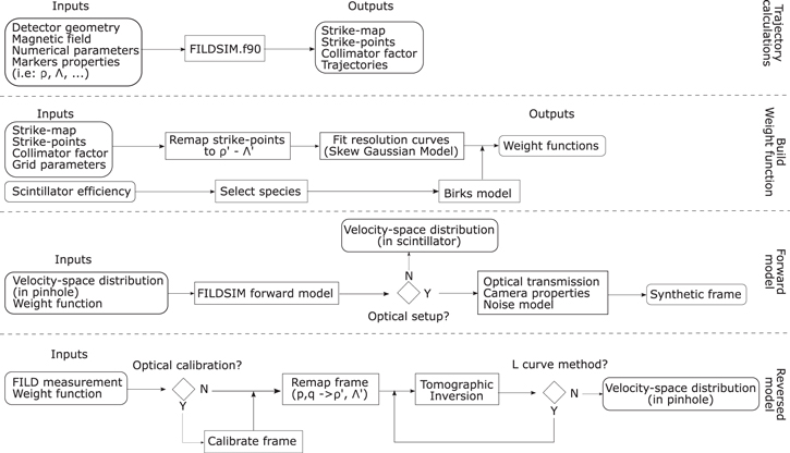
Figure 11. Workflow of the FILDSIM code.
Download figure:
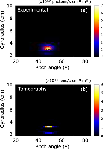
Standard image High-resolution imageWe have selected the signal from FILD1 in AUG shot #32081 at t = 1.14 s for the benchmarking of the model. The FILD experimental signal is shown in figure 12(a), where the velocity-space of the losses measured in the scintillator can be observed. Two different spots at rL ∼ 3.5 cm and rL ∼ 2.5 cm. These are identified as first orbit losses corresponding to the main and half energy component of the NBI source Q7 respectively. The one-third energy component of the NBI ions is blocked by the collimator due to its small gyroradius, and it is therefore not measured. After applying the tomographic inversion to the experimental FILD signal, the undistorted velocity-space of the fast-ion losses at the FILD pinhole is retrieved (figure 12(b)). Two distributions are obtained with a spread in pitch angle ranging from 40° to 60° and very well defined gyroradius of 3.4 and 2.4 cm. The measured pitch angle distribution is given by the pitch angle distribution of the NBI birth profile. These correspond to ions which are born in the edge of the plasma at the low field side. It is worth noticing that these distributions are effectively single energy components and not slowed down energy distributions, as it is expected for the beam ion prompt losses. The deuterium NBI main and half energy components are 93 and 46.5 keV corresponding to gyroradii of 3.2 and 2.3 cm respectively, given the magnetic field at the FILD probe position of 1.93 T. This small discrepancy between the tomographic reconstruction and the expected values of Larmor radii can be due to a misalignment of the strike map. The measured absolute heat flux of these fast-ion losses is ∼1.45 kW m−2.
Figure 12. (a) Photon flux emitted by the scintillator revealing the velocity-space of fast-ion losses measured by FILD1 in AUG #32081 at t = 1.14 s. (b) Retrieved velocity-space of the losses at the FILD pinhole after applying the tomographic inversion to the FILD experimental signal.
Download figure:
Standard image High-resolution image
6. Conclusions
A simple model for the FILD detector response using a weight function formalism based on orbit trajectory calculations has been presented. The measured FILD signal at the scintillator can be interpreted as a distorsion of the velocity-space distribution of the ions reaching the detector pinhole due to the finite resolution of the system. The relation between the measurements and the velocity distribution can be efficiently summarized by so-called weight functions. The weight functions can be expressed as the product of a probability function times the scintillator efficiency, which is measured experimentally. The probability functions are shown to fit well to skewed 2D Gaussian distributions, whose parameters depend only on the geometry of the collimator. Further optimization of the analytical model towards a better fit to the numerical results of the strike-point distributions in the scintillator seems to be possible, although it is left for future work. In particular, the tails of the Gaussian functions in the analytical model presented here could be leading to an underestimation of the detector resolution.
The model allows us to obtain synthetic FILD signals given any velocity-space distribution at the pinhole. This synthetic diagnostic is useful for a direct comparison between simulations and experiments. Furthermore, the formulation of the problem in terms of weight functions allows the efficient inversion of the forward model by the application of velocity-space tomography techniques, such that the undistorted velocity distribution at the pinhole can be recovered. A sensitivity study has been carried out to assess the capabilities and limitations of this technique. It has been shown that the tomography works at realistic Gaussian noise levels typically obtained in FILD signals and is able to differentiate between monoenergetic and energy spread distributions. Finally, the model has been benchmarked against experimental FILD signals of beam ion prompt losses at the ASDEX Upgrade tokamak. It has been shown that the undistorted velocity-space of the fast-ion losses at the FILD pinhole, which is the physically relevant information, can be retrieved by means of the tomographic inversion.The technique can reveal additional details of the velocity-space distribution of the lost ions, which may be of great interest for the study of the velocity-space dynamics of fast-ion losses induced by MHD instabilities. The use of the FILDSIM code has been demonstrated to improve the analysis and interpretation of FILD signals.
The tool presented here constitutes a first step towards the integration of FILD measurements in a common framework including other confined fast-ion diagnostics, with the ultimate goal of achieving the tomographic reconstruction of the full fast-ion distribution function. The combination of different diagnostics in velocity-space tomography is a general problem which has been discussed in previous works [27, 31]. The main challenge is to combine velocity-space measurements which are performed in different volumes of the configuration space. This is of particular importance in the case of FILD, whose probing volume is in the far scrape-off layer, very distant from the plasma volumes probed by confined fast-ion diagnostics, which are inside the separatrix. In this sense, the so-called orbit tomography method [38] could be a good framework to combine the information provided by diagnostics measuring confined and escaping fast-ion populations.
We have presented here single time-slices of tomographic inversions of FILD measurements. However, velocity-space tomography movies based on fast-ion D-alpha measurements [30] have been computed within a few hours, suggesting that FILD data could be analyzed in the same way. Future work will focus on the development of alternative tomographic inversion methods which can potentially improve the time performance.
Acknowledgments
This work was supported by the ITPA Topical Group for Energetic Particle Physics. This research was supported in part by the Spanish Ministry of Economy and Competitiveness through the projects FIS2015-69362-P (MINECO/FEDER,UE), Grant Nos. RYC-2011-09152 and ENE2012-31087 and the Marie Curie FP7 Integration Grant (No. PCIG11-GA-2012-321455). This work has been carried out within the framework of the EUROfusion Consortium and has received funding from the Euratom research and training programme 2014-2018 under grant agreement No 633053. The views and opinions expressed herein do not necessarily reflect those of the European Commission.