

Abstract
Objective. To present the first 3D CGO-based absolute EIT reconstructions from experimental tank data. Approach. CGO-based methods for absolute EIT imaging are compared to traditional TV regularized non-linear least squares reconstruction methods. Additional robustness testing is performed by considering incorrect modeling of domain shape. Main Results. The CGO-based methods are fast, and show strong robustness to incorrect domain modeling comparable to classic difference EIT imaging and fewer boundary artefacts than the TV regularized non-linear least squares reference reconstructions. Significance. This work is the first to demonstrate fully 3D CGO-based absolute EIT reconstruction on experimental data and also compares to TV-regularized absolute reconstruction. The speed (1–5 s) and quality of the reconstructions is encouraging for future work in absolute EIT.
Export citation and abstract BibTeX RIS
1. Introduction
The main objective of this paper is to demonstrate the feasibility, speed, and robustness of producing 3D absolute (static) images of the electrical conductivity inside a tank, from experimental Electrical Impedance Tomography (EIT) data measured on an array of electrodes on the tanks surface by the ACT5 (Rajabi Shishvan et al 2021) adaptive current tomography system, using CGO-based reconstruction algorithms. The primary contributions of this work are that it presents the first use of Complex Geometrical Optics (CGO) based methods to produce absolute (static) images of the conductivity from experimentally measured EIT data in 3D, and studies their robustness under modeling errors.
'Absolute', or 'static', conductivity images are images of the conductivity inside a body made from one set of experimental measurements made on the surface of the body at one time (Denaï et al 2010). Alternatively, 'dynamic', or 'time-difference', imaging uses two sets of data measured at two different times to make an image of the change in the conductivity that took place between the two times the measurements were made. We present both types of images made from experimental data by CGO-based algorithms in 3D in this paper.
Applications of EIT began with geophysical exploration over a century ago (Keller and Frischknecht 1966, Allaud and Martin 1977) and have since expanded into several fields including the transport of fluids and gases (Eggleston et al 1989, Kaipio and Somersalo 2004, Wang 2015), and biomedical imaging (Swanson 1976, Henderson and Webster 1978, Barber and Brown 1984, Holder 2005, Frerichs et al 2017, de Castro Martins et al 2019, Kao et al 2020, Adler and Holder 2021). Systems for monitoring lung function in real-time are now commercially available and clinical trials are in progress to determine the extent to which some of these systems might be used to guide mechanical ventilation (The PLUG group 2022, Brochard 2022, Timpel 2022). These systems typically make and display two dimensional images of the differences in conductivity between two states, e.g., lungs filled with air and lungs depleted of air, in order to take advantage of dynamic (difference) imaging methods and algorithms (Frerichs et al 2017, Adler and Holder 2021). The desire to improve the diagnosis of cancer and stroke has motivated the development of systems and methods capable of imaging the absolute or static internal conductivity and permittivity in 3D (Cherepenin et al 2001, Kerner et al 2002, Choi et al 2007, Kao et al 2007, Goren et al 2018). The interested reader is referred to (Cheney et al 1999) for further review of applications of EIT.
Most absolute (static) EIT reconstruction focuses on solving a simplified linearized problem or iteratively solving an optimization-based method which requires repeated solutions to the forward problem which can become costly for highly dense meshes. CGO-based methods are direct methods in that they do not require iteration. They have the capability to solve the full nonlinear mathematical inverse problem, and do not require repeated solutions to the forward problem, e.g. via the finite element method (FEM). The D-bar inversion algorithm, which is a specific type of CGO-based inversion algorithm in 2D, has been used to make both absolute and difference images in 2D in real-time from experimental data measured on tanks, and for difference imaging on human subjects in laboratory and clinical settings. See Mueller and Siltanen (2020) for a recent review of the 2D D-bar method and its applications, and Nachman (1996) for the theoretical foundation.
In 3D, existence and uniqueness of solutions (Nachman 1988, Novikov 1988) can be shown for a 3D D-bar type equation but the constructive proof, upon which the reconstruction algorithms are built, bypasses the 3D D-bar equation instead using a high (non-physical) frequency limit connecting the nonlinear scattering data and the linear Fourier data. Advances in the numerical implementation of 3D CGO-based methods are more recent. The first numerical implementation of 3D CGO-based methods on simulated electrode data using current injection on the surface of the sphere was presented in Hamilton et al (2021). A 3D CGO-based inversion algorithm, regularization scheme, rigorous proof of stability under certain hypotheses, and examples reconstructing the conductivity inside a sphere from numerically simulated Dirichlet data on the entire surface of the sphere (without electrodes) were given in Knudsen and Rasmussen (2022). Until now it has been an open question if 3D CGO-based algorithms could be used with experimental data. This paper answers this question affirmatively by showing that the conductivity can be recovered rapidly and robustly from experimental data measured on 32 electrodes on the surface of a rectangular prism building on the work of Hamilton et al (2021).
It was demonstrated in Goble (1990), Blue (1997), Holder (2005), Kao et al (2020) that it is possible to make electrical impedance tomography (EIT) Systems that produce both 3D static and dynamic images of the interior of the chest showing heart and lung regions, as well as changes in those regions due to ventilation and perfusion. These systems used linearized and iterative methods. The former are fast but less accurate and the latter are slower. Recent 3D CGO inversion algorithms and their analysis, when applied to synthetic or simulated data, suggested that they have the potential to be fast and more accurate (Delbary and Knudsen 2014, Hamilton et al 2021, Knudsen and Rasmussen 2022). Here we test their capabilities on experimental EIT data.
In this paper we compare the following methods for making static 3D images from experimental tank data, collected by the ACT5 imaging system:
- A CGO linearization method based on Calderóns original proposal introducing CGO ideas into the subject (Calderón 1980). We call this algorithm Calderóns method.
- Two CGO-based methods for solving the full non-linear inversion problem based on Sylvester and Uhlmanns original uniqueness proof and Nachmans constructive uniqueness proof in Sylvester and Uhlmann (1987), Nachman (1988). The first is the
 algorithm, and the second is called t0, (Delbary et al
2012, Hamilton et al
2021) both of which are simplifications of the original constructive proof.
algorithm, and the second is called t0, (Delbary et al
2012, Hamilton et al
2021) both of which are simplifications of the original constructive proof. - A more traditional iterative inversion method based on optimization using a Total Variation (TV) regularization.

The EIT data were measured on 32 electrodes attached to the six surfaces of a rectangular tank using the ACT5 system. The system can adaptively determine patterns of currents to apply to all 32 electrodes that result in voltages on those electrodes that are proportional to the applied currents. These 'eigen currents' form a discrete orthogonal set and provide improved voltage data for reconstructing the conductivity inside the tank from a limited amount of current or power that can be applied to the tank. The theory of adaptive current tomography systems is given in Isaacson (1986), Gisser et al (1990, 1988), Cheney and Isaacson (1992), Li et al (2013, 2014), Newell (2005), Saulnier (2005).
The remainder of the paper is organized as follows. Section 2 provides a brief review of the mathematics of EIT and encompasses the methods used in the work: the CGO and reference reconstruction algorithms, experimental setup for the ACT5 data collection, robustness tests that will be explored, and metrics used to evaluate the results. The results section, section 3, presents slice, 3D, and isosurface renderings of the recovered conductivities for correct and incorrect domain modeling. Section 4 contains a discussion of the results and conclusions are drawn in section 5.
2. Methods
In this work we compare three CGO-based methods (Calderón's Method, the  Method, and the t0 Method) to a more common iterative Total Variation (TV) regularized non-linear least squares method for absolute EIT image reconstruction. For comparison, we also include time difference EIT images for the CGO-based methods and compare them to a linearized difference imaging method. We begin with a brief review of the mathematical problem.
2.1. Mathematical background
The mathematical problem of reconstructing the internal conductivity, when measurements can be made with infinite precision everywhere on the boundary of a body, is currently called 'Calderóns Problem' by much of the mathematical community since A. Calderón formulated this inverse problem as follows (Calderón 1980): In two or more dimensions, can one find the conductivity, σ(x), inside a body, Ω, from all possible electrical measurements made on the surface, ∂Ω, of the body? Here the voltage or potential, u(x), inside the body, due to an applied surface current density, j(x), is assumed to satisfy the following low frequency approximation to Maxwells equations, which we will refer to as the conductivity equation, with a Neumann boundary condition:

Here ν = ν(x) denotes the outward pointing unit normal to the surface at x ∈ ∂Ω, and,  . We denote the mapping from applied current density to resulting voltage on the surface, called the 'Neumann-to-Dirchlet' (ND) map, by
  , where
  for x ∈ ∂Ω, and u(x) solves the conductivity equation (2.1) with Neumann data j(x).
The Calderón problem can also be formulated as the mathematical problem. If one is given the ND map or operator,  , or equivalently its inverse, the Dirichlet-to-Neumann (DN) operator,
  , can one find σ(x)? Calderón showed that if σ(x) does not differ too much from a constant then one can recover an approximation to it from the ND map. His short paper showed this could be done using Fourier Transforms in a very clever way, by introducing special solutions, eζ·x
, to the conductivity equation with constant conductivity, i.e. the Laplace equation, where ζ is a complex valued vector with ζ · ζ = 0. This is possible in two or more dimensions when the conductivity is close to a constant and gave birth to Calderón's method as described in this paper, as well as more powerful methods for solving the full non-linear problem by generalizing Calderóns solutions to what we now call Complex Geometrical Optics (CGO) solutions, introduced by Sylvester and Uhlmann (1986, 1987) in their landmark paper proving that the Calderón problem in three or more dimensions has a unique solution, where the inversion problem is reduced to a Fourier transform in the limit ∣ζ∣ → ∞ . The
, can one find σ(x)? Calderón showed that if σ(x) does not differ too much from a constant then one can recover an approximation to it from the ND map. His short paper showed this could be done using Fourier Transforms in a very clever way, by introducing special solutions, eζ·x
, to the conductivity equation with constant conductivity, i.e. the Laplace equation, where ζ is a complex valued vector with ζ · ζ = 0. This is possible in two or more dimensions when the conductivity is close to a constant and gave birth to Calderón's method as described in this paper, as well as more powerful methods for solving the full non-linear problem by generalizing Calderóns solutions to what we now call Complex Geometrical Optics (CGO) solutions, introduced by Sylvester and Uhlmann (1986, 1987) in their landmark paper proving that the Calderón problem in three or more dimensions has a unique solution, where the inversion problem is reduced to a Fourier transform in the limit ∣ζ∣ → ∞ . The  and t0 methods described below in section 2.3 follow this strategy, as opposed to the 2D D-bar methods described in Mueller and Siltanen (2020). This strategy is not possible in 2D where the CGO solutions are found by solving a first order linear PDE involving D-bar operators in the complex vector ζ and taking it to 0. Constructive proofs using these CGO solutions and D-bar ideas from inverse scattering theory, along with applications to scattering and acoustics were given in Nachman (1988), Novikov (1988).
CGO methods were used to prove uniqueness in the more difficult case of 2D where constructive methods for reconstructing the conductivity were given in detail in Nachman (1996) for  and later in Astala and Päivärinta (2006) for σ ∈ L∞(Ω). Other pioneering work proving uniqueness under a variety of hypotheses on the conductivity include Langer (1933), Tikhonov (1949), Druskin (1982), Kohn and Vogelius (1984), Parker (1984), Novikov (1988). Extensive references to more recent progress in the analysis and numerical analysis of the Calderón problem can be found in Borcea (2002), Mueller and Siltanen (2012), Delbary and Knudsen (2014), Uhlmann (2014), Feldman et al (2019), Mueller and Siltanen (2020), Knudsen and Rasmussen (2022).
In what follows we will be interested in the problem of reconstructing an approximation to the internal conductivity from finitely many experimental measurements made with finite precision. Unfortunately, this is an ill-posed problem and, unlike the purely mathematical problem, it does not have a unique solution. Nevertheless, it is sometimes possible to reconstruct useful approximations to the internal conductivity with a finite number of degrees of freedom, or voxels, which we will illustrate by making images from experimental data and comparing them to the actual interior conductivity within the tanks.
The EIT problem for a body with L electrodes, eℓ
, ℓ = 1, 2,...,L, on its surface, is to find an approximation to the internal conductivity from all the possible electrical measurements made on these L electrodes. In particular we will assume that we apply L − 1 linearly independent patterns of currents,  , k = 1, 2,...,L − 1, to the L electrodes, and measure the resulting L − 1 voltage patterns,
  , where
  and
and  denote the applied current, and measured voltage from the kth pattern, on the ℓth electrode, for ℓ = 1, 2,...,L. From conservation of charge, and our choice of ground, we assume
The kth voltage or potential, u(k)(x), resulting inside the body is determined by the conductivity equation, ∇ · σ∇u(k) = 0, and the 'Complete Electrode Model', (Cheng et al 1989, Somersalo et al 1992) where:
Here zℓ
is the effective contact, or surface, impedance on the ℓth electrode. The current patterns used will be eigenvectors of the Current to Voltage map, which is a matrix approximation to the ND map, for the homogeneous saline tank. They are found numerically by simulating a homogeneous tank for static/absolute imaging, and experimentally by adaptive methods for difference/dynamic imaging. The matrix approximations to the ND maps from the conductivity distribution σ are denoted by the L × L matrices, Rσ
, where  , and we define
  . Here the vectors
  ,
,  , denote vectors all of whose components are 1, or 0, respectively. The discrete analog of the DN map used in the CGO-based methods is given by
  .
.
2.2. Calderón's method
Following Calderón's original paper (Calderón 1980), Calderón's method approximates the conductivity, σ(x), from its Fourier transform. Here we present a brief description of the method and refer the reader to Calderón (1980), Bikowski and Mueller (2008), Muller et al (2017), Hamilton et al (2021) for further details. Calderón's method assumes the conductivity is a small perturbation, δ σ(x), from a constant background, σb , i.e. σ(x) = σb + δ σ(x). In this paper, we assume that the background conductivity σb = 1. If the background constant is not one, then the problem can be scaled and unscaled as in Isaacson et al (2004), Hamilton et al (2021).
The three steps of Calderón's method in 3-D, as described in Hamilton et al (2021), are:
Step 1: Use the DN maps Λσ
and Λ1 to approximate the Fourier transform of the small perturbation in conductivity,  , by
, by

where z and a satisfy

and Λ1 is the DN map for a constant conductivity of 1.
Step 2: Take the inverse Fourier transform of  :
:

Step 3: Add the background to the perturbation to recover the approximate conductivity, σCAL (x):

The definition of the Fourier transform in Calderón's method is different from that used in the  and t0 methods described below. However, each method is consistent with its definition and is consistent with the respective literature on that method.
In this paper, we compute  in spherical Fourier coordinates. As such, we choose

for ∣z∣ ≥ 0,  and
and  so that z and a satisfy (2.4). Then, the inverse Fourier transform in (2.5) becomes

Additionally, we implement the use of a mollifier,  , as introduced in Calderón (1980) for some parameter
  to reduce Gibbs phenomenon caused by jump discontinuities in σ(x) while recovering δ
σCAL
to reduce Gibbs phenomenon caused by jump discontinuities in σ(x) while recovering δ
σCAL

We implement the same mollifier as used in Bikowski and Mueller (2008), Hamilton et al (2021),

where  and t acts as a smoothing parameter with larger t values producing smoother reconstructions with smaller jumps at points of discontinuity in σ(x).
Since noise causes (2.3) to blow up at large ∣z∣, we use a non-uniform truncation regularization strategy. A similar regularization strategy was proved stable for the 2D D-bar method in Knudsen et al (2009), which also noted non-uniform truncation also produces reliable reconstructions. In our case, we will first compute  for ∣z∣ within an outer radius of
  . We keep values of
  whose real and imaginary amplitudes are below a threshold determined by the amplitudes of
  within a smaller radius
 is set to 0 everywhere else. Both radii are chosen empirically. The inner radius
  is chosen as a region in z-space where noise does not cause
  to blow up and
  is chosen to keep as much reasonable information from
  without introducing holes in the non-zero region of
  . As such, our truncated
  is computed by

With our truncated  , equation (2.8) is truncated in the radial variable, leading to the approximation

For difference images shown in this paper, we only perform Steps 1 and 2 of the method and replace Λ1 in (2.3) with a reference DN map,  before computing (2.11). Thus, the flow for absolute images is

and the flow for difference images in this paper is
2.2.1. Numerical implementation
In this section, we review the implementation details of Calderón's method introduced in Hamilton et al (2021).
For Step 1, we compute (2.3) for  by discretizing the boundary integral as follows,
where ∣∂Ω∣ is the surface area of the domain; L is the number of electrodes;  denotes the vector of the Cartesian centers of the L electrodes; T
denotes the traditional, non-conjugate, matrix transpose; Lσ
and L1 denote the discrete matrix approximations to the DN maps Λσ
and Λ1 respectively; and
denotes the vector of the Cartesian centers of the L electrodes; T
denotes the traditional, non-conjugate, matrix transpose; Lσ
and L1 denote the discrete matrix approximations to the DN maps Λσ
and Λ1 respectively; and  denotes an orthonormal basis created using Nli
linearly independent applied currents over L electrodes as was done in Hamilton et al (2021). The matrix L1 is based on the FEM solution of the CEM (2.2). Problem-specific mesh details are given below in section 2.6.
denotes an orthonormal basis created using Nli
linearly independent applied currents over L electrodes as was done in Hamilton et al (2021). The matrix L1 is based on the FEM solution of the CEM (2.2). Problem-specific mesh details are given below in section 2.6.
We then compute  according to equations (2.10) and (2.12). For Step 2, on an equally-spaced 16 × 16 × 16 rectangular grid in x, the conductivity difference
  is computed via (2.11) using a 3D Simpson's rule using
  , and
, and  uniformly-spaced nodes on the
  , and
, and  grids, respectively. As the number of nodes in the Fourier domain increases, so does computation time, but some artefact reduction can be achieved. Empirically, the artefact reduction did not seem significant enough to warrant an increased computational time beyond these parameter choices.
Difference images are computed using (2.11) and (2.12), replacing L1 with a discrete reference DN map,  in (2.12). For the phantom tank experiments in this paper, this reference map is from data collected with a tank filled only with saline matching the experiment and no other inclusions.
The absolute reconstructions of  in this paper are produced using (2.6) replacing σb
with σbest
in this paper are produced using (2.6) replacing σb
with σbest
The solution is then interpolated to a 64 × 64 × 64 rectangular grid.
Following Isaacson et al (2004), σbest is given by

where  is the kth
simulated voltage pattern measured on electrode ℓwith a homogeneous conductivity of 1 S m−1 and
is the kth
simulated voltage pattern measured on electrode ℓwith a homogeneous conductivity of 1 S m−1 and  is the kth
voltage pattern measured on electrode ℓfor the inhomogeneous conductivity σ. The simulated voltages are the same voltages used to compute L1, as described in section 2.6.1.
is the kth
voltage pattern measured on electrode ℓfor the inhomogeneous conductivity σ. The simulated voltages are the same voltages used to compute L1, as described in section 2.6.1.
2.3. The texp and t0 methods
Both the  and t0 methods are derived from the constructive proofs of Nachman (1988), Novikov and Khenkin (1987), Novikov (1988) and involve special solutions called Complex Geometrical Optics (CGO) solutions (Sylvester and Uhlmann 1987). A brief summary is included here for the reader's convenience. For further details see Delbary et al (2012), Hamilton et al (2021), Delbary and Knudsen (2014), Nachman (1988).
Assuming that the conductivity is a constant σc = 1 in a neighborhood of the boundary ∂Ω, the real-valued conductivity equation (2.1) can be transformed to the Schrödinger equation

via the change of variables  and
and  , by extending σ(x) ≡ 1 for all
  . For
. For  , unique CGO solutions exist to the transformed problem

where ψ(x, ζ) ∼ eix·ζ for large ∣x∣ or ∣ζ∣, and

where ζ2 = ζ · ζ and ζ is a purely auxiliary parameter. The conductivity σ(x) can then be recovered from the DN map Λσ as follows.
For each x ∈ ∂Ω and  , solve the Fredholm integral equation of the Second Kind,

where
denotes the Faddeev Green's function (Faddeev 1966). Then, evaluate the scattering data

For ∣ζ∣ large, the Schrödinger potential q(x) can be recovered via the inverse Fourier transform

The conductivity is then recovered by solving the boundary value problem

for  and evaluating
  . This is the full nonlinear reconstruction method.
Replacing the CGO solutions ψ(x, ζ) by their asymptotic behavior eix·ζ in the scattering data (2.17) via

yields a 'Born approximation' typically called the  approximation for EIT. Using this approximate scattering data in place of the fully nonlinear t(ξ, ζ), one proceeds with the recovery of an approximate potential
  via (2.18) and conductivity
  via (2.19). The flow is:

An intermediate approximation can be computed by replacing the Faddeev Green's function Gζ
(x) in the single layer potential, in (2.16), for the traces of the CGOs, with the standard Green's function  for the Laplacian operator. Thus, one solves

for the CGOs ψ0(x, ζ), avoiding the exponentially growing Faddeev Green's function. A corresponding approximation to the scattering data is then computed by using ψ0(x, ζ) in place of ψ(x, ζ) in (2.17) and then continuing to recover q0(x) and σ0(x). The flow is then

We point out that the methods, as outlined above, assumed that the conductivity was a constant σc
= 1 near the boundary of the domain. As mentioned in section 2.2, the problem can be scaled and unscaled as in Isaacson et al (2004), Hamilton et al (2021) when the constant σc
is not one. In practice, we estimate the best-fit constant conductivity fit to the data σbest as given by (2.13). Explicitly, as in (Hamilton et al
2021), we scale the DN map by using  in place of Λσ
, and re-scale at the end using
in place of Λσ
, and re-scale at the end using  and
and  .
.
In this work we consider both the  and t0 methods. We note that this is the first time that t0 has been implemented on non-continuum DN data and the first time that either
  or t0 have been demonstrated on experimental 3D EIT data, for absolute or time-difference EIT imaging.
2.3.1. Numerical implementation
Here we provide the numerical details pertinent to the implementation of the  and t0 algorithms outlined above. As with the Calderón method above, the main idea is to expand functions in the same orthonormal basis Q as described in section 2.2.
Following DeAngelo and Mueller (2010), for each electrode center xℓ , expand ψ(x, ζ) and eix·ζ as

where  denotes the (ℓ, j) entry of Q. Then, the boundary integral equation (2.21) can be approximated as follows
where  denotes the
  extended electrode where
  and the
  are mutually disjoint (Hyvönen 2009). Note the true electrodes need not cover the surface ∂Ω, only the extended (mathematical) electrodes that we will use to discretize the integral. Then, using the expansions from (2.22) in (2.23), we have
where  represents the action of
  on Qj
evaluated at
on Qj
evaluated at  , which can be computed as the
  entry of
  . Define

where we have removed the singularities at xℓ
= yℓ
. Assuming  for each ℓ = 1,...,L, and using (2.25) in (2.24) we find
or in matrix form,
The solution to this equation can be found by solving the following system for the unknowns  ,
,

where  , and I is the identity matrix. If the extended electrodes Eℓ
are not uniform in size, then one could compute as weighted sum replacing the uniform weight
, and I is the identity matrix. If the extended electrodes Eℓ
are not uniform in size, then one could compute as weighted sum replacing the uniform weight  as appropriate.
Next, following Hamilton et al (2021), the scattering data t0(ξ, ζ(ξ)) can be computed for all ∣ξ∣ less than a chosen truncation radius Tξ via

since  , where
  is the same as in section 2.2.1, i.e. a vector storing the centers of the electrodes.
Next, the approximate potential q0 is recovered by computing the inverse Fourier transform of the truncated scattering data t0 using a Simpson's rule in 3D,
Alternatively, one could use an IFFT to achieve additional speedup, taking care with quadrature points and the particular form of the kernel. Following Hamilton et al (2021), the conductivity σ0(x) was recovered by first solving the boundary value problem (2.19), using the PDE toolbox in Matlab using a mesh with approximately 21, 000 3D elements, then computing  . The 3D visualizations were obtained by interpolation to a 64 × 64 × 64 rectangular grid using Matlab's scatteredInterpolant function. The ζ values were computed following the minimal-zeta approach outlined in Delbary and Knudsen (2014). We remark that while the non-existence of exceptional points for the solution of the boundary integral equation (2.16) is proven for large ∣ζ∣ (Sylvester and Uhlmann 1987, Nachman 1988), as well as small ∣ζ∣ (Cornean et al
2006); it is still an open question for the intermediate values required here to perform the computation on a computer.
. The 3D visualizations were obtained by interpolation to a 64 × 64 × 64 rectangular grid using Matlab's scatteredInterpolant function. The ζ values were computed following the minimal-zeta approach outlined in Delbary and Knudsen (2014). We remark that while the non-existence of exceptional points for the solution of the boundary integral equation (2.16) is proven for large ∣ζ∣ (Sylvester and Uhlmann 1987, Nachman 1988), as well as small ∣ζ∣ (Cornean et al
2006); it is still an open question for the intermediate values required here to perform the computation on a computer.
The  reconstructions were obtained in an analogous fashion to those of t0, this time bypassing the boundary integral equation (2.17) and directly computing
where we have replaced the vector of coefficients  with the expansion of the asymptotic behavior of eix·ζ
given by
with the expansion of the asymptotic behavior of eix·ζ
given by ![${{\bf{Q}}}^{{\bf{T}}}\left[{e}^{i{\bf{x}}\cdot \zeta }\right]$](https://content.cld.iop.org/journals/0967-3334/43/12/124001/revision3/pmeaaca26bieqn92.gif) .
.
Difference imaging can be performed with the t0 and  methods by replacing the matrix L1 with
  and computing σdiff(x)=σ(x) − σbest in the final step.
2.4. Reference methods
Total Variation regularized non-linear least squares reconstructions will serve as the reference reconstructions for the CGO-based absolute imaging cases considered here. A classic linear difference imaging scheme, also reviewed below, will serve as the reference for the CGO-based difference images.
2.4.1. Absolute imaging with TV regularization
A widely used numerical approach for absolute EIT is the total variation (TV) regularized non-linear least squares minimization

where U(σ, z) is the finite dimensional forward map,  are the fixed electrode contact impedances obtained from an initialization step of the minimization, Le
is the Cholesky factor of the noise precision matrix of e so that
are the fixed electrode contact impedances obtained from an initialization step of the minimization, Le
is the Cholesky factor of the noise precision matrix of e so that  , scalar valued α is the regularization parameter and TVβ
(σ) is the (smooth) TV regularization functional (Rudin et al
1992)
, scalar valued α is the regularization parameter and TVβ
(σ) is the (smooth) TV regularization functional (Rudin et al
1992)

where β is the (fixed) smoothing parameter. The forward model U(σ, z) in (2.28) is based on the finite element (FEM) discretization of the complete electrode model (Somersalo et al
1992). For details of the FEM model, see Kaipio et al (2000), Vauhkonen et al (1998), Vauhkonen (1997). In the FEM model, the electric conductivity is approximated as a linear combination of the piecewise linear nodal basis functions in a uniform tetrahedral mesh of N nodes, leading to vector of unknowns  , and the electric potential is approximated similarly in a significantly more dense tetrahedral mesh with refinements near the electrodes. The non-linear optimization in (2.28) is solved by a lagged Gauss-Newton method equipped with a line search algorithm. The line search is implemented using bounded minimization such that the non-negativity σ > 0 is enforced. For more details of the method, see Toivanen et al (2021).
The fixed contact impedances z* and initial (constant) conductivity estimate for (2.28) are obtained from the solution of the non-linear least squares problem

where the scalar  is the coefficient of a spatially constant conductivity image σc
1 and
is the coefficient of a spatially constant conductivity image σc
1 and  . The non-linear least squares problem (2.30) is solved by a Gauss Newton optimization.
2.4.2. Linear difference imaging
In linear difference imaging, see e.g. Bagshaw et al (2003), Barber and Seagar (1987), the objective is to reconstruct the change in conductivity between two measurements (V1; V2). The reference linear difference imaging approach of this paper uses linearized approximations of the observation models


where the Jacobian matrix Jσ of U(σ, z*) is evaluated at σ = σ0. With these linearized models, the difference in the measurements becomes

where δ σ = σ2 − σ1 and δ e = e2 − e1. Now, the inverse problem is to reconstruct δ σ based on the difference data δ V and the model (2.33). A widely used formulation for the linear problem is to use the (generalized) Tikhonov regularization with a smoothness promoting regularization functional

where Lδ
e
is the Cholesky factor of the noise precision matrix of δ
e so that  . In this paper, the regularization matrix Lp
is constructed by utilization of a distance based covariance function. More specifically, we set
. In this paper, the regularization matrix Lp
is constructed by utilization of a distance based covariance function. More specifically, we set  , where the (prior covariance) matrix Γp
is constructed using the distance based correlation function (Lieberman et al
2010)
, where the (prior covariance) matrix Γp
is constructed using the distance based correlation function (Lieberman et al
2010)

where the parameter a controls the correlation length and can be solved by setting the distance ∥xi − xj ∥ to a selected value d (e.g. half the radius of the target) and setting Γp (i, j) to the desired covariance for that distance (e.g. 1% of variance).
2.5. Experimental setup
ACT5 (Rajabi Shishvan et al 2021) is a 32 electrode parallel EIT instrument that uses 32 current sources to apply patterns of current to the target and 32 voltmeters to measure the resulting voltages. The current sources in ACT5 adjust the delivered current to compensate for current lost through shunt impedance, including that introduced by the capacitance of cables that connect the instrument to the electrodes, enabling the desired current patterns to be applied with high precision (Saulnier et al 2020). ACT5 can apply sinusoidal currents at frequencies in the range of 11 kHz to 1 MHz with a peak amplitude of 0.25 mA. The voltmeters measure voltages up to 0.5 V peak with a maximum signal-to-noise ratio (SNR) of 96 dB. Because the current source compensates for shunt capacitance of the cables, the system operates with grounded-shield cables (Abdelwahab et al 2020).
A test tank was built from 3/8-inch-thick Plexiglas with interior dimensions of 17.0 cm × 25.5 cm × 17.0 cm. Thirty-two electrodes were fabricated of 16-gauge 316 stainless steel, each 80.0 mm square. The inside surfaces of the tank were milled out in the shape and depth of the electrodes so that the interior surfaces were flat. The nominal gaps between electrodes were 5.0 mm. The 32 electrodes were placed four on each end and six on each side. Bolts through the center of each electrode passed through the Plexiglas, allowing connections to the cables from the ACT5 electronics. Five sides of the tank were glued together, and provision was made to secure the top with threaded rods at all four corners. Access holes of 0.6 mm at various sites in the top to allow threads to suspend targets, and 25-Ga hypodermic needles to complete the filling of the tank after the lid was in place. In use, a mixture of saline at room temperature at the desired background conductivity is made and measured using a Oakton CON 6+ handheld conductivity meter.
Targets were made the day before experiments by adding NaCl and a few drops of food dye to distilled water until the desired conductivity was obtained, as measured by an immersible conductivity meter. The solution was then heated slowly with stirring as 4% agar (Fisher Scientific) was added until the temperature reached 85 °C–90 °C. The mixture was poured into 5.27 cm inside-diameter spherical molds and allowed to harden overnight. Test cells were also filled at this time so the final conductivities could be verified using the ACT5 instrument.
Data were first collected of the tank filled with saline of the desired conductivity (24 mS m−1) with no targets present. Then, targets were added to the tank supported on fine toothpicks from below. Photos were captured of the tank, with each target in place, to verify its/their position (Figure 1). The conductivity values of the spheres used were approximately 290 mS m−1. Averaged data, over 100 frames, were used in the subsequent conductivity reconstructions. The experimental data will be made publicly available on github. 7
Note that even though we are testing on a rectangular prism tank, the mathematical reconstruction algorithms are not limited to this geometry.
2.6. Robustness tests
In addition to testing the reconstruction methods with the correct domain modeling, we consider a moderate, as well as strong, mis-modeling of the domain. The incorrect domain modeling comes into play in the following places for the CGO-based methods. First in the simulation of the L1 DN data that requires solving the forward EIT problem with a known conductivity σ ≡ 1 S m−1 and the applied current patterns. Next, the incorrect domain modeling presents as incorrect information about the centers of the electrodes x and surface area for the domain ∣∂Ω∣; the subsequent reconstructions of σCAL
,  , and σ0 are recovered on the incorrect domain. For the TV regularized method, the incorrect domain modeling is present in the FEM based forward map U(σ, z) used in the minimization problem (2.28) and computational mesh. For the linear difference imaging method, the incorrect domain modeling is present in the Jacobian matrix of the forward map Jδ
σ
in the minimization problem (2.34) and computational mesh.
, and σ0 are recovered on the incorrect domain. For the TV regularized method, the incorrect domain modeling is present in the FEM based forward map U(σ, z) used in the minimization problem (2.28) and computational mesh. For the linear difference imaging method, the incorrect domain modeling is present in the Jacobian matrix of the forward map Jδ
σ
in the minimization problem (2.34) and computational mesh.
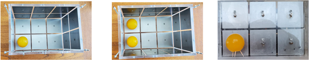
Figure 1. Experimental setups. Left: Top view of the one target experiment. Middle: Top view of two target experiment. Right: side view of height of targets above floor of tank. Note that the targets were measured at 290 mS m−1 in test cells.
Download figure:
Standard image High-resolution imageAccurate domain modeling can be challenging in practice. To address this we explored a domain with a moderately incorrect domain shape, 18cm x 27cm x 19 cm, as well as a domain with a significantly incorrect domain shape, 20 cm × 35 cm × 25 cm 8 . Electrodes were uniformly distributed as in the original box design, but clearly had different locations and spacing than the truth due to the new box dimensions. Figure 2 (center and right) depict the larger box domains. Each reconstruction method was then tested assuming that the actual experimental voltage and current measurements were coming from the boxes shown in figure 2.

Figure 2. 3D renderings of simulated boxes used in robustness testing.
Download figure:
Standard image High-resolution imageTime-difference reconstructions were performed using basal measurements with only 24 mS m−1 saline in the experimental tank. This data was then used in the reconstruction methods discussed in section 2.3.1 and section 2.4.2.
2.6.1. Forward modeling and regularization parameters
For the CGO-based methods, the matrix approximation L1 to the DN map Λ1 was formed using simulated voltage data, using EIDORS (Vauhkonen 1997, Adler and Lionheart 2006). The EIDORS data is produced by solving the forward conductivity problem with the finite element approximation of the Complete Electrode Model (2.2) with σ ≡ 1 Sm−1. In each domain modeling case, see figure 2, the forward problem was solved on a box of the corresponding dimensions, with 8 cm by 8 cm electrodes, using approximately 250,000 nodes and 1.2 million elements with high refinement used near the electrodes, and the default contact impedance in EIDORS. For the reference methods, the FEM based forward problem was solved using the same meshes for the electric potential as with the CGO-based methods and the conductivities were approximated in sparser, uniform meshes with 8,918; 9,410; 14,678 nodes and 43,690; 45,106; 72,438 elements, respectively, for the different domain modeling cases.
The regularization parameters for each of the reconstruction methods were chosen as follows. The regularization parameters  and
and  for Calderón's method were empirically chosen to be 1.4 and 1.7, respectively, and the mollifying parameter was chosen to be t = 0.1 for all reconstructions. These values were chosen empirically to provide the best visual reconstructions. The truncation radius Tξ
for the nonlinear scattering data used in the
for Calderón's method were empirically chosen to be 1.4 and 1.7, respectively, and the mollifying parameter was chosen to be t = 0.1 for all reconstructions. These values were chosen empirically to provide the best visual reconstructions. The truncation radius Tξ
for the nonlinear scattering data used in the  and t0 methods was chosen empirically in the range [10.5, 12] for each case shown here. The localization of the target(s) did not appear to change significantly with Tξ
, however the contrast does appear sensitive to this parameter choice. Further discussion is given below in section 4. For the total variation regularized method, the regularization parameter α and the smoothing parameter β were selected by computing a series of reconstructions with varying α and β values, in the range [1e-6, 100] for α and [1e-4, 0.1] for β, and by choosing the parameters that gave the best visual quality of reconstructions in the correct domain model case. The chosen values α = 0.01 and β = 0.001 were used in all the test cases with different domain models. For the linear difference imaging method, the visually best reconstructions were obtained using a standard deviation of conductivity std(σ) = 16σ0 and parameter a calculated using a covariance of 1% of the variance at a correlation distance d = lbox/8, where lbox is the length of the longest side of the box that is used as the domain model.
and t0 methods was chosen empirically in the range [10.5, 12] for each case shown here. The localization of the target(s) did not appear to change significantly with Tξ
, however the contrast does appear sensitive to this parameter choice. Further discussion is given below in section 4. For the total variation regularized method, the regularization parameter α and the smoothing parameter β were selected by computing a series of reconstructions with varying α and β values, in the range [1e-6, 100] for α and [1e-4, 0.1] for β, and by choosing the parameters that gave the best visual quality of reconstructions in the correct domain model case. The chosen values α = 0.01 and β = 0.001 were used in all the test cases with different domain models. For the linear difference imaging method, the visually best reconstructions were obtained using a standard deviation of conductivity std(σ) = 16σ0 and parameter a calculated using a covariance of 1% of the variance at a correlation distance d = lbox/8, where lbox is the length of the longest side of the box that is used as the domain model.
2.7. Evaluation metrics
As the main focus of this work is experimental data reconstruction, comparing to a known 'truth' with zero error is not possible. The conductivity values for the targets were measured at approximately 290 mS m−1 and the targets were placed to be roughly centered in a sub-cube of the overall box. These data allow us to approximate the localization error (LE) of our reconstructions and maximum conductivity in each reconstructed target.
LE, as in Hamilton et al (2021), measures the distance between the centroids of the reconstructed targets and those of the true targets by

A localization error of 0 is ideal, and signifies the targets are reconstructed in the correct location. In our experiments, the centers of the spherical targets were placed at the centers of the nearest electrode in each direction and in (2.36),  is our best estimate of the true location of the target center, acknowledging possible errors within millimeters of the truth. Following Hamilton et al (2021), to obtain the centers of the reconstructed targets, we use a thresholded segmentation of the reconstructions to identify targets with MATLAB's regionprops3. The thresholds for segmentation were used to empirically identify regions with more than a certain percentage of the maximum reconstructed conductivity. We note that the volume of the segmented targets changes with the choice of threshold, but as we increase the percentage (i.e. threshold) the locations of the centroids stabilize (up to millimeters), from which we computed the LE.
As a major focus of this work is to study how the algorithms tolerate modeling errors, we report a scaled version of the LE,

where we have divided the LE from (2.36) by 25.5 cm, the length of the longest side of the true tank. This scaling value for the computing the LE metric is kept fixed across incorrect modeling scenarios.
3. Results
We first present absolute EIT reconstructions with correct domain modeling, for the one and two targets, and for the four reconstruction methods (figure 3). Cross-sections in the center of the bottom row of electrodes of the box are shown on the left; this slice cuts through the center(s) of the physical target(s). Isosurfaces, shown in the middle column, are extracted from the 3D reconstructions to indicate the locations, size, and number of targets. The isosurfaces were extracted using MATLAB's regionprops3 with threshold segmentation in the range of 60% to 85% of the maximum recovered conductivity in the tank. A uniform threshold across all examples and reconstruction methods was not used as the blurring varied across methods. Note that since the isosurfaces are dependent on this threshold, they can omit information from the full reconstruction. Therefore, the third column shows a full 3D rendering of conductivity in the domain. This 3D rendering is produced in MATLAB by displaying 100 equally-spaced x1-x3 slices set to 0.1 transparency of each slice.
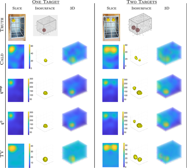
Figure 3. Absolute image reconstructions comparing the CGO methods to the regularized method with correct domain modeling. Slices, isosurfaces, and 3D renderings of the conductivity are shown. Note the truth targets had a measured conductivity of approx 290 mS m−1.
Download figure:
Standard image High-resolution imageFigure 4 shows the absolute EIT reconstructions for the moderately mismodelled domain whereas figure 5 shows the absolute EIT reconstructions for the significantly mismodelled domain. Difference images are shown in figure 6. Metrics of maximum conductivity per target and scaled localization error are shown in tables 1 and 2 for the absolute images and table 3 for the difference images. Bolded entries correspond to the best metric value in each row.
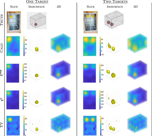
Figure 4. Absolute image reconstructions comparing the CGO methods to the regularized method with moderately incorrect domain modeling, using a box of size 18 cm × 27 cm × 19 cm. Note the truth targets had a measured conductivity of approx 290 mS m−1.
Download figure:
Standard image High-resolution image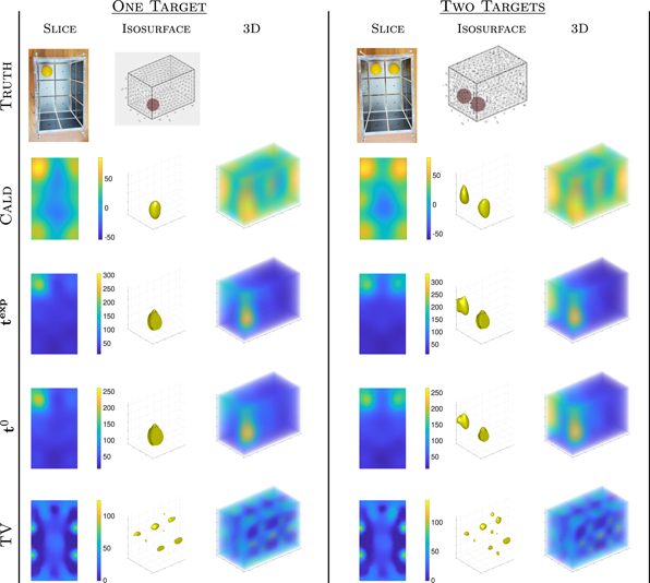
Figure 5. Absolute image reconstructions comparing the CGO methods to the regularized method with largely incorrect domain modeling, using a box of size 20 cm × 35 cm × 25 cm. Note the truth targets had a measured conductivity of approx 290 mS m−1.
Download figure:
Standard image High-resolution image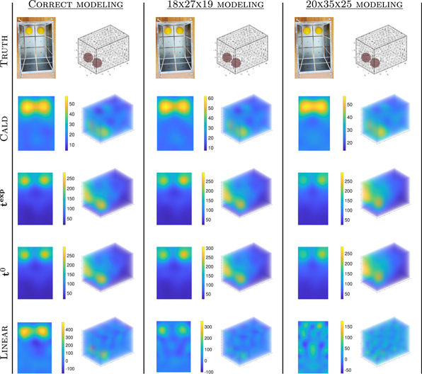
Figure 6. Difference image reconstructions comparing the CGO methods to a typical linear method. Slices and 3D renderings of the conductivity are shown for the correct domain modeling, and increasing levels of error in domain modeling. Note the truth targets had a measured conductivity difference from the background of approx 266 mS m−1.
Download figure:
Standard image High-resolution imageTable 1. One target absolute imaging evaluation metrics across all domain modeling scenarios.
| Calderón |

| t0 | TV | ||
|---|---|---|---|---|---|
| Scaled LE | correct domain | 0.042 | 0.094 | 0.098 | 0.043 |
| box 18 × 27 × 19 | 0.075 | 0.131 | 0.119 | 0.021 | |
| box 20 × 35 × 25 | 0.241 | 0.250 | 0.231 | n/a | |
| Max. Target Conductivity (mS/m) | correct domain | 63.77 | 300.00 | 308.67 | 44.26 |
| box 18 × 27 × 19 | 76.94 | 303.32 | 284.67 | 70.14 | |
| box 20 × 35 × 25 | 85.51 | 305.63 | 260.88 | n/a |
Table 2. Two target absolute imaging evaluation metrics across all domain modeling scenarios. Note: Target 1 is the same target as in the one-target case.
| Calderón |

| t0 | TV | |||
|---|---|---|---|---|---|---|
| Scaled LE | Target 1 | correct domain | 0.056 | 0.098 | 0.105 | 0.034 |
| box 18 × 27 × 19 | 0.103 | 0.135 | 0.133 | 0.021 | ||
| box 20 × 35 × 25 | 0.268 | 0.267 | 0.257 | n/a | ||
| Target 2 | correct domain | 0.062 | 0.195 | 0.180 | 0.031 | |
| box 18 × 27 × 19 | 0.120 | 0.191 | 0.214 | 0.057 | ||
| box 20 × 35 × 25 | 0.277 | 0.311 | 0.295 | n/a | ||
| Max. Target Conductivity (mS/m) | Target 1 | correct domain | 55.61 | 310.95 | 315.50 | 55.57 |
| box 18 × 27 × 19 | 73.53 | 216.29 | 322.39 | 68.29 | ||
| box 20 × 35 × 25 | 80.00 | 334.58 | 264.72 | n/a | ||
| Target 2 | correct domain | 60.47 | 234.85 | 226.35 | 53.94 | |
| box 18 × 27 × 19 | 67.94 | 153.82 | 203.84 | 64.22 | ||
| box 20 × 35 × 25 | 77.81 | 285.06 | 244.80 | n/a |
Table 3. Two target difference imaging evaluation metrics across all domain modeling scenarios. Note: Target 1 is the same target as in the one-target case.
| Calderón |

| t0 | Linear | |||
|---|---|---|---|---|---|---|
| Scaled LE | Target 1 | correct domain | 0.034 | 0.095 | 0.103 | 0.049 |
| box 18 × 27 × 19 | 0.022 | 0.116 | 0.124 | 0.065 | ||
| box 20 × 35 × 25 | 0.113 | 0.242 | 0.243 | n/a | ||
| Target 2 | correct domain | 0.053 | 0.100 | 0.094 | 0.050 | |
| box 18 × 27 × 19 | 0.043 | 0.116 | 0.115 | 0.029 | ||
| box 20 × 35 × 25 | 0.112 | 0.230 | 0.233 | n/a | ||
| Max. Target Conductivity (mS/m) | Target 1 | correct domain | 57.18 | 277.83 | 295.63 | 484.83 |
| box 18 × 27 × 19 | 61.72 | 272.80 | 282.05 | 227.95 | ||
| box 20 × 35 × 25 | 56.30 | 253.46 | 243.88 | 227.95 | ||
| Target 2 | correct domain | 53.84 | 266.91 | 284.25 | 490.88 | |
| box 18 × 27 × 19 | 59.91 | 294.17 | 306.30 | 208.05 | ||
| box 20 × 35 × 25 | 55.07 | 293.61 | 282.38 | n/a |
4. Discussion
Beginning with the correct domain modeling scenario, each method, Calderón,  , t0, and TV produced reconstructions that clearly show the target(s) with good localization. The TV images are sharpest, as expected. The
  and t0 methods achieved the best contrast and best approximated the estimated experimental conductivity. The Calderón and TV methods achieved lower contrast but better scaled localization error. Notably, as shown in figure 6, in terms of artefacts, the absolute CGO reconstructions are as clean as their corresponding difference images. The CGO methods required simulated voltages data for the same experimental setup but with a conductivity σ ≡ 1 S m−1. Even though this data was not tuned to the EIT machine (noise and contact impedances) the methods produced high quality absolute reconstructions.
Moving into incorrect domain modeling, we see all methods handled the moderate domain mismodeling quite well and the CGO methods handled the severe domain mismodeling as well. No significant boundary artefacts are seen in the CGO reconstructions for the 18 cm × 27 cm × 19 cm and only moderate boundary artefacts in the TV reconstructions. In the more severe mis-modeling case, assuming the data is coming from a much larger box (20 cm × 35 cm × 25 cm) instead of the true domain (17 cm × 25.5 cm × 17cm), the  and t0 methods still produce good reconstructions showing the correct number of targets and correct region of the tank. The localization is worst in the x3 direction showing the targets slightly elongated. While artefacts in the Calderón 20 × 35 × 25 reconstructions are present, the method still does detect the true objects as the most conductive. The TV algorithm failed to identify any of the targets for both cases with the 20 × 35 × 25 box. The artefacts in the TV reconstructions in these cases with incorrect domain model could be expected as the regularized non-linear least squares minimization-based absolute imaging EIT algorithms are known to be highly sensitive to modeling errors such as errors in modelling of the domain shape, see e.g. Nissinen et al (2010), Kolehmainen et al (2008), Lehikoinen et al (2007).
We can see the effect of the underlying assumption for Calderón's method that the conductivity is a small perturbation from a constant. In the physical experiments, the conductor(s) had roughly twelve times the conductivity of the background saline. This is seen in the underestimation of maximum conductivity from Calderón's method. However, unsurprisingly, this method does a good job of localizing the targets, in all cases except for the absolute image from the significant domain modeling error. The artefacts seen in the Calderón reconstructions are consistent with what has been observed for absolute imaging with Calderón in 2D, such as Gibbs phenomenon for all absolute reconstructions and higher reconstructed conductivity at electrode locations when the domains were incorrectly modelled. Across all modeling scenarios, the regularized TV method struggled with the high contrast targets, giving maximum target conductivities well below the measured values. The same effect was seen in simulated scenarios where, however, maximum conductivities of lower contrast targets were reliably recovered. This is at least partially explained by saturation of contrast distinquishability of the measurements, i.e. the effect of increasing the conductivity of the target inclusion on the measurements gradually diminishes and until certain level the TV regularized method can no longer discern between high and even higher conductivities.
We note that the electrodes used in this experiment were very large and the structure of the domain, a box with corners, may exacerbate some of the modeling and/or hardware challenges. Nevertheless, the study provides informative results on the feasibility of absolute EIT reconstruction in 3D.
The difference images from Calderón are able to handle the stronger mismodeling of the domain, as are the  and t0 methods. The strong mismodeling proved too severe for the linear difference imaging reference method, which did not manage to identify the targets, see figure 6.
While the  and t0 CGO methods did reliably recover the contrast and approximate location of the targets across examples studied here, they do appear more sensitive than their 2D D-bar based counterparts in regards to the regularization parameter, Tξ
, used in the truncation of the nonlinear scattering data. Figure 7 displays the effect that Tξ
plays on the scaled localization error and maximum recovered conductivity value for the single target, correct domain modeling case. Recall that a secondary nonuniform truncation is also enforced where scattering data with magnitudes exceeding 20 for the real or imaginary parts are set to zero. Adjusting that value will also have an effect on the reconstruction. The value of 20 was chosen in this work for its overall reliability across examples. The contrast appears more sensitive than the localization error. As in Delbary and Knudsen (2014), the minimum ζ parameterization of ξ was used, as the scattering data is a function of both
and t0 CGO methods did reliably recover the contrast and approximate location of the targets across examples studied here, they do appear more sensitive than their 2D D-bar based counterparts in regards to the regularization parameter, Tξ
, used in the truncation of the nonlinear scattering data. Figure 7 displays the effect that Tξ
plays on the scaled localization error and maximum recovered conductivity value for the single target, correct domain modeling case. Recall that a secondary nonuniform truncation is also enforced where scattering data with magnitudes exceeding 20 for the real or imaginary parts are set to zero. Adjusting that value will also have an effect on the reconstruction. The value of 20 was chosen in this work for its overall reliability across examples. The contrast appears more sensitive than the localization error. As in Delbary and Knudsen (2014), the minimum ζ parameterization of ξ was used, as the scattering data is a function of both  and
and  in 3D instead of just
  as in 2D D-bar based methods. Alternative parameterizations and a more detailed study of the effect of the regularization parameters, while interesting, are outside the scope of this work.

Figure 7. Comparison of the effect of the truncation value Tξ
of the scattering radius in the  and t0 CGO methods for Scaled Localization Error (left) and Maximum value of the recovered target. Max conductivity values (right) for Tξ
= 11, 11.5, off the plot, spiked into the 1500–5000 mS m−1 range.
and t0 CGO methods for Scaled Localization Error (left) and Maximum value of the recovered target. Max conductivity values (right) for Tξ
= 11, 11.5, off the plot, spiked into the 1500–5000 mS m−1 range.
Download figure:
Standard image High-resolution image
In terms of speed, when running reconstructions on a MacBook Pro with a 2.3 GHz Dual-Core Intel ® Core i5 processor, Calderón reconstructions on a 16 × 16 × 16 x-grid which are interpolated to a 64 × 64 × 64 x-grid take 1 to 2 seconds without optimizing for parallelization. This increases to 6–8 seconds per reconstruction when the initial x-grid is 32 × 32 × 32. When running on a PC with a AMD EPYC 7702P 64-Core Processor 2.00 GHz, the reconstruction times are 0.6–0.7 seconds and 4 seconds, respectively, again without optimizing for parallelization. On an 2015 iMac with a 4 GHz Quad-Core Intel ® Core i7 processor, the  and t0 methods require 3–4 seconds/recon using a 21 × 21 × 21 x-grid for the potential q(x) or 6–8 seconds/recon when using a 41 × 41 × 41 x-grid for q(x). The timings are non-optimized with the highest computational cost coming from computing the inverse Fourier transform and solving the boundary value problem using FEM. The regularized TV, and linear difference, reconstructions averaged 2–3 hrs, and 3 minutes, respectively, when computed on a server with 256 GB of RAM and two 10 core Intel ® Xeon ® CPU E5-2630 v4 @2.20 GHz processors. We remark that the rather long computation times of the TV regularized non-linear least squares approach are caused by the 3D problem with a computationally rather challenging geometry as the sufficient accuracy of the CEM forward model (2.2) necessitates significant mesh refinement near the electrodes, leading to the large number of degrees of freedom (approx 250,000 nodes) in the FEM based forward model. The FEM model needs to be solved multiple times in the line search at each iteration of the Gauss-Newton method and with the mesh used each forward solution takes approximately 80s computation time.
5. Conclusions
In this work, we presented the first 3D absolute EIT reconstructions from CGO-based methods on experimental 3D tank data, and compared them to the current standard, a total variation regularized non-linear least squares approach. We demonstrated that, with correct domain modeling, quality 3D absolute reconstructions can be obtained by all of the methods, comparable to the quality seen in linear difference imaging. All methods, Calderón,  , t0, and TV reasonably handled the moderate domain modeling error within little noticeable change in localization error and target contrast. For the large modeling error case, the
  and t0 methods correctly identified the targets with high contrast, additional artefacts were introduced into the Calderón reconstruction, and the error proved too significant for the TV method. The computational cost of the CGO reconstruction is trivial compared to TV (non-optimized, less than 1 sec/recon for Calderón, approximately 5 sec/recon for
  and t0, compared to 2–3 hours per reconstruction for TV).
Acknowledgments
Research reported in this paper was supported by the National Institute of Biomedical Imaging and Bioengineering of the National Institutes of Health under award numbers R21EB028064 (SH and JN) 1R01EB026710-01A1 (GS, DI, JN, ORS, and the development of the ACT5 device). The content is solely the responsibility of the authors and does not necessarily represent the official views of the National Institutes of Health. JT and VK were supported by the Academy of Finland (Project 336791, Finnish Centre of Excellence in Inverse modeling and Imaging), the Jane and Aatos Erkko Foundation and Neurocenter Finland.
Footnotes
- 7
- 8
Due to the smaller ratio of longest side to shortest side, the 16 × 16 × 16 X-grid used for Calderón's method as mentioned in section 2.2.1 does not capture the whole domain, so a 32 × 32 × 32 x-grid is used in the significantly incorrect domain case.