

Abstract
Objective. Investigation of the night-to-night (NtN) variability of pulse oximetry features in children with suspicion of Sleep Apnea. Approach. Following ethics approval and informed consent, 75 children referred to British Columbia Children's Hospital for overnight PSG were recorded on three consecutive nights, including one at the hospital simultaneously with polysomnography and 2 nights at home. During all three nights, a smartphone-based pulse oximeter sensor was used to record overnight pulse oximetry (SpO2 and photoplethysmogram). Features characterizing SpO2 dynamics and heart rate were derived. The NtN variability of these features over the three different nights was investigated using linear mixed models. Main results. Overall most pulse oximetry features (e.g. the oxygen desaturation index) showed no NtN variability. One of the exceptions is for the signal quality, which was significantly lower during at home measurements compared to measurements in the hospital. Significance. At home pulse oximetry screening shows an increasing predictive value to investigate obstructive sleep apnea (OSA) severity. Hospital recordings affect subjects normal sleep and OSA severity and recordings may vary between nights at home. Before establishing the role of home monitoring as a diagnostic test for OSA, we must first determine their NtN variability. Most pulse oximetry features showed no significant NtN variability and could therefore be used in future at-home testing to create a reliable and consistent OSA screening tool. A single night recording at home should be able to characterize pulse oximetry features in children.
Export citation and abstract BibTeX RIS

Original content from this work may be used under the terms of the Creative Commons Attribution 4.0 licence. Any further distribution of this work must maintain attribution to the author(s) and the title of the work, journal citation and DOI.
Abbreviations
| AHI | Apnea-hypopnea index |
| FNE | 'First night effect' |
| HF | High frequency (0.15–0.4 Hz) |
| HRV | Heart rate variability |
| LF | low frequency (0.04–0.15 Hz) |
| LMM | linear mixed models |
| MOS | McGill oximetry score |
| nHF | normalized HF |
| nLF | normalized LF |
| NtN | Night-to-night |
| ODI | Oxygen desaturation index |
| ODI1 | Oxygen desaturation index lasting for 1 s |
| ODI5 | Oxygen desaturation index lasting for 5 s |
| ODI10 | Oxygen desaturation index lasting for 10 s |
| OSA | Obstructive sleep apnea |
| Pm | Power in the modulation band |
| PO | Phone oximeter |
| PPG | photoplethysmography |
| PPI | Pulse to pulse interval |
| Pratio | Ratio between Pm/Ptot |
| PRV | Pulse rate variability |
| PSG | polysomnography |
| Ptot | Total power |
| RMSSD | Root mean square of the successive differences between adjacent PPIs |
| SDB | Sleep disordered breathing |
| SMS | Screen-my-sleep |
| SpO2 | Blood oxygen saturation |
| SQI | Signal quality index |
| SQP | Signal quality percentage |
| std | Standard deviation |
| t90% | Cumulative time spent below 90% |
| t94% | Cumulative time spent below 94% |
| t96% | Cumulative time spent below 96% |
| VLF | Very low frequency (0.01–0.04 Hz) |
1. Introduction
Obstructive sleep apnea (OSA), a common health problem, is characterized by repeated upper airway obstructions resulting in cessations of breathing. These complete (apnea) or partial (hypopnea) cessations of breathing disrupt normal ventilation during sleep. OSA currently affects up to 3% of children (Ali et al 1993, Redline et al 1999, Anuntaseree et al 2001, Rosen et al 2003, Wildhaber and Moeller 2007), up to 22% of adolescents (Johnson and Roth 2006) and from 9% to 38% of the general adult population (Punjabi 2008, Franklin and Lindberg 2015, Senaratna et al 2017). These cessations can result in arousals, frequent sleep fragmentations and oxyhemoglobin desaturations, leading to daytime sleepiness. In children this can lead to behavioral problems, growth failure and developmental delays and therefore, OSA is a serious threat to healthy development of children and their overall well-being. When left untreated, OSA can also result in other serious consequences including cognitive impairment, failure to thrive and cardio-respiratory problems (Pediatrics 2002, Huang et al 2014).
The current gold standard to diagnose and determine OSA severity in children is polysomnography PSG (Chervin 1999, Deutsch et al 2006). PSG requires an overnight stay in the hospital to measure electroencephalography (EEG), electrocardiography (ECG), electromyography, chest movements, pulse oximetry, nasal airflow and video/audio recordings. Because of increasing prevalence of OSA (Franklin and Lindberg 2015) and the current resource intensive overnight diagnosis, PSG is associated with long waiting lists, resulting in a likely underdiagnosis of OSA.
At home screening could provide a non-invasive and simple alternative to investigate the OSA severity in the comfort of the patients' home. Pulse oximetry, part of standard PSG, is a simple and non-invasive method of measuring blood oxygen saturation (SpO2) using a finger probe. Overnight oximetry recordings have previously been explored as an OSA screening tool. An example tool is the McGill oximetry score (MOS), a validated severity scoring system which use overnight oximetry as a tool to prioritize the adenotonsillectomy surgical list (Nixon et al 2004).
The phone oximeter (PO) is another example of an OSA screening tool that provides a platform for overnight oximetry recordings (Karlen et al 2011, Petersen et al 2013). The PO consists of a pulse oximeter combined with a mobile phone, providing both spO2 and photoplethysmography (PPG) signals (a signal that provides an indication of blood volume changes in tissues).
The recorded spO2 signal measures the fluctuations and desaturations in blood oxygen saturation due to apneas. Children with significant sleep disordered breathing (SDB) were successfully screened using overnight features extracted from the spO2 signal (Álvarez et al 2013, Garde et al 2013).
However, there are some apnea events that occur without these desaturations, and therefore, additional methods have been investigated to improve the detection of OSA. OSA has been reported to affect the normal variation of heart rate (Montesano et al 2010, Chouchou et al 2014) and the heart rate variability (HRV), which can help identify OSA events (Peiteado-Brea et al 2014).
Pulse rate variability (PRV) is an estimation (with a confirmed correlation) of HRV that is measured from a PPG signal (Gil et al 2010). A successive study using the PO, showed that combining information from both overnight spO2 and PRV analysis can improve the assessment of OSA in children (Dehkordi et al 2013, Garde et al 2014).
However, all these studies were either performed at the hospital simultaneously to PSG while under the supervision of a sleep technician or performed at home. To our knowledge, no studies compared the variability of pulse oximetry features recorded with the same tool at different locations (hospital and home) in children. The real setting for the proposed PO based OSA screening tool is at home, without clinical supervision. However currently these screening tools are compared with the outcome of hospital PSG. The current study was performed to investigate possible differences in sleep and OSA features due to methodology (at home versus hospital). Specifically, this study was conducted to test our hypothesis, that hospital recordings affect subjects normal sleep and OSA severity and therefore is a risk of sleep apnea underestimation by using at home monitoring tools.
Therefore, in order to explore the utility of PO at home, this study focuses on the variability of sleep apnea features, because this could affect the outcome of models based on these features. Were we expect that this variability can occur due to several causes such as physiological, pathological or other conditions (e.g. temperature, emotion, daily activity). The aim of this study is to compare the variability of sleep apnea parameters of the oximetry signal (e.g. oxygen desaturation index (ODI), spO2 saturation, maximal spO2 drop, number of oxygen desaturations), and HRV features in children when collected in hospital and over multiple nights at home.
2. Materials
2.1. Dataset
The screen-my-sleep (SMS) dataset was created to clinically validate the PO as an at-home OSA screening and assessment tool for children (Hoppenbrouwer et al 2018). The data was collected at the British Columbia Children's Hospital (BCCH), Vancouver, Canada, during an overnight stay in a specialized sleep lab. Following ethics approval of study protocol (H14-02241), 75 children suspected with OSA and referred for overnight PSG measurement were recruited between June 2015 and March 2016 (Hoppenbrouwer et al 2018). One patient withdrew from the study. After the overnight stay in the hospital with simultaneous recordings with both PSG and PO, the patients were asked to record at least two additional nights at home with only the PO. With these multiple recordings, the night-to-night (NtN) variability of oximetry features was investigated.
Table 1 summarizes the demographic information (mean and standard deviation (std)) of the entire SMS dataset at an apnea-hypopnea index (AHI) cut-off of 5. There were no significant differences between both groups in demographics, age and BMI, evaluated by a t-test at p < 0.05.
Table 1. Demographic information of the complete SMS dataset (mean (standard deviation (std))). No significant differences were found between both groups.
| Total | OSA | nonOSA | |
|---|---|---|---|
| Children (n) | 74 | 28 | 46 |
| Male (Female) | 38 (36) | 11 (17) | 27 (19) |
| Age | 8.3 (3.9) | 7.2 (4.2) | 9.0 (3.7) |
| BMI | 20.0 (6.3) | 19.0 (4.5) | 20.6 (7.2) |
2.2. Study protocol
The PSG recordings were recorded by an Embla Sandman S4500, with the following signals: ECG, EEG, chest movements, pulse oximetry, nasal and oral airflow and audio/video recordings. The PO was placed on the opposite finger or toe and recordings consisted of spO2 (0.1% resolution) and PPG signals with respectively a sampling frequency of 1 Hz and 62.5 Hz.
3. Methods
3.1. Signal analysis
Signal analysis consisted of extracting oximetry features from the overnight spO2 and PPG signals, both in time and spectral domain. Both analyses consisted of investigating (1) overall features extracted over the total night to provide overnight information; and (2) of additional window-by-window characterization of the signals using time and frequency features (see figure 1). The window-by-window features were extracted by partitioning the whole registration in non-overlapping windows of 2 min. Time and spectral features were extracted from each window. The statistical distribution of all windows over the whole night were then evaluated through the mean, median, standard deviation and interquartile range to provide the final features. All overnight recordings were analyzed using MATLAB R2019b (Mathworks Inc, Natick, USA).
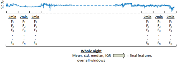
Figure 1. Overview of the window-by-window analysis and the feature extraction. The window-by-window features were extracted by partitioning the whole registration in non-overlapping windows of 2 min. Time and spectral features (F1, F2, ... FN , where N the number of features) were extracted from each window. The statistical distribution of all windows over the whole night were then evaluated through the mean, median, standard deviation and interquartile range to provide the final features.
Download figure:
Standard image High-resolution image3.1.1. Data preparation
Preparation of the dataset consisted of firstly combining measurements recorded during the same night and secondly, because both spO2 and especially PPG analysis are sensitive to artifacts, a signal quality index (SQI) for both signals was calculated to exclude the windows of the signal containing artifacts. Only measurements with a minimum duration of good quality signal of 3 h per night were considered.
3.1.2. SpO2 characterization
Before further analysis, the SQI was determined. All spO2 samples below 70% or above 100% were considered artifacts, and spO2 windows where more than 50% of the samples were artifacts were removed from further analysis.
3.1.2.1. SpO2 features
Both the overnight and the window-by-window features of the spO2 signal are summarized in table 2 and in figure 2. Analysis consisted of investigating (1) overall features extracted over the total night to provide overnight information; and (2) additional window-by-window characterization of the spO2 signal using time and frequency features. All features are described in table 2.
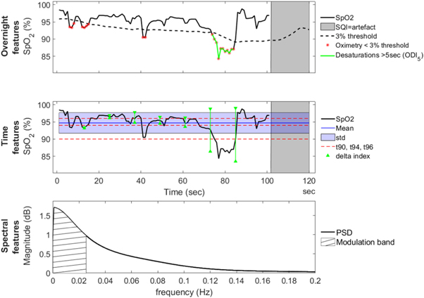
Figure 2. Example overview of a 2 min window recording of a subject, illustrating the different features extracted from the spO2 signal. Feature definitions are in table 2. The top figure shows part of the overnight signal to illustrate the overnight features ODI and SQI . The second figure shows a spO2 window with the extracted time features and the bottom figure shows the spectral domain and the corresponding power in the modulation band.
Download figure:
Standard image High-resolution imageTable 2. For each subject the spO2 features extracted from the spO2 signal were calculated in two ways: (1) overnight analysis, including signal quality percentage (SQP) and standard clinical ODI values and (2) the window-by-window analysis to extract time and spectral features. In each window, these time and spectral features were extracted and summarized by the mean, median, standard deviation and interquartile range over all windows of a night of a subject.
| Feature | Description | |
|---|---|---|
| Overnight analysis | ||
| Overnight | SQP
| The percentage of the night without artifacts. |
| ODI1, ODI5, ODI10 | This feature represents the amount of oxygen desaturations per hour of sleep with different durations, respectively lasting for at least 1 s, 5 s or 10 s. Were a desaturation is defined as a >3% decrease from the average in the preceding 120 s. | |
| Window-by-window analysis | ||
| Time | M | Mean of the spO2 signal. |
| std | Standard deviation of the spO2 signal. | |
| t90%, t94%, t96% | Cumulative time spent below 90%, 94% and 96% | |
| △-index | Quantifying SpO2 variability, computed as the average of absolute differences of the mean SpO2 between successive spO2 values sampled at 12 s intervals (Lévy et al 1996). | |
| Spectral | Pm | Power in the modulation frequency band (a frequency interval of 0.02 Hz centered around the modulation frequency peak, tracked in the band from 0.005 to 0.1 Hz). |
| Ptot | Total power. | |
| Pratio | Ratio between the power in the modulation frequency band and total power (Pm/Ptot). | |
For the overnight information, two general features were determined over the total night: the SQP , an indication of the portion of the signal containing no artifacts as determined by the SQI
 and the clinical feature ODI.
The window-by-window time features were extracted from each 2 min window. For the window-by-window spectral features, a power spectral density estimate using covariance method was applied to these 2 min spO2 windows to characterize the spO2 in the spectral domain and extract the spectral features. All time and spectral window-by-window features were described by their statistical distribution.
3.1.3. PPG characterization
Before further analysis, the PPG signal quality was evaluated using an SQIPPG algorithm (Karlen et al 2012). Each PPG signal segment is assigned a SQI between 0 and 100 based on a cross correlation method applied to an adaptive PPG cycle template and assumes that under non-artifact conditions each consecutive pulse is comparable and does not show much variation. The algorithm segments the PPG signal into pulses and makes use of the derivative of the PPG signal to find pulse slopes and an adaptive set of repeated Gaussian filters is used to select the correct slopes. For calculating the SQI, the similarity in the pulse shapes within a time frame are used and each new pulse is cross-correlated with the previous pulses to look for (irregular) signal morphology. Segments with low SQI (less than 50) will be automatically rejected from further analysis (Karlen et al 2012).
3.1.3.1. PPG features
Both the overnight and the window-by-window features of the PPG signal are summarized in table 3 and figure 3.
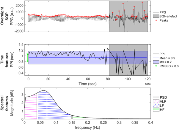
Figure 3. Example overview of a 2 min window recording of a subject, illustrating the different features extracted from the PPG and PPI signal. Feature definitions are table 3. The top figure shows the used PPG window with a red asterisk for each peak detection. The gray background indicates those parts where the signal quality is not good enough. The second figure shows the PPI signal extracted from the PPG signal, including the extracted time features. The bottom figure shows the spectral domain and the corresponding frequency bands.
Download figure:
Standard image High-resolution imageTable 3. For each subject the PPI and HRV features extracted from the PPG signal were calculated in two ways: (1) overnight PPG analysis included the SQPPPG and (2) the window-by-window analysis to extract HRV time and spectral features. In each window, these time and spectral features were extracted and summarized as the mean, median, standard deviation, and interquartile range over all windows of a night of a subject.
| Overnight analysis | ||
|---|---|---|
| Overnight analysis | ||
| SQPPPG | The percentage of the night without artifacts. | |
| Window by window analysis | ||
| Time | Mean of PPIs | The mean of PPIs |
| std of PPIs | The standard deviation of PPIs | |
| RMSSD | The root mean square of the successive differences between adjacent PPIs | |
| Spectral | VLF | Very low frequency band: 0.01–0.04 Hz |
| LF | Low frequency band: 0.04–0.15 Hz | |
| HF | High frequency band: 0.15–0.4 Hz | |
| Ptot | Total spectral power: 0.04–0.4 Hz | |
| nLF and nHF | Normalized powers of LF and HF: dividing both powers by the total spectral power. | |
| LF/HF ratio | The ratio of the low-to-high frequency power. | |
To estimate PRV from the PPG signal, the locations of the peak of pulses in the PPG were detected by using a zero-crossing algorithm to obtain the pulse to pulse interval (PPI)s for each window. The intervals between successive peaks were subsequently computed, and PPIs shorter than 0.33 s or longer than 1.5 s were considered as artifacts and deleted from the time series.
For the overnight information, one general feature was determined over the total night: the SQPPPG, calculated as the percentage of the recording with no artifacts. The overnight signal was cut into windows of 2 min to extract window-by-window features. The window-by-window time features were extracted from each artifact free 2 min PPI window (each window can only have a maximum duration of 50% containing artefacts, otherwise that specific 2 min window is excluded from further analysis). To extract the spectral features, the sequence of PPIs was first interpolated to create an uniformly spaced time signal with a sampling rate of 4 Hz, called the PPI signal. Secondly a power spectral density estimate using covariance method was applied on the interpolated PPI signal. The power of different frequency bands were computed by determining the area under the spectral density curve bounded by a specific bandwidth as described in table 3. All time and spectral window-by-window features were described by their statistical distribution.
3.2. Statistical analysis—NtN variability
Linear mixed models (LMM) were used to calculate the rate of variability between nights of each feature over time. This study first investigated whether features are significantly variable between nights (referred to as 'overall variability'), and whether the variability between nights was significantly different between both the OSA and the non OSA group (referred to as 'between groups variability'). If one of these showed significance, a post hoc analysis is performed to investigate whether this significance was specifically due to difference in location (home versus hospital) and the variability was compared among the two OSA severity groups (OSA versus nonOSA). Model residuals were checked to validate the assumptions underlying the LMM.
LMM were used to account separately for within-patient and between-patient variability using repeated measures per patient. In LMM models, the responses from a subject are thought to be the sum of both fixed and random effects. The LMM model included a random intercept by subject to account for between-subject differences and within subject correlation of observations and fixed effects for the night, the OSA severity, and the interaction between OSA severity and night. A standard mixed model for feature y, of subject i (i = 1, 2, 3,...,N subjects) on night j (j = 1, 2, 3 nights) is given as:

where Y is the response vector, X
β models the fixed effects, Z
γ the random effects and  is a vector of residual errors. With β and γ the vectors of the fixed and random effects parameters respectively. Observation matrices X and Z are the fixed effects and random effects variables respectively.
We fitted a mixed-effects model to investigate the variability for each feature. The fixed effects were the repeated night variable (night 1 (hosp) and night 2 and 3 (home)), the OSA severity (AHI>5 or AHI ≤ 5), and the interaction between OSA severity and night. A random effect parameter γ was added to model the subject variability denoted by Nr for each subject number.
Therefore, our model can be expressed as:

With either a significance in NtN variability and/or difference in NtN variability between groups. Additional calculations were made to describe (1) the mean and std of the parameters divided by group and location and (2) the p-value given for each group between overall NtN variability, hosp versus home or home versus home variability.
4. Results
4.1. Dataset
A detailed description of the number of recorded measurements considering the defined quality restriction for each night is given in figure 4 and the demographic information of the participants used in the analysis is provided in table 4. One patient withdrew from the study and 6 patients were excluded for not having good quality recordings longer than 3 h. In total we characterized the spO2 and PPG signals of 68 children (26 OSA and 42 nonOSA), of which 68 (100%) had at least 1 night, 59 (87%) with 2 nights, and 35 (51%) with three nights.
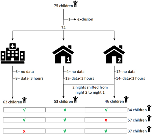
Figure 4. In the screen-my-sleep dataset, 75 children were recruited for PSG. One patient withdrew from the study, and the remaining 74 patients were asked for 3 nightly recordings with the PO; night 1 at the hospital simultaneously with PSG, and subsequently night 2 and night 3 at home. Data preparation consisted of removing the patients with no data or <3 h of recording time, and shifting measurements from night 2 to night 1 if the latter was missing. Respectively 63, 53 and 46 recordings were analyzed for the night at the hospital, first night at home and second night at home. A total of 34 (50%) children had a complete PO collection of three nights, 57 (84%) children had a night in the hospital and only 1 at home and 37 (54%) children had a missing night at the hospital but still had 2 measurements at home.
Download figure:
Standard image High-resolution imageTable 4. Demographic information of the included subjects in the dataset (mean ± std), * show a significant difference between both OSA and nOSA group evaluated by a t-test at p < 0.05.
| Total | OSA | nonOSA | p-value | |
|---|---|---|---|---|
| Clinical information | ||||
| Children (n) | 68 | 26 | 42 | |
| Male (Female) | 35 (33) | 10 (16) | 25 (17) | * |
| Age (std) | 8.3 (3.8) | 6.8 (3.9) | 9.2 (3.5) | |
| BMI (std) | 19.6 (5.9) | 18.6 (4.1) | 20.3 (6.8) | |
| PSG information | ||||
| AHI (std) | 6.0 (7.3) | 12.6 (8.1) | 1.9 (1.3) | * |
| TST (hours) | 6.7 (0.9) | 6.8 (0.6) | 6.6 (1.0) | |
| Sleep efficiency (%) | 83.2 (10.3) | 85.0 (7.0) | 82.0 (11.8) | |
| REM % | 18.5 (5.3) | 17.9 (6.5) | 18.9 (4.3) | |
| Awakenings (n) | 15.3 (12.8) | 17.6 (19.4) | 13.9 (5.6) | * |
| Respiratory events (n) | 18.5 (24.8) | 39.1 (30.0) | 5.8 (5.0) | * |
| ArousalIndex (%TST) | 2.9 (4.2) | 6.1 (5.4) | 0.9 (0.8) | * |
4.2. SpO2 characterization
Features extracted from recording with the PO were compared for NtN variability. An example overview of all spO2 signals of one patient recorded in the study can be seen in figure 5.
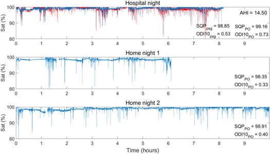
Figure 5. Example overview of raw SpO2 signals of a patient (AHI = 14.5) for three nights. The top figure shows the comparison between the SpO2 signals recorded during the hospital night with both PSG (red) and PO (blue), the bottom 2 figures show the two consecutive nights at home with only the PO. The overall SQP and ODI are given for comparison purpose.
Download figure:
Standard image High-resolution image
4.2.1. SpO2 variability
4.2.1.1. SpO2 overnight features.
Firstly, this study investigated whether spO2 overnight features were significantly variable between nights, or whether the overall variability was significantly different between the OSA and the nonOSA groups. Table 5 provides an overview of all spO2 overnight features (defined in the top row of table 2) with their corresponding p-value's. Almost all overnight spO2 features show no overall NtN variability in the recordings measured with the PO. Only the SQP shows a significant overall NtN variability between the three measured nights, with no significant difference of the between groups variability, in other words the NtN variability of the SQP
 is similar for both the OSA and the nonOSA group.
Table 5. All spO2 overnight features and their p-value in NtN variability. The middle column shows the significance in NtN variability of all subjects (nonOSA and OSA) and the right column shows whether this variability is significantly different between the nonOSA and OSA group. *shows significance p < 0.05.
| Overall | Between groups | |
|---|---|---|
| Features | NtN variability | NtN variability |
| ODI10 | 0.10 | 0.86 |
| ODI5 | 0.33 | 0.23 |
| ODI1 | 0.11 | 0.09 |
| SQP | <0.00* | 0.065 |
The SQP shows significant overall NtN variability and a post hoc analysis is performed to investigate whether this significance was specifically due to difference in location (home versus hospital) and the variability was compared among the two OSA severity groups. For the SQP
 this can be found in table 6. For the total population, there is a significant change in SQP over time [F(2,118) = 1.5, p = 0.00], explained by a higher SQP at the hospital during PSG than during the nights at home.
Table 6. Description of all spO2 features with either significant overall NtN variability or significant difference in NtN variability between groups. Providing the mean and standard deviation (mean (std)) of this feature of OSA and nonOSA over the three different nights recorded with the PO, one at the hospital and two at home. The p-values are determined using the linear mixed models and added to describe the NtN variability significance.
| PO | p-value | |||||||
|---|---|---|---|---|---|---|---|---|
| Hosp | Home | |||||||
| Features | Group | Hospital | Home1 | Home2 | Overall | versus | versus | |
| Home | Home | |||||||
| Overnight | SQP | total | 98.4 (4.1) | 94.2 (13.2) | 90.5 (17.6) | 0.00 | 0.02 | 0.04 |
| OSA | 97.9 (6.3) | 94.6 (12.2) | 96.2 (11.4) | 0.56 | 0.38 | 0.85 | ||
| nonOSA | 98.7 (1.9) | 93.9 (14.1) | 86.9 (20.0) | 0.00 | 0.03 | 0.02 | ||
| Time | std(t96) | total | 9.2 (12.5) | 16.5 (15.7) | 15.6 (14.3) | 0.00 | 0.004 | 0.96 |
| OSA | 13.3 (14.0) | 15.1 (18.1) | 11.0 (12.1) | 0.25 | 0.44 | 0.12 | ||
| nonOSA | 6.8 (11.0) | 15.4 (18.5) | 18.5 (14.9) | 0.00 | 0.00 | 0.27 | ||
It was also shown that the interaction between OSA and night was not significant at the 5% level (see right column in table 5), suggesting that the relationship of nights with SQP does not vary depending on OSA severity [F(2,116) = 3.1, p = 0.065]. However, further tests on the individual OSA severity groups, see the specific rows for OSA and nonOSA in table 6, showed no significant NtN variability in the OSA group, but significant NtN variability in the nonOSA group, with higher signal quality values reported in the night at the hospital compared to the nights at home.
4.2.1.2. spO2 time features
Similar to the overnight spO2 features, the NtN variability was also investigated for all spO2 time features mentioned in table 2, which were investigated by window-by-window analysis. First for the overall variability, although the mean, median and interquartile descriptions of all features showed no significant variability between the three nights, all standard deviations of the features showed a significant NtN variability. This variability was not significantly different between the nonOSA and OSA groups: however one feature the std of the cumulative time spent below 96% (std(t96)) showed a significant difference in the NtN variability between the groups.
Secondly, because the t96 showed significant NtN variability (F(2.109)=9.0, p = 0.00) and also a different variability within nights and between groups (F(2,108) = 4.0, p = 0.02), post hoc analyses can be found in table 6. The nonOSA group shows higher t96% values for the both nights at home compared to the night at the hospital, with overall no significant NtN variability (F(1,0.39) = 12.5, p = 0.41), but comparing the locations there is a clear NtN variability (F(1,34.7) = 12,67, p = 0.001). In the OSA group, the two nights at home show a different effect compared to the night at the hospital, resulting in a different type of variability.
4.2.1.3. spO2 frequency features
Also similar to the overnight spO2 features, the NtN variability was investigated for all spO2 frequency features mentioned in table 2, which where investigated by window-by-window analysis. All mean, standard deviation, median and interquartile descriptions of all features showed no significant overall variability nor between groups variability over the three nights.
4.3. PPG characterization
4.3.1. PRV overnight feature
Table 7 shows the detailed description of the SQPPPG over the three nights and the calculated significance regarding NtN variability. There is indeed a significant change in SQPPPG over time, and this table shows that the signal quality of the saturation signal is higher at the hospital during PSG then during the unsupervised nights at home.
Table 7. Description of all PRV features with either significant overall NtN variability or significant difference in NtN variability between groups. Providing the mean and standard deviation (mean (std)) of this feature of OSA and nonOSA over the three different nights recorded with the PO, one at the hospital and two at home. The p-values are determined using the linear mixed models and added to describe the NtN variability significance.
| PO | p-value | |||||||
|---|---|---|---|---|---|---|---|---|
| Hosp | Home | |||||||
| Features | Group | Hospital | Home1 | Home2 | Overall | versus | versus | |
| Home | Home | |||||||
| Overnight | SQP | total | 98.4 (4.1) | 94.2 (13.2) | 90.5 (17.6) | 0.00 | 0.02 | 0.04 |
| OSA | 97.9 (6.3) | 94.6 (12.2) | 96.2 (11.4) | 0.15 | 0.36 | 0.05 | ||
| nonOSA | 98.7 (1.9) | 93.9 (14.1) | 86.9 (20.0) | 0.29 | 0.40 | 0.25 | ||
| Time | M(stdRRI's) | total | 0.062 (0.030) | 0.056 (0.028) | 0.057 (0.028) | 0.00 | 0.43 | 0.01 |
| OSA | 0.053 (0.026) | 0.051 (0.031) | 0.056 (0.028) | 0.08 | 0.24 | 0.03 | ||
| nonOSA | 0.067 (0.030) | 0.060 (0.026) | 0.057 (0.028) | 0.06 | 0.34 | 0.12 | ||
| Spectral | M(LF) | total | 0.28 (0.28) | 0.20 (0.21) | 0.21 (0.26) | 0.04 | 0.48 | 0.05 |
| OSA | 0.22 (0.23) | 0.17 (0.17) | 0.20 (0.22) | 0.03 | 0.20 | 0.01 | ||
| nonOSA | 0.31 (0.30) | 0.23 (0.24) | 0.22 (0.28) | 0.13 | 0.50 | 0.07 | ||
| M(HF) | total | 1.75 (1.34) | 0.48 (0.36) | 1.2 (1.2) | 0.04 | 0.16 | 0.01 | |
| OSA | 1.43 (1.17) | 1.29 (0.10) | 1.93 (1.69) | 0.10 | 0.93 | 0.01 | ||
| nonOSA | 1.93 (0.41) | 0.61 (1.44) | 0.58 (1.30) | 0.10 | 0.15 | 0.04 | ||
4.3.2. PRV time features
Similar to the overnight PRV features, the NtN variability was also investigated for all PRV time features mentioned in table 3, which were investigated by window-by-window analysis. Both the IQR and std of the mean RRI's, and the median description of both RMSSD and the std RRI's, showed a significant variability between the three nights, but this variability was not significantly different between the nonOSA and OSA group.
A selection of these features are elaborated in table 7, providing the mean and standard deviation of these features between OSA, nonOSA and all subjects over the three different nights recorded with the PO.
4.3.3. PRV frequency features.
Also similar to the overnight PRV features, the NtN variability was also investigated for all PRV frequency features mentioned in table 3, which where investigated by window-by-window analysis. No features showed significant NtN variability, except for the median description of both the very low frequency power and the low frequency power, with no significant variability between the nonOSA and OSA group.
A selection of these features are elaborated in table 7, providing the mean and standard deviation of these features between OSA, nonOSA and all subjects over the three different nights recorded with the PO. All PRV frequency features show a significant NtN variability, regardless of the OSA severity group or location.
5. Discussion
In this article, we reported on the use of a portable pulse oximeter called the PO in children with suspicion of OSA, specifically the variability in measurements over different nights. This study used the SMS database consisting of 74 recordings in children, measured multiple nights with the PO, including one night simultaneously with PSG at the hospital and a minimum of two nights at home (Hoppenbrouwer et al 2018).
The measured variability in OSA features should help determine the reliability and minimal amount of diagnostic testing necessary to improve diagnostic accuracy using a portable pulse oximeter. The extracted features were investigated for possible NtN variability, with extra attention to the difference between nights at the hospital and at home. Given previous studies, we hypothesized at least a difference between both hospital and home, possibly from an adaptation response to a new location, the so called first night effect (FNE) (Agnew et al 1966, Sharpley et al 1988).
This study showed that most features do not have significant overnight differences and are relative constant between measurements measured during different nights. Future screening using such a portable pulse oximeter should take into account that some features could vary among nights, meaning that using these features in a screening model could cause a change in clinical classification. Therefore, when using these features, it may be useful to record more than one night of pulse oximetry data. The signal quality percentage (SQP) shows a higher NtN variability, especially comparing the night at the hospital with the nights at home. This can be explained by the unsupervised setting of at home measurements, possible leading to more movement artifacts compared to the hospital. However overall, the found variability between the multiple nights at home was not different compared to the variability found between measurements in hospital and at home.
This study contributes to the current literature on NtN variability. It helps to clarify previous findings, but also adds additional information by providing information between the difference between at home and at the hospital measurements.
The goal is for home pulse oximetry to help determine the minimal amount of diagnostic testing necessary to improve diagnostics accuracy, thereby reducing the PSG waiting list and OSA testing and make initial screening easier. The results of this study suggest that the feature extracted from portable pulse oximetry show relatively consistent values within the home environment. With smaller NtN variability, there is a greater confidence in the outcome of a measurement during one night. However in the case of larger NtN variability, this confidence is reduced and may increase the potential for misclassification of disease severity (Kryger et al 1996, Kapur et al 1999). Especially in patients with mild OSA, small changes in OSA variables due to NtN variability could decrease the severity classification under the diagnostic threshold.
NtN variability results across studies are discrepant. A possible explanation could be the difference in location and measurement techniques. Some studies investigate the variability of the AHI from PSG (Chediak et al 1996, Katz et al 2002, Stepnowsky et al 2004, Ahmadi et al 2009) and others only compared the spO2 features of portable at home testing (Pavone et al 2013, Burke et al 2016, Stöberl et al 2017), but none of these compared children with the same device both home and hospital measurements. Currently we use home screening to predict hospital outcome, but for that we should first know how the outcome of a portable device differs between those two locations.
This research not only focused on the understanding of the natural variability in measured sleep features at the same location, where most features show no significant NtN variability, but also investigated the difference between PSG and at home measurements. There is more variability between current measurement at the hospital and future at-home monitoring, which should be taken into account when comparing these outcomes. Another explanation between our results and other literature, is that most researches are looking at adults where we have included children.
Next to the normal NtN variances, one explanation of the difference between at home and at the hospital measurement could be the so called FNE. The FNE is a known effect in literature, stating that a nightly variability is due to the initial adaptation to the hospital and PSG environment (Agnew et al 1966, Bon et al 2000), but also that there could be a possibility that in lab PSG measurements can disrupt sleep and thereby overestimate the severity (Agnew et al 1966). This could suggest that differences in AHI are minimal and more representative of the real OSA severity when measurements are performed in a familiar environment. Indeed other studies investigating the variability of sleep features measured only at home showed a lack of FNE (Coates et al 1979, Sharpley et al 1988). Different papers have reported on this effect, mostly comparing the variability of the AHI or reporting the variability of specific variables, such as sleep quality variables (e.g. sleep stages, arousals, sleep efficiency). These papers describe that sleep quality variables that show a lack of this FNE when patients undergo sleep testing in an at-home environment (Coates et al 1979, Sharpley et al 1988), however more recent research has not always shown this effect, most likely due to the more comfortable setting of modern laboratories. Though this study did not focus on FNE specifically, it did show that the signal quality of a pulse oximetry signal contains more artifacts during the unsupervised nights at home. This means that at home testing should pay extra attention to those parts of the night that are noisy.
It's also worth discussing why some features show significant NtN variability, while other do not. Regarding the SQP feature, we expected to see a NtN variability based on the FNE mentioned above and these results are as expected. However interestingly enough, also the standard deviation of time spend below 96 showed a significant NtN variability. And even more interesting, this variability seems to be linked to the nonOSA group, for which we couldn't find an explanation in this study.
The discrepancy in previous literature can also be explained by difference in number of nights measured or the time between measurements. Most studies focused on the NtN variability of OSA across 2 nights, either consecutive (Fietze et al 2004, Stepnowsky et al 2004, Pavone et al 2013, Prasad et al 2016) or with a couple of weeks/months in between measurements (Katz et al 2002, Levendowski et al 2009b, 2009a, Stöberl et al 2017).
The focus of this study lies on whether each individual feature is changing over time, and thereby controlling for the variation coming from both nonOSA and OSA groups.
Another difficulty in comparing previous research are the different statistical analyses performed. When only comparing two nights, most studies use the standard student t-test, comparing the means of two samples relative to the standard error of the mean is limited to comparing only two nights at a time. The data of this study is divided over at least three nights and not all patients had the same amount of nights (unbalanced data), resulting in 'missing data' for some patients or the need to drop nights from the more complete patients. The repeated ANOVA is an extension of the dependent t-test for related, not independent groups; however, when taking missing data into account, LMM has a better ability to accommodate these types of unbalanced datasets. With LMM's not all individuals need to have the same number of observations at the same locations or at the exact same time points, reducing possible unnecessary removal of data. A suitable statistical test should also take into account intersubject differences, for which a repeated measure design is one of the most efficient methods. This makes sure that subjects are matched with themselves and between subject differences are taken into account to ensures the highest possible degree of equivalence across nights.
In reviewing the study results, it is also important to consider the limitations of this study. Our study population is moderate in size and consists of children suspected of having OSA. Whether these findings also apply to adults remains to be determined. Not only is this variability due to a difference in location, but we know from literature that the variability is also due to variation in physiological, pathological or other conditions (e.g. temperature, emotion, daily activity (Hall et al 2020) or alcohol intake (Issa and Sullivan 1982, Berry et al 1992, Izumi et al 2005)). During at home measurements no alteration or suggestions for sleep pattern such as sleep duration were encouraged. By doing so we tried to maintain the patients normal sleep patterns.
An additional limitation we can discuss is the distribution in gender. In this study, the number of males was significantly higher in the nonOSA group compared to the OSA group. From literature, we know that the physiological differences between men and women are noticeable in the cardiovascular health and thus in PPG waveforms However Vargas et al investigated the influence of gender in children on fluctuations in pulse oximetry and found no statistically significant difference regarding gender (Vargas et al 2008). However in this study we didn't focus on the influence of gender and therefore cannot exclude the potential influence of gender. Another discussion point, is the signal quality threshold. A threshold of 50% for signal quality was chosen in this study, however it's uncertain whether there is an influence of this threshold on the NtN variability.
Despite these limitations, this study findings support the prediction that at home monitoring with the PO reproduces comparable features compared to the measurement at the hospital.
The purpose for this study is future at home monitoring of children with sleep apnea. At home screening could reduce the PSG waiting list (Rotenberg et al 2010, Kao et al 2015, Watson 2016). In addition, a second advantage is that at-home measurements enables valuable progress tracking over time and enable multiple attempts at good quality data with much more limited costs and waiting lists compared to a full lab PSG.
This study suggests that most features measured with the PO show no significant variability between nights at home. The exact clinical significance should be investigated further.
Now that the variability of this device is better understood, future research can be focused on the prediction of the hospital outcome using the home measurements. Future research will focus on predicting OSA severity from home measurements and be compared with the PSG-based AHI outcome.
Most pulse oximetry features show no significant NtN variability and could be used in future at-home testing to create a reliable and consistent OSA screening tool.
Acknowledgments
The authors would like to thank the Pediatric Anesthesia Research Team and clinical staff of the sleep laboratory at the British Columbia Childrens Hospital for their efforts in data collection and continuing support.