

Abstract
Objective: A novel method for the imaging of static scenes using electrical impedance tomography (EIT) is reported with implementation and validation using numerical and phantom models. The technique is applicable to regions featuring symmetry in the normal case, asymmetry in the presence of a perturbation, and where there is a known, frequency-dependent change in the electrical conductivity of the materials in the region. Approach: The stroke diagnostic problem is used as a motivating sample application. The head is largely symmetrical across the sagittal plane. A haemorrhagic or ischaemic lesion located away from the sagittal plane will alter this natural symmetry, resulting in a symmetrical imbalance that can be detected using EIT. Specifically, application of EIT stimulation and measurement protocols at two distinct frequencies detects deviations in symmetry if an asymmetrically positioned lesion is present, with subsequent identification and localisation of the perturbation based on known frequency-dependent conductivity changes. Anatomically accurate computational models are used to demonstrate the feasibility of the proposed technique using different types, sizes, and locations of lesions with frequency-dependent (or independent) conductivity. Further, a realistic experimental head phantom is used to validate the technique using frequency-dependent perturbations emulating the key numerical simulations. Main results: Lesion presence, type, and location are detectable using this novel technique. Results are presented in the form of images and corresponding robust quantitative metrics. Better detection is achieved for larger lesions, those further from the sagittal plane, and when measurements have a higher signal-to-noise ratio. Significance: Bi-frequency symmetry difference EIT is an exciting new modality of EIT with the ability to detect deviations in the symmetry of a region that occur due to the presence of a lesion. Notably, this modality does not require a time change in the region and thus may be used in static scenarios such as stroke detection.
Export citation and abstract BibTeX RIS
1. Introduction
Electrical impedance tomography (EIT) is an emerging imaging technique with many applications including those in the biomedical, geophysical and industrial domains (Adler and Boyle 2017). The technique involves the placement of an electrode array around a body of interest with the injection of electrical current and measurement of voltage between electrode pairs according to a pre-defined stimulation-measurement 'protocol'. The complete set of measurements taken (a 'frame') can be used to generate an image of the electrical conductivity (σ) or permittivity of the interior of the body by solving a mathematical inverse problem. In this paper, we focus on EIT in the example biomedical application of stroke diagnosis. Biological tissues feature frequency-dependent conductivity (Brown 2003, Holder and Institute of Physics (Great Britain) 2005) and EIT in this context offers a relatively cheap, portable, non-invasive technique of imaging using hazard free low-frequency currents of low-amplitude (Hamilton 2017). However, EIT also has low spatial resolution with high sensitivity to noise, and electrode movement and contact (Brown 2003, Adler and Boyle 2017).
Therefore, EIT has found most success to date in applications that feature a time change in the region of interest, for example the monitoring of lung function (Adler and Boyle 2017). In such cases, images can be produced from differencing the 'before' and 'after' measurement frames with a degree of tolerance to errors, as any artefacts that appear in both frames are removed (Brown 2003, Adler and Boyle 2017). In other applications, there is no change in the region over time that can be exploited. For example, with acute stroke, the causative haemorrhagic or ischaemic lesion usually does not change significantly over the time period considered. In such static scenarios, applicable EIT modalities include absolute EIT (aEIT) and frequency difference EIT (fdEIT). The former is considered challenging (Adler and Boyle 2017, Hamilton 2017) while the latter, based on differencing measurement frames, each taken at different stimulation frequencies, offers some robustness to errors. However, fdEIT is not without challenges: it is sensitive to errors in modelling and instrumentation (Malone et al 2014a, 2014b, 2015).
Recently, we introduced symmetry difference EIT (sdEIT) as an approach to imaging challenging static scenes such as in stroke (McDermott et al 2018). The sdEIT technique was comprised of a two-step approach. The first step was detecting a deviation from normal symmetry if a unilateral lesion was present. This detection resulted in the imaging of the true lesion and a confounding anti-lesion of opposite conductivity in the mirror image position across the plane of symmetry. Then, in order to disambiguate between the true lesion and the confounding anti-lesion, the second step was to generate and analyse a pseudo time difference image using a simulated model of the normal. However, this second step requires an accurate model of the normal, and as such, this is a limitation of the sdEIT technique that may hinder its use in clinical applications.
Therefore, in this work, we propose an improved algorithm over that presented in (McDermott et al 2018), which we refer to as bi-frequency symmetry difference EIT (BFSD-EIT). Like sdEIT, the proposed technique comprises two steps; however, BFSD-EIT removes the need for a simulated model of the normal by instead using information from two different frequencies of measurement, combined with a priori information of the expected conductivity change in the tissues at the two selected frequency points. Unlike information on the head shape and size that is needed for sdEIT, a priori information on the tissue conductivities is available from the literature, albeit with an inherent degree of uncertainty in the quoted values (McDermott et al 2017). For this work, the conductivity values used are derived from studies specifically focused on the application of EIT to the stroke problem (Horesh 2006, Packham et al 2012, Avery et al 2017a). Furthermore, in this work, a 3D electrode layout is now used offering improved multi-dimensional information on the region of interest (Avery et al 2017a). At each step, 3D images and customised quantitative metrics are produced and analysed. The steps involved in BFSD-EIT are
- (i)detection of deviation from normal symmetry;
- (ii)disambiguation of lesion type.
The combined set of results of (i) and (ii) are used to identify the presence, type, and location of the lesion. Alternately, the results may also indicate the inability to detect a lesion.
The goal of this work is primarily to introduce the BFSD-EIT algorithm as a novel modality for tackling the imaging of static or quasi-static scenes. The BFSD-EIT technique is theoretically applicable to any region where there is a natural plane (or planes) of symmetry and where normal symmetry is disrupted by the presence of a perturbation (or indeed normal asymmetry is changed by a perturbation). In terms of biomedical applications this may include the neck, parts of the thorax or parts of the abdomen for uses such as the detection of unilateral lesions in the neck, lungs or kidneys. EIT is also applicable to non-biomedical applications such as those in the geophysical and industrial domains (Ismail et al 2005, Boyle 2016). In these areas, we envision BFSD-EIT being of value in, for example, assessing the contents of pipes at one cross sectional point or between different cross sections. However, for this work we have chosen the stroke diagnostic problem as a sample application for the development of the BFSD-EIT technique, exploiting the symmetry of the head across the sagittal plane.
Stroke is the loss of neurological function due to an interruption in blood flow with the aetiology being a haemorrhagic (bleed) or ischaemic (clot) lesion (Gomes and Wachsman 2013). A definitive diagnosis is required to initiate treatments that are radically dissimilar depending on which type of lesion is present (Bath 2000). For instance, tissue plasminogen activator (tPA) is used as a treatment for ischaemic stroke but may be fatal if given to a haemorrhagic stroke patient (Electronic Medicines Compendium and NICE (National Institute for Health and Care Excellence)). Diagnosis is currently by gold-standard imaging modalities including computed tomography (CT) and magnetic resonance imaging (MRI) (McDermott et al 2017). These provide images of quality and detail that EIT is unlikely to match, but they suffer from accessibility issues which is of acute importance in stroke patients where outcome is heavily correlated to commencement of prompt treatment (McDermott et al 2017, Powers et al 2018). The successful application of EIT to the stroke problem is by no means a trivial challenge (Holder and Institute of Physics (Great Britain) 2005, Horesh et al 2005). For this reason, we consider it a 'hard' problem but one where innovation is essential. There is an urgent need for a portable, low cost imaging system for this application that could be used by first responders to definitively diagnose the aetiology and hence commence treatment. EIT has the potential to meet this need, aided by (for example) the reduction of the problem (in the first instance) to that of 'bleed or clot'.
These two lesion types are more conductive (bleed) and less conductive (clot), respectively, than the surrounding brain tissue (Packham et al 2012). The two lesion types also differ in conductivity profiles with particular changes in conductivity seen in the low frequency range (particularly between 25 Hz and 100 Hz) (Packham et al 2012). Thus, frequency-dependent changes in conductivity can be taken advantage of to support the differentiation of the lesion type. Therefore, the BFSD-EIT algorithm is described in the numerical experiments through the sample application of stroke aetiology diagnosis. In the case of the phantom experiments, potato was used as a sample frequency dependent perturbation with a significant conductivity change in the range of operation (50–250 kHz) of the Swisstom EIT-Pioneer and Packham et al (2012).
The layout of the paper is as follows. The next section details the numerical models and experimental phantoms used to collect data. Then, in section 3, the proposed BFSD-EIT technique is described along with the resulting images and metrics. Section 4 reports results from numerical simulations with spherical bleed and clot lesions in a range of scenarios with differing sizes, locations, and signal-to-noise ratios (SNR) of the frames. For brevity, the complete images and metrics are not reported in full; instead, select metrics are reported to illustrate where the technique performs well and where it fails. In section 5, perturbations with frequency-dependent conductivity are examined in a variety of locations in a head-shaped tank phantom in order to validate the technique in a real-world situation (both with and without a skull layer). The significance and limitations of the proposed BFSD-EIT technique are discussed in section 6, and the paper is concluded in section 7.
2. Numerical models and experimental phantom
The anatomically realistic head model described in Avery et al (2017a) was the basis for the experiments of this study. This model was created from CT and MRI scans of an adult patient's head and is comprised of the tissues superior to a transverse plane along the level of inion-nasion line. In this model, 32 electrodes are positioned as described in Avery et al (2017a), resulting in four electrodes positioned along the sagittal plane and the remaining 28 forming 14 symmetric pairs across the plane of symmetry. A CAD model was produced in Autodesk Fusion 360, using the resources provided from Avery et al (2017a). For the work described in Avery et al (2017a), the model comprised of three layers with brain, skull and scalp layers. However, in this study, a cerebrospinal fluid (CSF) layer was added to the model, positioned between the skull and brain with a realistic thickness of 5 mm (Stokes et al 2005, Haeussinger et al 2011). This extra layer, resulting in a 4-layer model, is a more realistic representation of the anatomy of the head, inclusive of the resistive skull layer and conductive CSF layer surrounding the brain (Holder and Institute of Physics (Great Britain) 2005).
This 4-layer model was used in the numerical experiments. Lesions were modelled in the numerical simulations as spheres of volume 10 ml and 50 ml and were assigned conductivity values representative of either a bleed or clot. The volumes were selected as being representative of small and large volume lesions, with the median volume of intracerebral haemorrhages in the early stages of stroke reported as 17 ml (Fiebach et al 2004, Mobashsher et al 2016). Three distinct positions were chosen for the perturbations: Position I: in the centre of the brain; Position II: on the left side of the mid-height transverse plane towards the exterior of the brain; Position III: on the right side, below the mid-height transverse plane in a caudolateral position. These positions and lesion sizes, along with a computer aided design (CAD) model of the head including the electrode positions, are shown in figure 1. A finite element model (FEM) of the CAD model, comprised of 4158 375 elements with refinement around the electrode positions, was subsequently created from this CAD model using COMSOL (COMSOL Group). This FEM comprised the numerical model used in this work. The FEM is sectioned into four discrete layers: brain, CSF, skull and scalp. The numerical experiments modelled the stroke aetiology differentiation problem, with focus on the conductivity of tissues between 25–100 Hz. As such the scalp, brain and CSF layers were assigned realistic conductivities of 0.25 S m−1, 0.1 S m−1 and 2 S m−1 respectively (Horesh 2006), with the skull assigned a realistic conductivity distribution as a function of position ranging from 0.0069 S m−1 to 0.0129 S m−1 (Avery et al 2017a). These values are considered constant across this band (Horesh 2006, Avery et al 2017a). However, the bleed and clot lesions were assigned conductivity values dependent on the frequency points selected, as described later in sections 3 and 4. The spherical lesions with assigned conductivities could be readily added to the FEM, and measurement frames generated by forward solving of the FEM (Jehl et al 2015).
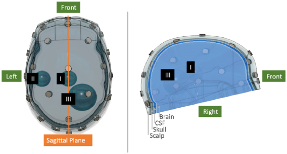
Figure 1. CAD model of the 4-layer head showing the scalp, skull, CSF and brain layers as well the position of the 32 electrodes. The sagittal plane represents a natural plane of symmetry in the head. Lesions in the numerical models were modelled as spheres of volume 10 ml and 50 ml positioned in one of positions I, II or III. In this figure, 10 ml lesions are shown at positions I and II, with a 50 ml lesion at position III. In the phantom, cubic phantoms of equivalent volume were used at the same locations.
Download figure:
Standard image High-resolution imageThe phantom was developed by 3D printing the adult tank described in Avery et al (2017a). The 3D print material was Accura® ClearVue™ polymer using a 3D stereolithography printer with a resolution of 4000 dots-per-inch (DPI). The resulting phantom is geometrically equivalent to the FEM numerical model, the exception being the absence of the CSF layer. The skull layer consists of pores designed to divide identical saline brain and scalp layers while allowing the flow of current in such a manner (presuming that saline of conductivity 0.4 S m−1 is used) that the effective conductivity of the skull is as modelled numerically. In the phantom experiments, perturbations were cubes of potato with either 10 cm3 or 50 cm3 volume, positioned as described above. Potatoes constitute a readily available material that exhibit frequency-dependent conductivity over the range of operation of the EIT hardware system used in this study, the Swisstom EIT-Pioneer and Packham et al (2012). The phantom is shown in figure 2 with electrodes attached and perturbation positioned. As is described in section 5, phantom experiments were conducted with both a 1-layer model with the skull removed, and a 3-layer model with the skull in place. In all cases, saline of conductivity of 0.4 S m−1 was used in the phantom experiments.

Figure 2. 3D printed phantom of the 3-layer head model with 10 ml potato perturbation at position III. The perturbations are suspended in place using a wooden pole and small stick as shown.
Download figure:
Standard image High-resolution imageThe proposed BFSD-EIT algorithm assumes symmetry about the sagittal plane. However the human head is not perfectly symmetric (Russo and Smith 2011, Kong et al 2018). As the head model used in this work (and particularly the boundary (scalp), skull and brain layers) are based on an actual human head, the model is also not perfectly symmetric. Table 1 provides a metric of the degree of symmetry of the four layers of the numerical model. The percentage of voxels of a given layer from the right-hand side (RHS) of the sagittal plane that if translated across the plane fall within the boundary of that same layer as delineated by the left-hand side (LHS) voxels is calculated. This calculation is repeated for the LHS translated onto the RHS, with the average of the two used to quantify the percentage overlap (a proxy for the degree of symmetry). Further, table 1 lists the distance error of the 32 electrodes as the distance between symmetric partners (if each electrode is translated across the sagittal plane onto the partner electrode). The electrode positions are selected largely from the electroencephalogram (EEG) 10–20 system (Avery et al 2017a) which should result in a high degree of symmetry (although are positioned on a realistic imperfectly symmetric scalp).
Table 1. Degree of asymmetry in the head model as (1) mean ± standard deviation of the distance errors of the 32 electrodes; (2) percentage overlap between the tissues from both sides.
| (1) | Mean (mm) ± standard deviation (mm) |
| Of distances between symmetric pair electrodes (if reflected across the sagittal plane) | |
| 0.08 ± 0.13 | |
| (2) | Percentage overlap |
| Of voxels of each respective tissue (if RHS reflected across the sagittal plane onto LHS and then vice-versa) | |
| Scalp | 93.5% |
| Skull | 90.1% |
| CSF | 90.9% |
| Brain | 98.3% |
3. Bi-frequency symmetry difference EIT
In this section, the BFSD-EIT technique is described in detail. The generation of both images and metrics, using the technique, is discussed step-by-step in section 3.1. Use-case examples, particularly of a 50 ml clot at position II in the numerical model is described in section 3.2.
3.1. BFSD-EIT algorithm and metrics
The algorithm can be summarised in two steps:
- (i)Detection of deviation from normal symmetry:The array of 32 electrodes on the scalp form 14 symmetric electrode pairs with the four electrodes on the sagittal plane forming symmetric pairs with themselves. A protocol is developed that maximises the distance between electrode pairs, leading to more channels that traverse the brain, supporting detection of both deep and superficial lesions (similar to the approach described in Malone et al (2014a)). A measurement frame is taken in this 'A-orientation' with a second frame taken in the mirror image 'B-orientation'. The B-orientation is made up of electrodes each of which is the symmetrical partner of the corresponding electrode in A-orientation. The protocol used in the same in both orientations.Data is collected with both orientations at frequency point 1, f 1, where the conductivity of the tissues is known as a priori information. A difference image is then produced using the frames from the two orientations, along with detection metrics. Deviations in symmetry between A-orientation and B-orientation are ideally detected. If a lesion is present on one side of the head, two objects will be detected: the lesion on the correct side of the head, and a confounding anti-lesion which has opposite conductivity and a mirror image position across the sagittal plane. If there is no lesion present, or if the lesion is positioned over the line of symmetry, no lesion will be detected.
- (ii)Disambiguation of lesion type:Step (i) is repeated at a new frequency point (frequency point 2, f 2). Ideally, the conductivity of the tissues at f 2 is known; however, at minimum the trend in the change of conductivity of the tissues with respect to the first frequency point should be known. The results of this step, in combination with the results of step (i) and the a priori knowledge of the trend in conductivity values between f 1 and f 2, can be used to disambiguate which type of lesion is the true pathology based on analysis of the images and the associated metrics.
These steps are also synopsised in figure 3.
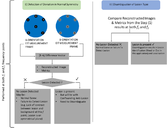
Figure 3. Summarised version of the two steps comprising the BFSD-EIT algorithm. In step (i), the outcome is the detection (or lack thereof) of a lesion. After step (ii), the conclusion is either no lesion detection or lesion detection with disambiguation resulting in identification (bleed or clot in this application) as well as localisation.
Download figure:
Standard image High-resolution imageFor stroke, the two lesion types are more (bleed) and less (clot) electrically conductive than the brain (Packham et al 2012). Hence after step (i) a bleed (if detected) would result in an image and metrics indicating the presence of a bleed with a confounding anti-lesion that is indistinguishable from a clot, and vice-versa. This inconclusive outcome necessitates step (ii) for disambiguation of lesion type.
Now that the technique has been described at a high level, the specifics are provided as follows. First, a protocol using a pair drive skip 0 pattern (Adler and Boyle 2017) is calculated which used the results from an inverse travelling salesman algorithm implemented using MATLAB and maximised distances between electrode pairs. Forward models of the numerical FEM with and without lesions (differing in conductivity, size, and location) were created. A measurement frame was generated for the A-orientation (arbitrarily assigned as the 'before' and denoted as FrameA). The protocol was repeated, and a frame was generated for the mirror image B-orientation (arbitrability assigned as the 'update' and denoted as FrameB). Each electrode in A-orientation and the corresponding electrode in B-orientation are symmetrical partners. In this way, a given measurement pair from a given orientation represents information on the mirror image scene to what is seen by the equivalent measurement pair of the other orientation. This symmetry between orientations is illustrated in figure 4.

Figure 4. Six electrodes from A-orientation and the symmetrically equivalent B-orientation are shown along with three sample electrode pairs from each orientation. Any given pair from A-orientation is the symmetric equivalent of that from B-orientation (for example A11–A12 is the equivalent of B11–B12). In the absence of a perturbation or if there is a perturbation lying on the sagittal plane, the measurement recorded from a given pair should be identical to the respective symmetric partner pair. In this diagram, a 50 ml perturbation is in position III (highlighted in blue). The perturbation will result in differences in the symmetric partner pair measurements. Also, it is seen that electrode #6 from both orientations lies on the plane of symmetry (the sagittal plane) and so is its own symmetric partner. Finally, it can be seen that the algorithm used to design the pair drive skip 0 pattern ensures that the distances between each electrodes pair constituting a channel is maximised.
Download figure:
Standard image High-resolution image0th ordered Tikhonov reconstruction onto a coarse mesh corresponding to A-orientation (252 705 voxels), using the difference vector (FrameB − FrameA) as an input. A given voxel will be of positive intensity (arbitrary units) if the difference vector indicates the measurements from B-orientation are more conductive than A-orientation at that location (with the size of the contribution of each measurement pair at that voxel dependent on the reconstruction algorithm) and negative if the measurements from B-orientation are less conductive than A-orientation at that location. The magnitude of the intensity is proportional to the magnitude of the difference, with each voxel having an individual intensity value. Quantitative metrics are produced from the set of voxel intensity values for each reconstruction from steps (i) and (ii). An image is also rendered.
The first metric calculated, the Global LHS and RHS Mean Intensity is calculated based on the intensity of the collective set of voxels of on each side of the sagittal plane. Subsequently, thresholding is performed to focus attention on regions of interest (ROI), which are candidate lesions, with further metrics applied to the detected ROIs.
- Global LHS and RHS mean intensity (GMI): The average intensity over all voxels on either side of the sagittal plane. In the presence of a lesion the values for RHS and LHS should be, ideally, of equal magnitude but opposite sign. In the absence of a lesion (or inability to detect a lesion), this 'equal but opposite' pattern will not be present and further, theoretically, the values in such cases should be near zero. This metric alone can be used to detect, identify and to an extent localise a lesion (as explained further in section 3). However, corroborative information from the images and other metrics is ideally also used before a diagnostic decision can be finalised.
Candidate lesions are then focussed on by thresholding to only show the highest and lowest 2% of voxels by intensity (value chosen empirically) to highlight contiguous ROIs. The ROIs are further filtered to remove ROIs < 5 ml in volume (deemed a threshold volume below which detection is unreliable) (Boverman et al 2016), and those centred within 10 mm of the mesh surface (deemed to be outside the brain layer and further, artefacts are often on the surface or around electrodes where EIT is sensitive to errors) (Stokes et al 2005, Adler et al 2015). The largest ROIs of both the high and low set of thresholded voxels are analysed (ROIH, ROIL) with further quantitative metrics including:
- Volume: The volume in cm3 of the ROI (i.e. the largest contiguous set of voxels in the thresholded image for both the ROIH and ROIL).
- Difference intensity per m3 (DIM): The intensity value (arbitrary units) of the ROI in the difference image per unit volume. Reported for both the ROIH and ROIL. The value is (+) for an increase in conductivity, (−) for a decrease. The trend in this metric for both ROIs should reflect that of the GMI.
- Difference in centroid location (DCL): The difference in the centroid locations between the ROIH and ROIL for a given image. If one ROI is reflected across the plane of symmetry, ideally the two ROIs should superimpose perfectly resulting in a DCL = 0. A large deviation from zero indicates that the two detected ROIs are not symmetric and there is no lesion present, or that the technique cannot detect the lesion. Therefore, this is the first metric that should be analysed after the GMI.
3.2. BFSD-EIT example cases
A numerical example is now presented, of a noise free case with a 50 ml clot at position III. The clot is assigned a conductivity of 0.05 S m−1 in step (i) (corresponding to a f 1 of 25 Hz) and then a conductivity of 0.09 S m−1 in step (ii) (corresponding to a f 2 of 100 Hz) (Horesh 2006, Packham et al 2012). As described in section 2, at these two frequency points, the other tissues (scalp, skull, CSF, brain) are considered to have constant conductivity. Reconstructed images at both frequency points, for the selected use-case example, are shown in figure 5. In this figure, voxels of intensity within the mean ± one standard deviation of the voxels constituting each ROI (ROIH and ROIL) are depicted. The figure hence is of the two ROIs and any other voxels with intensities within the high and low thresholded ranges. Figure 5 also provides the quantitative metrics associated with each frequency point.
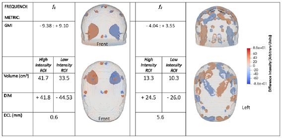
Figure 5. Reconstructed images and quantitative metrics for a 50 ml clot at position III. At f 1 the lesion has a conductivity of 0.05 S m−1 and the surrounding brain conductivity is 0.1 S m−1. The image for this frequency point shows ROIs suggestive of a conductive lesion in the true position and a confounding anti-lesion in the symmetrically opposite position. This result could be caused by a clot in position III or a bleed in the symmetrically opposite position. Also, artefacts are seen near the mesh surface. At f 2 a clot has a conductivity of 0.09 S m−1 while the brain conductivity is the same as at f 1. The result is a much noisier image at f 2 than f 1 due to the reduced contrast. A clot is expected to produce this behaviour while the image of bleed at f 2 would give a result identical to the first image (at f 1). Hence the true lesion must be a clot, at position III. The quantitative metrics support this conclusion with both the GMI and DIM having an 'equal but opposite' pattern with larger magnitude in figures at f 1 than at f 2 as a result of more contrast between the tissues at f 1 than at f 2. The enhanced contrast is also reflected in the increased volume of ROIs at f 1 and smaller DCL, relative to f 2.
Download figure:
Standard image High-resolution imageThe image at f 1 shows a conductive lesion in the correct position and a confounding non-conducting anti-lesion in the mirror image position across the sagittal plane. Artefacts are also present in the image, largely localised towards the surface of the mesh, which is especially sensitive to errors in electrode position (and in this case symmetry). Since the reconstruction is onto the mesh corresponding to A-orientation, the frame for A-orientation (the 'before') has embedded in it the information that a clot is at position III, with the rest of the scene normal. The frame for B-orientation (the 'update') indicates that the clot is in the mirror position to position III, and the rest of the scene is normal. Hence, the difference vector indicates that position III has changed from a non-conductive clot to normal (an increase in conductivity) while the mirror position has had the opposite change. This result could occur either due to a clot at position III or due to a bleed in the mirror image position. The image at f 2 indicates that the true lesion is that of a clot. This determination is evident from the images since at f 2 the image is noisier than at f 1 due to the decreased contrast between clot and brain conductivity at f 2 compared to at f 1. If the true lesion was a bleed, then the conductivity contrast between the bleed and the brain is the same at both frequency points and hence the images would be effectively identical. This conclusion is supported by the metrics. With the GMI metric, an overall increase in conductivity on the LHS is seen, and a near equal but opposite decrease occurs on the RHS. The magnitude of GMI values decrease at f 2 compared to f 1: this is expected behaviour for a clot on the LHS as the contrast between the lesion and surrounding brain decreases at f 2 relative to f 1. The ROI metrics correlate with a larger volume and DIM, with a smaller DCL, for the ROIs at f 1 compared to f 2 due to the improved contrast at f 1.
For completeness, additional results are shown in figure 6 that examine the three other possible scenarios that may occur. While in figure 5 the data corresponds to a scenario in which there is a clot on one side of the brain, in figure 6, the results demonstrate: a bleed on one side of the brain (10 ml bleed at position II), a bleed on the line of symmetry (50 ml bleed at position I), and for a normal brain (with no lesions).
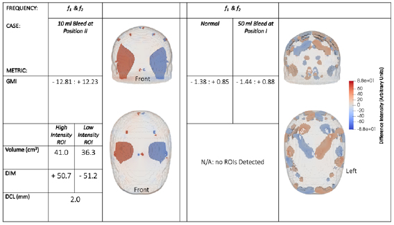
Figure 6. Reconstructed images and quantitative metrics for a 10 ml bleed at position II (left) and for a case where no lesion is present (right). For both scenarios, the conductivities of the tissues are the same at both f 1 and f 2, meaning the results are identical at both frequency points, hence only the results at one f point (arbitrarily f 1) are shown. The case with no lesion is near identical to the case where a 50 ml bleed is at position I (not shown), since there is no deviation in symmetry between the two sides when a lesion lies on the plane of symmetry and hence no lesion is detectable. Artefacts are seen near the mesh surface but are not part of the brain layer.
Download figure:
Standard image High-resolution imageA bleed is seen to give the opposite pattern of results to a clot; the reconstructed image of a bleed scenario has the ROIL in the true location. At the two chosen frequency points, the conductivity of a bleed and the surrounding brain tissue do not vary (0.7 S m−1 and 0.1 S m−1 respectively) hence, the two BFSD-EIT steps give identical results. Therefore, if the second step of the BFSD-EIT technique leads to results identical to those of the first step, then the lesion can be identified as a bleed. In the case of a normal, there is no difference in symmetry between the sides, and theoretically an image of low (near zero) voxel intensity is produced. Artefacts at or near the mesh surface in the scalp and skull layers are seen in the image and result in a non-zero GMI; however, the magnitude of this metric is much smaller than it would be if a lesion were present. The low magnitude of GMI means that more noisy voxels are visible as part of the 2% threshold; however, the image is clearly noise with no coherent ROI seen in the brain layer (the filters described in section 3.1 result in the artefacts not being detected as ROIs). The case of a lesion evenly positioned across the plane of symmetry gives the same result as a normal, as there is no deviation in the symmetry of both sides. Hence, even a large lesion such as a 50 ml bleed is undetectable using BFSD-EIT if it is positioned evenly across the line of symmetry.
4. Numerical simulations and results
In this section, the BFSD-EIT results are presented for the numerical simulations. In these simulations, the f 1 and f 2 values were chosen so that the conductivity of a clot changes from 0.05 S m−1 (corresponding to a f 1 of 25 Hz) to 0.09 S m−1 (corresponding to a f 2 of 100 Hz) while the conductivity values of scalp (0.25 S m−1), skull (0.0069 S m−1–0.0129 S m−1, varying spatially), CSF (2 S m−1), brain (0.1 S m−1) and bleed (0.7 S m−1) are constant between the two f values (Horesh 2006, Packham et al 2012, Avery et al 2017a). The rationale for the selection of the f 1 (25 Hz) and f 2 (100 Hz) values is the clear dichotomy in trend of conductivity values of bleed and clot with respect to the background tissues in this range, with this divergence necessary for BFSD-EIT (Packham et al 2012).
BFSD-EIT results from 13 cases are reported: a normal (i.e. healthy with no lesion), 10 ml and 50 ml lesions, of both bleed and clot, at each of positions I, II and III. The BFSD-EIT technique is applied to noise-free frames, and to frames with added noise at levels of 60 dB and 40 dB SNR. Due to the large size of the dataset, reporting of all results (images and metrics) from all scenarios is not possible; therefore, only the GMI, DIM, and DCL metrics are reported for brevity. Together, these metrics indicate when the technique works well and when it fails. However, we note that, ideally, a full set of results (with all images and metrics, as given in section 2), would be used for a firm conclusion to be reached regarding the presence, type, and location of a lesion. The notation for each case is described in table 2. This notation is used throughout with the addition of '1' or '2' added indicating a case at f 1 or f 2, respectively. Figure 7 shows the GMI results, while figure 8 gives the other quantitative metrics for various cases at the different noise levels.
Table 2. Notation for the numerical experimental setups (upper case—bleed; lower case—clot. Position I: centre of the brain; position II: left side of the mid-height traverse plane towards the exterior of the brain; position III: right side, below the mid-height traverse plane towards the exterior of the brain).
| Case notation | Case description |
|---|---|
| N | Normal (no lesion) |
| A/a | 10 ml, position I |
| B/b | 50 ml, position I |
| C/c | 10 ml, position II |
| D/d | 50 ml, position II |
| E/e | 10 ml, position III |
| F/f | 50 ml, position III |
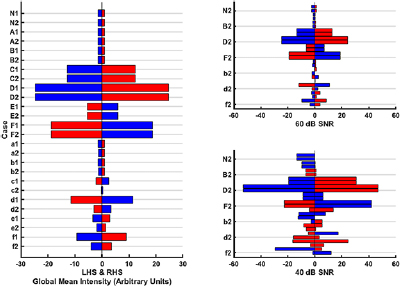
Figure 7. GMI metrics for each of the 13 cases at each of the noise levels. The notation used to describe each case is given in table 2 with '1' corresponding to f 1 and '2' corresponding to f 2. The blue bars represent a negative intensity value and the red bars a positive intensity value on either the LHS or RHS depending on the case. The normal case (N) and lesions on the sagittal plane (position I, i.e. cases A/a and B/b) are expected to have near zero values, bleeds away from the midline (positions II and III, i.e. cases C-F) are expected to give identical results at each frequency, and clots away from the midline (i.e. cases c–f) will result in values of increased magnitude at f 1 relative to at f 2 as the contrast between clot and the background reduces. Left: Results with noise-free frames (i.e. SNR = ∞). Right: Results with 60 dB and 40 dB SNR (note the axes correspond to those of the noise-free plot, with the grid lines grouping cases of the same location and nature). At 60 dB, the results are still similar, however now the 'equal but opposite' property is compromised. At 40 dB, results become excessively noisy with only cases C, D and F clearly detectable. These plots indicate that the presence and disambiguation of a lesion is possible with this metric alone. Larger lesions should have values of greater magnitude than the corresponding smaller lesion. The localisation, to the level of whether the lesion is in the LHS or RHS, is also possible to derive. For example, case 'f ' is a 50 ml clot at position III (the same as in figure 5). The LHS value is negative, and the RHS positive. As described in section 2, after disambiguation as a clot based on the difference in values between f 1 and f 2, this pattern of LHS and RHS values must be due to the lesion being on the LHS. A bleed of the same volume and in the same location (assuming away from the sagittal plane) to a clot gives a larger magnitude of intensity at f 1 (or f 2) as the contrast between bleed (0.7 S m−1) and brain (0.1 S m−1) is always larger than between clot (0.05 S m−1 at f 1, 0.09 S m−1 at f 2) and brain. Finally lesions nearer the exterior give larger magnitude values than the same lesion deeper in (consider D/d compared with F/f).
Download figure:
Standard image High-resolution image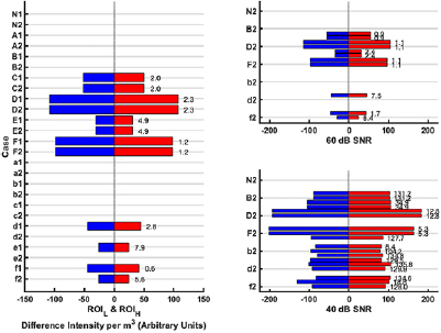
Figure 8. The quantitative ROI metrics: DMI and DCL for the 13 cases at various noise levels. If no ROI is detected in a given case at a given frequency point, then no metric value is listed. Left: The noise-free scenario (i.e. SNR = ∞). Right: The results at 60 dB and 40 dB SNR levels (note the axes correspond to those of the noise-free plot, with the grid lines grouping cases of the same location and nature). The bars represent the DMI for the ROIH (red bar) and ROIL (blue bar). The DCL between a ROIH and ROIL for a given case is reported in mm to the right of the red bar. Ideally, DCL = 0; therefore, cases with high values indicate failed detection.
Download figure:
Standard image High-resolution imageThe GMI metric alone can detect, identify, and to an extent localise a lesion. Alternatively, this metric can indicate that there is no lesion or that there is a failure to detect a lesion. In figure 7, the GMI values should, as a first feature, have theoretically 'equal but opposite' values regardless of the case. The normal case and cases with the lesion at position I (A–B, a–b) are seen to give near zero values, indicating that both sides are symmetrically balanced and hence no lesion is present, or the lesion cannot be detected as it lies on the plane of symmetry. For those lesions in positions II (C–D, c–d) and III (E–F, e–f), the values of the mean intensities should deviate away from zero with larger values seen for larger lesions; this is the case with the 10 ml lesion giving smaller mean intensities compared to the corresponding 50 ml lesion at the same location. A bleed will give identical results at both f 1 and f 2 while a clot (which has a larger contrast compared to the background at f 1 relative to f 2) will result in a larger magnitude intensity metric at f 1 compared to f 2. These trends between f 1 and f 2, which can be seen in figure 7 can be used to disambiguate a bleed from a clot. Finally, the side that the lesion is on can be derived from the mean intensities. For example, for the 50 ml clot at position III (case 'f'), the LHS mean intensity is negative and the RHS mean intensity metric positive (as explained in section 3). A clot on the opposite side (for example, in case 'd') will have the opposite pattern. For measurement frames where noise is added, it is seen that the algorithm performs well at 60 dB, with excessive degradation in performance at 40 dB SNR (only cases C, D and F are detectable at this noise level). Notably, a bleed of the same volume and location as a clot (if away from the sagittal plane) always gives a larger magnitude of intensity as the contrast between bleed/brain is larger than that of clot/brain at f 1 and f 2. Finally, lesions nearer the extremity give larger magnitude values than the equivalent lesion deeper in the brain (consider D/d (nearer the exterior) compared with F/f (deeper in and nearer the sagittal plane)).
ROIs are detected in the noise-free reconstructions for the position II and III cases C–F. No ROIs are detected as expected for the normal or position I cases (N, A–B, a–b), with only artefacts/noise presenting in the images of the latter set as seen in figure 6, right. Further, only the case f has a ROI detected at both f 1 and f 2 with cases d–e only detected at the higher contrast f 1; implying the ROI detection is less sensitive to lesions than the GMI metric. However, it is noted that the detection of the clot at f 1 and failure to detect at f 2 may be sufficient to disambiguate the lesion as a clot as the expected trend of conductivity change is followed (the expected reduction in contrast at f 2 leads to failure to detect). Quantitative metrics are applied to the cases where ROIs are detected. The DMI metric gives results and pattern similar to those of the GMI metric: equal but opposite values, larger for bigger lesions (compare C versus D; E versus F), larger for lesions nearer the exterior (compare C versus E; D versus F). The DCL metric, ideally zero for symmetric ROIs, is less than 6 mm in all cases where a lesion is detected except for the sole case of a 10 ml clot detected (case e1). The results at 60 dB are similar with the exception of case e1 now not being detected. At 40 dB, cases D and F give reasonable results but with excessive noise present (evidenced by the often excessively large DCL and violation of the equal but opposite principle). Clearly better detection is achieved with a higher SNR. Some EIT applications, for example thoracic functional monitoring, can be successfully performed with systems offering an SNR of 30–40 dB (Wi et al 2014). However, more challenging applications, including those involving the head, usually require higher SNRs (Wi et al 2014) with hardware capable of circa 80 dB available including the ScouseTom system (Avery et al 2017b).
5. Phantom experiments
This section reports the application of the BFSD-EIT technique to an experimental scenario using an anatomically realistic 3D printed tank model of the head and skull, of identical geometry to the numerical model used in previous sections (but without a CSF layer), with frequency-dependent perturbations.
A full description of the head phantom is given in section 2 (Avery et al 2017a). All experiments were performed with both a 1-layer model with the skull removed, and a 3-layer model with the skull in place. In all cases, saline of conductivity of 0.4 S m−1 was used. A Swisstom EIT-Pioneer system was connected to the 32 electrodes used (Swisstom EIT-pioneer set). Before use, the system was allowed to warm up for 1 h. The injection protocol followed the same pair drive skip 0 pattern used in the numerical simulations. Potato cubes were used as frequency-dependent perturbations, with cubes of volume 10 cm3 and 50 cm3.
As described in Packham et al (2012), potato represents a frequency-dependent material with a measurable change in conductivity occurring over the kHz range (Packham et al 2012), in the operating range of the Swisstom EIT-Pioneer. Measurements were taken at 80 kHz (f 1) and 100 kHz (f 2), capturing two frequencies across which potato features a significant increase in conductivity with respect to the saline background. Potato was found to be conductive with respect to the background at both f points, with enhanced contrast at f 2 compared to f 1.
These cubes were placed in positions I, II and position III. The potato cubes were placed in the saline for an hour before taking recordings in order to ensure equilibration (Packham et al 2012). Then, measurements were taken for both A-orientation and B-orientations with the recordings were of 1 min duration, taken at 10 frames per second, and averaged, for each perturbation size, position, and when no perturbation was present (normal case), at both f 1 and f 2. The SNR of the hardware setup was calculated from the frames as the ratio of the mean to the standard deviation of the values for each measurement channel, then averaged for all channels across all frames at both frequency points. Using this method, the SNR was determined to be approximately 50 dB.
The BFSD-EIT method was applied, and results generated as in the previous sections. The results are reported in the same style as section 4; the GMI metric results are given in figure 9 with the DIM and DCL metrics shown in figure 10. The notation used for the phantom experiments is given in table 3 (again with the addition of '1' or '2' added indicating a case at f 1 or f 2 respectively). Sample reconstructed images of case 'F' for the 1-layer and 3-layer cases at both f points are shown in figure 11. It is again emphasised that a complete set of images and metrics is ideally used to assess a case but for brevity not all images are shown in this paper.
Table 3. Notation for the phantom experiments (position I: centre of the brain; position II: left side of the mid-height traverse plane towards the exterior of the brain; position III: right side, below the mid-height traverse plane towards the exterior of the brain).
| Case notation | Case description |
|---|---|
| N | Normal (no perturbation) |
| A | 10 cm3, position I |
| B | 50 cm3, position I |
| C | 10 cm3, position II |
| D | 50 cm3, position II |
| E | 10 cm3, position III |
| F | 50 cm3, position III |
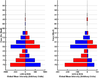
Figure 9. GMI results for each of the seven cases with the 1-layer phantom (left) and 3-layer phantom (right). The notation used to describe each case is given in table 3 with '1' corresponding to f 1 and '2' corresponding to f 2. The blue bars represent a negative intensity value and the red bars a positive intensity value on either the LHS or RHS depending on the case. The potato perturbation is conductive with respect to the saline background at both f 1 and f 2, with increased contrast expected at f 2. The normal case (N) and perturbations on the sagittal plane (position I, i.e. cases A and B) are expected to have near zero values. Position II and III cases (C–F) are expected to result in a negative intensity on the side the perturbation is truly on (with an equal but opposite positive intensity on the other side) and with the magnitude of intensities increasing from f 1 to f 2. The smaller perturbation will follow the same pattern as the larger perturbation in a given location but result in smaller magnitude of values (C compared to D; E compared to F). Finally, perturbations nearer the exterior (C and D) will give higher magnitude values compared to those further from the exterior (E and F). These expected patterns are borne out for the no skull (1-layer) set of results. A priori knowledge of the expected pattern of conductivity change for potato with respect to saline (and knowledge of other perturbation types and the associated conductivity patterns that may exist) allows the detection, identification, and to an extent localisation of the perturbation as potato. In the case of the 3-layer phantom (with skull) the presence of the skull which is a highly insulating layer dampens the signal, indicated with the lower magnitude of values compared to the 1-layer case. The results are as expected for cases D–F but the 'equal but opposite' principle is violated.
Download figure:
Standard image High-resolution image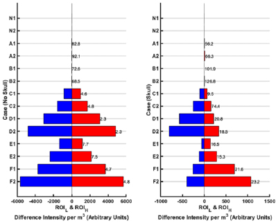
Figure 10. The quantitative ROI metrics: DIM and DCL for the seven cases with the 1-layer phantom (left) and 3-layer phantom (right). If no ROI is detected in a given case at a given frequency point, then no metric value is listed. The bars represent the DIM for the ROIH (red bar) and ROIL (blue bar). The DCL between the ROIH and ROIL for a given case is reported in mm to the right of the red bar. The results indicate that lesions are detectable, with expected behaviour, when no skull is present; however, detection suffers using these metrics when the skull is present.
Download figure:
Standard image High-resolution image
Figure 11. Reconstructed images for a 50 cm3 cubic potato perturbation at position III in the 1-layer phantom case (left) and the 3-layer case with the skull (right). The images at both 80 kHz (f 1) and 100 kHz (f 2) are shown. Potato is found to become more conductive with respect to saline from f 1 to f 2 with the enhanced contrast at f 2 evidenced by sharper ROIs and more intense ROIs at this point. The skull layer, being highly insulating, reduces the signal rendering images noisier when compared to the simpler 1-layer case. Further, the intensity of the voxels of the ROIs in the skull case is lower than in the no skull case.
Download figure:
Standard image High-resolution image
The GMI metric for the 1-layer phantom case correlates with the results from the numerical simulations. The normal (N) and cases with the perturbations at position I (A–B) give near zero results at both f points indicating no lesion is present or the inability to detect a lesion. For the other cases where the perturbations are away from the sagittal plane, the 'equal but opposite' rule is generally followed; larger perturbations in the same location give larger magnitude results than smaller perturbations at a given f (C versus D; E versus F); perturbations nearer the exterior result in larger magnitude values than equivalent lesions nearer the sagittal plane (C versus E; D versus F). Potato is conductive with respect to saline at f 1 with this contrast enhanced at f 2. This change results in the greater magnitude of GMI values for a detected case at f 2 compared to f 1 (which allows identification of the perturbation as truly being potato), Finally, the perturbation being conductive will result in a negative intensity on the side it is located with confounding positive intensity on the opposite side at a given f (as explained in section 3). A priori knowledge of the expected pattern of conductivity change at the two selected f points of the materials involved (saline, potato in this case) allows disambiguation of the material as being potato. Hence, detection, identification and localisation on the left or right is demonstrated. With the skull, the signal is dampened as evidenced by the lower magnitude of intensities. The results are as expected for cases D–F but the 'equal but opposite' principle is violated.
ROIs detection in the 1-layer case gives results analogous to the GMI results. ROIs are detected for cases A and B but the low DIM values, high DCL values (>70 mm), as well as the images, should identify these as cases where no perturbation is detectable. For cases C–F, the 'equal but opposite' principle applies; smaller perturbations give results of lower magnitude of DMI compared to the corresponding larger perturbation; perturbations nearer the exterior are better detected than those nearer the sagittal plane (evidenced here by the lower DCL of C versus E; D versus F). The magnitude of DIM is larger for the f 2 result compared to f 1 as expected by the higher contrast at f 2. For the skull cases, the trend of results seen in the metrics remains the same as for the corresponding 1-layer cases but violation of the 'equal but opposite' principle, a lower magnitude of DIM, and an increase in the value of DCL are indicative of the challenge posed by the insulating skull layer.
The images of case F correlate with the metrics. The 1-layer model results in a sharper, less noisy and higher magnitude of intensity values for the detected ROIs compared to the 3-layer case. In both the 1-layer and 3-layer scenarios, the intensity of the ROIs at f 2 are more intense compared to that of f 1 as expected by the enhanced contrast between potato and saline at f 2.
Overall, the experimental results have demonstrated the proof-of-concept for using BFSD-EIT on symmetric regions with conductivity changes across frequency, as illustrated here with a realistic head-shaped tank.
6. Discussion
This work explores a novel EIT modality to facilitate imaging of scenarios that are static in nature. A range of scenarios fall into this category including important biomedical applications such as stroke diagnosis, where the identification of the aetiology as bleed or clot is vital. The BFSD-EIT technique is based on the selection of a frequency point (f 1) where a priori information on the conductivity of the tissues of interest, and the conductivity contrast between possible pathological tissue and normal background parenchyma, is available. Next, detection of deviations in symmetry across a natural symmetrical plane in the area of interest is performed by comparing EIT measurements from mirror image electrode pairs, and then reconstructing an image and calculating quantitative metrics based on the image. The image and metrics indicate detection of a lesion, as well as a confounding anti-lesion of opposite conductivity. Alternatively, no lesion may be detected indicating a normal scene or an inability of the technique to detect a lesion. In order to disambiguate a detected lesion from the anti-lesion, the technique is repeated at a 2nd frequency point (f 2) with again a priori information on the conductivity and contrast between the tissues. Analysis of the results from both steps—both images and associated metrics, leads to either detection, identification, and localisation of the lesion, or a conclusion that no lesion is present (or detectable). Stroke is an excellent sample application to demonstrate BFSD-EIT as the two aetiologies are effectively opposite in conductivity to each other with respect to the background. However, other conditions may only have one aetiology or aetiologies that do not have this conductivity profile. In these cases, the elaborate disambiguation process is redundant. A final result may be interpreted from some key metrics alone, in particular the GMI metric and for the detected ROIH and ROIL: DIM and DCL; but ideally the aggregate collective of images and metrics should be used to reach a firm conclusion.
Care must be taken in the selection of f 1 and f 2. The trend in conductivity changes of the tissues at the two selected frequency points should be such that the contrast between the differing confounding perturbations and the background at f 1 and f 2 display a different pattern of change in order to achieve disambiguation. In the case of stroke, values of f 1 and f 2 that allow disambiguation are documented as described in section 4 (f 1 of 25 Hz, f 2 of 100 Hz), where the contrast between blood and brain is constant at the two frequency points whereas the contrast between clot and brain decreases from f 1 to f 2.
This study demonstrates the feasibility and effectiveness of the BFSD-EIT technique in a variety of numerical and experimental scenarios using anatomically accurate models of the head. In the numerical models, a 4-layer head model is used in the implementation of BFSD-EIT with spherical bleeds and clots at a variety of different locations, at two volumes (10 ml and 50 ml), with realistic conductivity values at a variety of SNR levels. These models demonstrate the effectiveness and limitations of the technique. Detection of lesions is stronger with higher SNRs, larger lesion sizes, and lesions nearer the exterior (away from the plane of symmetry). In clinical applications, the use of these f points would result in further technical challenges particularly in terms of the maximal current amplitude allowed, which is 100 µA RMS (141 µA peak) at frequencies below 1 kHz as set out in the IEC 60601-1 guidelines (International Electrotechnical Commission 2002). However, robust EIT data has been collected from stroke patients at these frequencies (Goren et al 2018), supporting the potential feasibility of the algorithm in real world scenarios given the appropriate hardware, such as the ScouseTom (Avery et al 2017b) used in Goren et al (2018).
The technique was also validated experimentally in a 1-layer and 3-layer phantom model (without and with a skull layer) using 10 cm3 and 50 cm3 cubic perturbations of a material (potato) that has a significant increase in conductivity from 80 kHz (f 1) to 100 kHz (f 2) which is within the frequency range of the Swisstom EIT-Pioneer. These perturbations were detected against a saline background with, as per the numerical models, detection, identification and localisation possible. Detection with the phantom skull in place was, as expected, more challenging than without. The selection of this experimental setup was driven by the relatively easy commercial availability of the Swisstom EIT-Pioneer system, opposed to for example the ScouseTom, and the significant change in the conductivity of (again easily available) potato in the operating range (Packham et al 2012). This hardware would not however be suitable for clinical application to the stroke problem as the range of operation (50 kHz–250 kHz) is outside that of where significant change in tissue conductivity is seen (Horesh 2006, Packham et al 2012). Further, the SNR (calculated as approximately 50 dB) would not be suitable for head applications (Wi et al 2014). Importantly, the BFSD-EIT algorithm is not dependent on a particular frequency per se but rather on there being a detectable conductivity change in the tissues or materials at the two selected frequency points. For the phantom setup this conductivity change was in the range 80 kHz–100 kHz while for the numerical setup the significant change was in the range 25 Hz–100 Hz. It is emphasised that the goal of this study is primarily the introduction of the BFSD-EIT algorithm with feasibility of clinical application of the technique envisioned in subsequent work following this study.
BFSD-EIT represents an iterative, but substantial, improvement over the recently introduced sdEIT. The use of two frequency points removes the need for an accurate numerical model of the normal scene to disambiguate lesion types. Further, this work has advanced upon sdEIT through the usage of a 3D electrode layout and has introduced more robust metrics. However, like sdEIT, BFSD-EIT has an absolute limitation due to the technique being based on detecting deviations in symmetry between two sides of a body separated by a natural plane of symmetry. Hence, it can only be used in cases where the presence of lesion(s) alone results in an asymmetry. This technique cannot be used where there are symmetrically balanced bilateral lesions or where the background does not feature symmetry in the normal case. Symmetry is an inherent requirement for the algorithm, but the model used in the study is anatomically accurate and derived from a real patient with a real-world amount of asymmetry in the tissue layers and also in the electrode positioning as shown in table 1. However, future studies will be needed to assess the sensitivity of the technique to errors in modelling including deviations in the symmetrical placement of electrodes, deviations in the symmetry of the anatomy in the normal scene, and the assumed identical nature of partner electrodes. A further challenge for future work will be to assess the effect of a background with frequency-dependent conductivity. Finally, accurate and precise tissue conductivity values are a source of active research with inherent variability in literature values due to numerous factors such as the natural heterogeneity in tissues, heterogeneity between people and the measurement technique used (Electronic Medicines Compendium). The result is a band of uncertainty around assumed a priori values. While the trend in conductivity changes between f points is more important to BFSD-EIT, the analysis at a given f point does leverage these assumed values. This assumption that the conductivity values are accurate is a problem faced by all EIT modalities. The extent to which the BFSD-EIT algorithm is robust to deviations from the assumed conductivity values of tissues also remains to be assessed. Some of these are challenges shared and relevant to techniques for imaging static scenes such as fdEIT, while others (particularly those related to symmetry) are pertinent to BFSD-EIT.
The emphasis of this study is the introduction and description of the BFSD-EIT algorithm with successful application to stroke not the immediate focus. However, in the specific context of application of the technique to the stroke diagnostic problem and particularly moving from numerical models to more realistic phantom stroke models or indeed clinical scenarios the hardware setup as used in this study would not be suitable. As stated above the f points of interest in bleed and clot detection are outside the frequency range of the Swisstom EIT-Pioneer system with additional limitations including the low SNR offered by the system as well as a minimal current of 1 mA peak (Swisstom EIT-pioneer set). The clinical data gathered in Goren et al (2018) was recorded at frequencies ranging from 5 to 2000 Hz (covering the f points of interest for stroke) and within IEC 60601-1 guidelines. While the study of Goren et al (2018) reported an average SNR of 50 dB (with a maximum of about 56 dB), the work of Avery et al (2017b) analysed the same data finding that noise from cabling and current sources were significant issues lowering the SNR. This finding suggests that hardware optimisation for stroke application is feasible with other strategies for maximising SNR including taking advantage of the static nature of the pathology to allow averaging of sequential measurements.
7. Conclusions
EIT is a promising technology proposed for imaging in a variety of biomedical and other applications. However, EIT imaging generally struggles with scenes that are effectively static throughout the timeframe of interest. Existing EIT modalities (aEIT and fdEIT in particular) that attempt to image static scenes have challenges that hamper the efficacy of these modalities. BFSD-EIT represents an important step forward in the use of EIT to detect lesions in such scenarios. This technique is capable of detecting lesions where the presence of the lesion disrupts a normally symmetrical scene. BFSD-EIT identifies and quantifies these disruptions in symmetry through comparison of mirror image EIT measurement channels, subsequent reconstruction of an image, and analysis of metrics based on the image. This process is performed twice, at two carefully selected frequency points (which result in known and differing trends in conductivity changes between the tissues comprising the pathology and the background). The aggregate images and metrics result in disambiguation of the true lesion from a confounding anti-lesion. In the case of stroke, this disambiguation is essential as a bleed and a clot have similar magnitude of conductivity contrast with respect to the background brain tissue, but with opposite sign.
BFSD-EIT is seen to perform best for larger lesions, those further from the plane of symmetry and where there is a relatively high SNR, with the results shown here indicating hardware offering >60 dB SNR needed for robust detection (with respect to the sample stroke diagnostic application). We believe BFSD-EIT to be an exciting addition to the field of EIT and one that will catalyse the application of the technology into a range of important biomedical (and other) applications, including stroke.
Acknowledgments
The research leading to these results has received funding from the European Research Council under the European Union's Horizon 2020 Programme/ERC Grant Agreement BioElecPro n.637780, Science Foundation Ireland (SFI) grant number 15/ERCS/3276, the Hardiman Research Scholarship from NUIG, the charity RESPECT and the People Programme (Marie Curie Actions) of the European Union's Seventh Framework Programme (FP7/2007–2013) under REA Grant Agreement no. PCOFUND-GA-2013-608728. James Avery was supported by the NIHR Imperial BRC.
Appendix. Hardware and software resources
All models and software relating to the tank model is available at https://github.com/ EIT-team/Tanks (archived at DOI:10.5281/zenodo.1489106). The forward solver used, PEITS (Parallel EIT Solver) is available at https://github.com/EIT-team/PEITS (archived at DOI: 10.5281/zenodo.1641128), and the reconstruction software is available at https://github.com/EIT-team/Reconstruction (archived at DOI: 10.5281/zenodo.1643416).