

Abstract
Objective: We exploited a model-based Wiener–Granger causality method in the information domain for the evaluation of the transfer entropy (TE) and interaction TE (ITE), the latter taken as a measure of the net balance between redundancy and synergy, to describe the interactions between the spontaneous variability of heart period (HP) and systolic arterial pressure (SAP) and the effect of respiration (R) on both variables. Approach: Cardiac control was typified via the genuine TE from SAP to HP, that from R to HP, and the ITE from SAP and R to HP, while vascular control was characterized via the genuine TE from HP to SAP, that from R to SAP, and the ITE from HP and R to SAP. The approach was applied to study age-related modifications of cardiac and vascular controls in a cohort of 100 healthy humans (age from 21 to 70 years, 54 males) recorded at supine rest (REST) and during active standing (STAND). A surrogate approach was exploited to test the significance of the computed quantities. Main results: Trends of the genuine information transfer with age, already present in literature, were here confirmed. We originally found that: (i) at REST redundancy was predominant over synergy in both vascular and cardiac controls; (ii) the predominance of redundancy of the cardiac control was not affected by postural challenge, while STAND reduced redundancy of vascular control; (iii) the net redundancy of the cardiac control at REST gradually decreased with age, while that of vascular control remained stable; (iv) during STAND net redundancy of both cardiac and vascular controls was stable with age. Significance: The study confirms the relevance of computing genuine information transfer in cardiovascular control analysis and stresses the importance of evaluating the ITE to quantify the degree of redundancy of physiological mechanisms operating to maintain cardiovascular homeostasis.
Export citation and abstract BibTeX RIS
1. Introduction
Spontaneous oscillations of cardiovascular variables, visible in humans over beat-by-beat recordings of few minutes, are the manifest consequence of the simultaneous and incessant action of huge variety of short-term regulatory mechanisms aiming at maintaining variables within a physiological range of values according to a homeostatic principle (Cohen and Taylor 2002). Short-term control mechanisms can be classified as neural (e.g. autonomic nervous system influences (Pagani et al 1997, Marchi et al 2016a)) versus non-neural (e.g. Frank-Starling law and mechanical effects of respiratory-related modifications of intrathoracic pressure on venous return and stroke volume (Baselli et al 1994, Caiani et al 2000, Elstad and Walloe 2015)), as self-sustained (e.g. vasomotor centers in the brainstem (Guyenet 2006)) versus reflex (e.g. cardiac and sympathetic baroreflex (De Boer et al 1987, Marchi et al 2016b)), as central (e.g. respiratory centers in the brainstem (Eckberg 2003, Dick et al 2009)) versus peripheral (e.g. peripheral vasomotion (Nilsson and Aalkjaer 2003, Baselli et al 2006). All these mechanisms operate during the entire life of the organism but exhibit an evolution with age (Lakatta 1993). Indeed, aging alters cardiovascular control by modifying the relative importance of influences (e.g. sympathetic control increases with age (Kelly and O'Malley 1984, Seals and Esler 2000), while vagal one decreases (Laitinen et al 2004, Beckers et al 2006)), by reducing the effectiveness of some reflexes (e.g. cardiac baroreflex sensitivity is reduced during senescence (Parker Jones et al 2003)), by depressing the activity of self-sustained oscillators (e.g. the cardiac pacemaker activity (Larson et al 2013)), by diminishing the responsiveness of receptors and/or systems to inputs (e.g. sinus node responsiveness to sympathetic outflow (Lakatta 1993)) and by introducing instabilities (e.g. the cardiorespiratory interactions become less stable (Iatsenko et al 2013)). All these effects have been carefully documented via the assessment of the magnitude of the input–output relation between two variables. However, recent applications of tools based on information processing have expended the possibility of characterizing an input-output relation above and beyond the classical description in terms of transfer function towards the assessment of the genuine ability of an input to reduce the uncertainty of the output, namely the information transfer computed via transfer entropy (TE) (Hlavackova-Schindler et al 2007, Barnett et al 2009, Wibral et al 2011, Porta and Faes 2016b). Some seminal cardiovascular control studies have explored the effect of senescence on the information transfer in cardiovascular control. Nemati et al (2013) suggested that the ability of respiration (R) to reduce the uncertainty about future variations of heart period (HP) decreases with age and this finding was taken as an indication of a progressive decrease of the cardiorespiratory coupling with age. Porta et al (2014) found that the genuine ability of HP to reduce the unpredictability of systolic arterial pressure (SAP) decreases with age and this finding was taken as an indication of the progressively increased exploitation of the mechanical properties of the cardiac muscle compared to other mechanisms of SAP regulation (e.g. the diastolic runoff). Very few studies assessed the evolution of information transfer in cardiovascular control with age and, remarkably, no study monitors more peculiar portions of the information transfer assessing synergy, as the extra information transfer occurring when all inputs are jointly observed instead of separately, and redundancy, as the information transfer shared by all the inputs (Stramaglia et al 2012, Barrett 2015, Faes et al 2015, Porta et al 2015a). These quantities appear to be particularly appealing when the target is the characterization of the cardiovascular control and its evolution with age. Indeed, given the myriad of regulatory mechanisms targeting directly and indirectly the same physiological variable and the impact of senescence on the interactions among distinct reflexes, markers of redundancy/synergy are expected to change with age and provide a characterization of the impact of senescence on cardiovascular control complementary to those based on the magnitude of the input–output relation.
The aim of this study is to monitor the evolution of indexes measuring the redundant/synergistic contribution of vasculo-respiratory interactions to cardiac control and of cardio-respiratory interactions to vascular control with age. This monitoring was carried out by computing the interaction TE (ITE) from SAP and R to HP and from HP and R to SAP in a cohort of 100 healthy subjects with age ranging from 21 to 70 years (20 individuals in each ten years wide bin) recorded at rest in supine position (REST) and during sympathetic activation induced by active standing (STAND) (Catai et al 2014, Porta et al 2014). The computation of ITE markers is accompanied by the computation of the genuine information transferred from SAP and R to HP and from HP and R to SAP (Porta et al 2015b).
2. Model-based TE and ITE
The model-based approach to the evaluation of TE and ITE is based on the description of the dynamic of the target signal in a full universe of knowledge accounting for all interacting signals and its comparison with a more limited description of the same dynamic obtained in a restricted universe of knowledge excluding one or more driving signals. In this specific application three time series with zero mean and unit variance y = {y(n), n = 1,...,N}, u1 = {u1(n), n = 1,...,N} and u2 = {u2(n), n = 1,...,N}, where n is the progressive counter and N is the series length, form the full universe of knowledge Ω = {y, u1, u2}, while the restricted Ωs were obtained from the full Ω by excluding one of the source series, Ω\u2 = {y, u1} and Ω\u2 = {y, u1}, or both, Ω\u1u2 = { y }. Under the hypothesis of Gaussianity, the actions of u1 and u2 on y are jointly described in the full Ω via an autoregressive model with two exogenous inputs u1 and u2 (Söderström and Stoica 1989, Baselli et al 1997). More specifically, the current value of y, y(n), depends on p past samples of the same signal, y(n − k) with k = 1, ..., p, through the autoregressive portion of the model, and on p + 1 − τ1 past samples of u1, u1(n − k − 1 − τ1) with k = 1,..., p + 1 − τ1, and on p + 1 − τ2 past samples of u2, u2(n − k − 1 − τ2) with k = 1,...,p + 1 − τ2, through the two exogenous portions of the model. The description of the dynamic of y in the restricted Ωs is based on the same class of models exploited in the full Ω but one of the two exogenous parts (i.e. the block from u2 to y in Ω\u2 and that from u1 to y in Ω\u1) or both (i.e. the blocks from u1 and u2 to y in Ω\u1u2) are missing. Regardless of the type of Ω (i.e. full or restricted) the coefficients of the autoregressive and exogenous (if present) portions of the model can be estimated via traditional least squares approach and Cholesky decomposition method (Söderström and Stoica 1989, Baselli et al 1997), the model order can be optimized via the extension of the Akaike figure of merit to multivariate processes (Akaike 1974) and the delay of the action from u1 and u2 to y (i.e. τ1 and τ2) can be a priori decided according to physiological considerations and measurement conventions (Baselli et al 1994, Porta et al 2013). After solving the identification problem comprising the estimation of the coefficients, optimization of the model order and a priori setting of the latency of the exogenous influences on the destination, the one-step-ahead prediction of y(n) can be simply obtained by multiplying the values of y, u1 and u2 with the estimated coefficients according to the model structure (Porta et al 2013). Defined the prediction error as the difference between y(n) and its one-step-ahead prediction, the variances of the prediction error in Ω,  , in Ω\u2,
  , in Ω\u1,
  , and in Ω\u1u2,
  , measure the inability of the model in fitting the target dynamic in each Ωs. The variances of the prediction error range between 0 and the variance of y (i.e. 1) indicating perfect and null prediction respectively. According to Barnett et al (2009) the conditional joint TE (CJTE) from u1 and u2 to y given u2 measuring the uncertainty about y(n) that can be resolved from the knowledge of u1 above and beyond that can be resolved from u2 and past values of y (i.e. the genuine information transfer from u1 to y) is given by

Analogously, the CJTE from u1 and u2 to y given u1 quantifies the genuine information transfer from u2 to y as

According to Porta et al (2015b) the joint TE (JTE) from u1 and u2 to y measuring the uncertainty about y(n) that can be resolved from the knowledge of u1 and u2 above and beyond that can be resolved from past values of y (i.e. the total information transfer from u1 and u2 to y) is given by

Some studies suggest that the net synergy/redundancy of u1 and u2 in fixing the future behavior of y can be assessed via the functional, referred to as ITE (Stramaglia et al 2012, Barrett 2015, Faes et al 2015, Porta et al 2015a), defined as

 indicates redundancy of u1 and u2 to fix the future behavior of y if it is larger than 0 because conditioning for an exogenous source reduces the information transfer from the other to the destination. Conversely, if
  synergy is detected because conditioning for an exogenous source, usually termed as suppressor, improves information transfer from the other to the destination. Equivalently,
  can be computed as

where

and

measure the information transfer from u1 to y and from u2 to y respectively when u1 and u2 are considered separately (i.e. in Ω\u2 and Ω\u1). The (5) provides the most frequently utilized formalization of the net balance between synergy and redundancy (Timme et al 2014): i.e. redundancy is observed when the sum of the information transferred from u1 and u2, when the two source signals are considered separately, is larger than the information transfer when they are jointly considered, while synergy occurs when the joint observation of both inputs leads to an extra information transfer compared to their separated observation.
3. Experimental protocol and data analysis
3.1. Experimental protocol
Data belong to an historical database collected to evaluate the evolution of the cardiovascular control complexity and its response to a sympathetic stressor with age (Catai et al 2014, Porta et al 2014). Therefore, we refer to Catai et al (2014) and Porta et al (2014) for the full description of the protocol. Recording sessions were carried out at the Department of Physiotherapy of the Federal University of São Carlos, São Carlos, Brazil. The study was performed according to the Declaration of Helsinki for medical research involving humans and approved by the Human Research Ethics Committee of the Federal University of São Carlos (protocol number 173/2011). A written informed consent was obtained from all subjects.
Briefly, 100 subjects (aged from 21 to 70, 54 men) were studied (Porta et al 2014) and divided into five groups (20 subjects for each group), according the age ranges: 21–30; 31–40; 41–50; 51–60; 61–70. All subjects were apparently healthy, took no medicine influencing cardiovascular system, had no history and no clinical evidence of any disease based on clinical and physical examinations. Smokers, habitual drinkers and obeses (body mass index larger than 30 kg m−2) were excluded from this study. Only women without contraceptive medication or hormone replacement therapy were included. All women in 51–60 and 61–70 were in the menopausal phase. All subjects were evaluated in the afternoon in a temperature- and humidity-controlled room. Subjects were instructed to avoid caffeinated and alcoholic beverages as well as strenuous exercises during the day before the experiment. They were also instructed to ingest a light meal at least 2 h prior to the test. The subjects were maintained at REST for 10 min before starting recording. Then, signals were acquired for 15 min at REST and during STAND. STAND session followed always the REST one. The subjects were instructed to breathe spontaneously but they were not allowed to talk. All subjects completed STAND without experiencing any sign of pre-syncope.
The electrocardiogram (ECG) from a modified lead I, continuous plethysmographic arterial pressure (Finometer PRO, Finapress Medical System, The Netherlands) and respiratory movements via thoracic belt (Marazza, Monza, Italy) were digitalized using a commercial device (Power Lab 8/35, ADInstruments, Australia). Signals were sampled at 400 Hz. The arterial pressure was measured from the middle finger of the left hand being maintained at the level of heart by fixing the subject's arm to his/her thorax. The auto-calibration procedure of the device was switched off after the first automatic calibration at the onset of the protocol.
3.2. Beat-to-beat series extraction
The series of HP, SAP and sampled R were extracted from ECG, arterial pressure and respiratory movement signals respectively. After detecting the QRS complex on the ECG and locating its peak using parabolic interpolation, HP was approximated as the temporal distance between two consecutive parabolic apexes. The maximum of arterial pressure inside of the nth HP (i.e. HP(n)) was taken as the nth SAP (i.e. SAP(n)). Respiratory movement signal was sampled once per cardiac beat at the occurrence of the first QRS complex delimiting HP(n), thus obtaining the nth R measure (i.e. R(n)). HP(n), SAP(n) and R(n) were expressed in ms, mmHg and arbitrary units (a.u.) respectively. The detection of the QRS complexes and SAP peaks were carefully checked to avoid erroneous detections or missed beats. After computing HP(n), SAP(n) and R(n), sequences of 256 consecutive measures were randomly selected inside REST and STAND periods (Task Force 1996). The series were first linearly detrended and, then, the null hypothesis of restricted weak stationarity was tested (Magagnin et al 2011). If nonstationarities, such as very slow drifting of the mean or sudden changes of the variance, were detected according to (Magagnin et al 2011), the random selection inside the session of analysis (i.e. REST or STAND) was carried out again until the null hypothesis of restricted weak stationarity was accepted. The procedure was performed automatically by the software of the analysis.
3.3. Surrogate data
The significance of the computed indexes was tested against a situation of full uncoupling between the two exogenous sources and the destination. In order to destroy only the causal interactions from u1 to y and from u2 to y, while preserving as much as possible the other statistical properties such as distribution, power spectrum and self-entropy of all considered signals, surrogate data are generated by time shifting u1 and u2 according to a randomly chosen delay much larger than the maximal order of the model (i.e. 50 cardiac beats). The original sequence of y was kept untouched (Andrzejak et al 2003, Porta et al 2015b). For each original triplet of HP, SAP and R sequence we generated one triplet of surrogate series. The values at the end of the u1 and u2 were wrapped to their onset.
3.4. Calculation of the information-theoretic indexes
Assigned HP as the effect variable and SAP and R as the two exogenous causes, we computed the genuine information transfer from SAP to HP (i.e.  ) and from R to HP (i.e.
  ) and the interaction information transfer from SAP and R to HP (i.e.
  ) and, assigned SAP as the effect variable and HP and R as the two exogenous causes, we computed the genuine information transfer from HP to SAP (i.e.
  ) and from R to SAP (i.e.
  ) and the interaction information transfer from HP and R to SAP (i.e.
  ). Fast vagal actions of the cardiac baroreflex and cardiopulmonary reflexes were accounted for by setting the delays of influences from SAP and R to HP to 0 and 0 beats respectively (Eckberg 1976, Porta et al 2013). The delay from HP to SAP was set to 1 beat according to the measurement conventions imposing that HP(n) cannot affect SAP(n) because HP(n) was not ended yet when SAP(n) was taken (Baselli et al 1994). Immediate effects of respiratory-related changes of the intrathoracic pressure on SAP via modulation of the venous return and stroke volume were accounted for by setting the delay from R to SAP to 0 beats (Baselli et al 1994, Porta et al 2013). The model order p was optimized in the range from 8 to 14 over the most complex model structure identified in the full Ω. The whiteness of the prediction error and its mutual uncorrelation, even at zero lag, with the two exogenous series was checked over the same model (Baselli et al 1997). The model structures in the restricted Ωs were separately identified from the data using the optimal model order estimated in Ω. Indexes were computed over the original series and surrogates. Identification procedure and optimization of the model order over surrogate data was completely independent from that of the original series.
3.5. Statistical analysis
After pooling together all subjects regardless of the age two-way repeated measures analysis of variance (Holm–Sidak test for multiple comparisons) was applied to test the difference between experimental conditions assigned the type of series (i.e. original or surrogate series) and between original and surrogate series assigned the experimental condition (i.e. REST or STAND). Linear regression analysis of  ,
,  ,
,  ,
,  ,
,  and
and  on age was carried out over original data and surrogates. Pearson product moment correlation was calculated. Statistical analysis was carried out using a commercial statistical program (Sigmaplot, ver. 11, Systat Software, San Jose, CA, USA). A p < 0.05 was always considered as significant.
4. Results
Figure 1 shows examples of HP, SAP and R recorded in an healthy 22 year-old subject (figures 1(a), (b) and (d)) and in an healthy 68 year-old individual (figures 1(f), (g) and (i)) respectively. While HP mean is similar in the two subjects (i.e. 907 versus 823 ms), HP variance is higher in the young subject than in the old individual (i.e. 3355 versus 456 ms2) and SAP mean and, more evidently, SAP variance are smaller (i.e. 103 versus 123 mmHg and 35 versus 77 mmHg2). Examples of surrogate series are shown as well (figures 1(c) and (e) and figures 1(h) and (j)). When the target series is HP, SAP and R surrogates were obtained by time shifting the original SAP and R series with a delay longer than 50 beats (here the randomly chosen delays were 51, 55, 59 and 58 beats in figures 1(c), (e), (h) and (j)).  ,
,  and
and  computed over the original series are 0.114, 0.089 and 0.134 respectively in the young subject (figures 1(a), (b) and (d)), while they are 0.103, 0.096 and 0.047 in the old individual (figures 1(f), (g) and (i)).
  ,
,  and
and  computed over the surrogates are 0.016, 0.013 and −0.002 respectively in the young subject (figures 1(a), (c) and (e)), while they are 0.021, 0.014 and 0.010 in the old individual (figures 1(f), (h) and (j)).
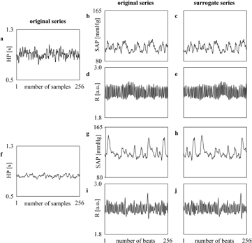
Figure 1. Examples of HP, SAP and R series derived from an healthy 22 year-old subject ((a), (b) and (d)) and from an healthy 68 year-old individual ((f), (g) and (i)) are shown. When the target series is HP, surrogate data ((c), (e), (h) and (j) respectively) are obtained by time shifting the original SAP and R series with a random delay longer than 50 beats (i.e. 51, 55, 59 and 58 beats respectively), while the original HP variabilities ((a) and (f)) are left unmodified.
Download figure:
Standard image High-resolution imageFigure 2 shows the grouped error bars of  (figure 2(a)),
  (figure 2(b)) and
  (figure 2(c)) computed over the original series (black bars) and surrogates (white bars) as a function of the experimental condition (i.e. REST and STAND). The subjects were pooled together regardless of the age and indexes were reported as mean plus standard deviation. Over the original series
  increased significantly during STAND (figure 2(a)), while
  significantly decreased (figure 2(b)). Conversely,
  (figure 2(c)) was not affected by the postural change. No significant between-condition differences were observed when the indexes were computed over surrogates. Assigned the experimental condition (i.e. REST or STAND)
  ,
,  and
and  computed over the original data were significantly larger than the corresponding quantity computed over surrogates (figures 2(a)–(c)). The percentage of subjects with
  < 0 was 4% and 5% at REST and during STAND respectively, while these percentages increased to 61% and 61% in surrogates.

Figure 2. The grouped error bar graphs show  (a),
(a),  (b) and
  (c) computed over original data (black bars) and surrogates (white bars) as a function of the experimental condition (i.e. REST and STAND). Values are pooled together regardless of age and reported as mean plus standard deviation. The symbol # indicates a significant change between original and surrogate data within the same experimental condition (i.e. REST or STAND), while the symbol * indicates a significant modification between experimental conditions within the same type of data (i.e. original series or surrogates) with p < 0.05.
Download figure:
Standard image High-resolution imageFigure 3 shows the simple scatters of the individual values (open circles) of  (figures 3(a) and (d)),
  (figures 3(b) and (e)) and
  (figures 3(c) and (f)) on age at REST. Values were computed over the original data (figures 3(a)–(c)) and surrogates (figures 3(d)–(f)). The linear regression (solid line) and its 95% percent confidence interval (dotted lines) are plotted when the slope of the regression line is significantly different from 0. When computed over the original data
  (figure 3(c)) was significantly associated with age and the correlation coefficient r was negative (r = − 0.255, p = 1.04 × 10⁻²), while
  (figure 3(a)) and
  (figure 3(b)) were unrelated to age (r = −0.048, p = 6.32 × 10⁻¹ and r = 0.030, p = 7.69 × 10⁻¹ respectively). When computed over the surrogate data
  (figure 3(d)),
  (figure 3(e)) and
  (figure 3(f)) were stable with age (r = −0.072, p = 4.75 × 10⁻¹, r = 0.014, p = 8.89 × 10⁻¹ and r = 0.012, p = 9.08 × 10⁻¹ respectively).

Figure 3. The simple scatters show the individual values (open circles) of  ((a) and (d)),
  ((b) and (e)) and
  ((c) and (f)) on age at REST. The values are computed over the original ((a)–(c)) and surrogate ((d)–(f)) data. When the slope of the regression line is significantly different from 0, the linear regression (solid line) and its 95% confidence interval (dotted lines) are plotted as well. A significant negative correlation of
  on age is detected only over the original data.
Download figure:
Standard image High-resolution imageFigure 4 has the same structure as figure 3 and shows the same quantities in the same position. At difference with figure 3,  (figures 4(a) and (d)),
  (figures 4(b) and (e)) and
  (figures 4(c) and (f)) were computed during STAND. When computed over the original data
  (figure 4(a)),
  (figure 4(b)) and
  (figure 4(c)) was unrelated to age (r = −0.176, p = 7.94 × 10⁻², r = 0.027, p = 7.91 × 10⁻¹ and r = −0.154, p = 1.27 × 10⁻¹ respectively). This finding was confirmed over the surrogate data (r = −0.069, p = 4.94 × 10⁻¹, r = −0.116, p = 2.52 × 10⁻¹ and r = 0.180, p = 7.34 × 10⁻² respectively, figures 4(d)–(f)).

Figure 4. The simple scatters show the individual values (open circles) of  ((a) and (d)),
  ((b) and (e)) and
  ((c) and (f)) on age during STAND. The values are computed over the original ((a)–(c)) and surrogate ((d)–(f)) data. When the slope of the regression line is significantly different from 0, the linear regression (solid line) and its 95% confidence interval (dotted lines) are plotted as well. No significant association of the reported information-theoretic indexes with age was found.
Download figure:
Standard image High-resolution imageFigure 5 shows examples of SAP, HP and R recorded in an healthy 28 year-old subject (figures 5(a), (b) and (d)) and in an healthy 68 year-old individual (figures 5(f), (g) and (i)) respectively. Similarly to figure 1 HP and SAP means are similar in the two subjects (i.e. 1060 versus 1110 ms and 124 versus 127 mmHg), HP variance is larger in the young individual than in the old subject (i.e. 1693 versus 814 ms2) and SAP variance is smaller (i.e. 7 versus 81 mmHg2). Examples of surrogate series are shown as well (figures 5(c) and (e) and figures 5(h) and (j)). When the target series is SAP, HP and R surrogates were obtained by time shifting the original HP and R series with a randomly chosen delay longer than 50 beats (here the random delays were 57, 52, 63 and 54 beats in figures 5(c), (e), (h) and (j)).  ,
,  and
and  computed over the original series are 0.172, 0.419 and 0.139 respectively in the young subject (figures 5(a), (b) and (d)), while they are 0.102, 0.299 and 0.113 in the old individual (figures 5(f), (g) and (i)).
  ,
,  and
and  computed over the surrogates are 0.014, 0.017 and −0.005 respectively in the young subject (figures 5(a), (c) and (e)), while they are 0.008, 0.019 and 0.001 in the old individual (figures 5(f), (h) and (j)).

Figure 5. Examples of SAP, HP and R series derived from an healthy 28 year-old subject ((a), (b) and (d)) and from an healthy 68 year-old individual ((f), (g) and (i)) are shown. When the target series is SAP, surrogate data ((c), (e), (h) and (j) respectively) are obtained by time shifting the original HP and R series with a random delay longer than 50 beats (i.e. 57, 52, 63 and 54 beats respectively), while the original SAP variabilities ((a) and (f)) are left unmodified.
Download figure:
Standard image High-resolution imageFigure 6 shows the grouped error bars of  (figure 6(a)),
  (figure 6(b)) and
  (figure 6(c)) computed over the original series (black bars) and surrogates (white bars) as a function of the experimental condition (i.e. REST and STAND). The subjects were pooled together regardless of the age and indexes were reported as mean plus standard deviation. In the original series postural modification did not change
  (figure 6(a)) and
  (figure 6(b)). Conversely,
  (figure 6(c)) significantly decreased during STAND. When the indexes were computed over surrogates, no significant between-condition differences were observed. Assigned the experimental condition (i.e. REST or STAND),
  ,
,  and
and  computed over the original data were significantly larger than the corresponding quantities computed over surrogates (figures 6(a)–(c)). The percentage of subjects with
  < 0 was 9% and 17% at REST and during STAND respectively, while these percentages increased to 59% and 67% in surrogates.

Figure 6. The grouped error bar graphs show  (a),
(a),  (b) and
  (c) computed over original data (black bars) and surrogates (white bars) as a function of the experimental condition (i.e. REST and STAND). Values are pooled together regardless of age and reported as mean plus standard deviation. The symbol # indicates a significant change between original and surrogate data within the same experimental condition (i.e. REST or STAND), while the symbol * indicates a significant modification between experimental conditions within the same type of data (i.e. original series or surrogates) with p < 0.05.
Download figure:
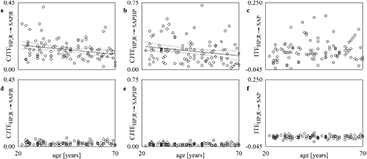
Standard image High-resolution imageFigure 7 shows the simple scatters of the individual values (open circles) of  (figures 7(a) and (d)),
  (figures 7(b) and (e)) and
  (figures 7(c) and (f)) on age at REST. Values were computed over the original data (figures 7(a)–(c)) and surrogates (figures 7(d)–(f)). The linear regression (solid line) and its 95% confidence interval (dotted lines) are plotted when the slope of the regression line is significantly different from 0. When computed over the original data
  (figure 7(a)) and
  (figure 7(b)) were significantly and negatively associated with (r = −0.208, p = 3.77 × 10⁻² and r = −0.241, p = 1.57 × 10⁻² respectively), while
  (figure 7(c)) was unrelated to age (r = −0.106, p = 2.94 × 10⁻¹). When computed over the surrogate data
  (figure 7(d)),
  (figure 7(e)) and
  (figure 7(f)) were steady with age (r = 0.080, p = 4.31 × 10⁻¹, r = 0.055, p = 5.84 × 10⁻¹ and r = −0.011, p = 9.09 × 10⁻¹ respectively).
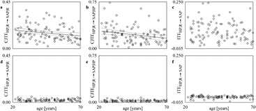
Figure 7. The simple scatters show the individual values (open circles) of  ((a) and (d)),
  ((b) and (e)) and
  ((c) and (f)) on age at REST. The values are computed over the original ((a)–(c)) and surrogate ((d)–(f)) data. When the slope of the regression line is significantly different from 0, the linear regression (solid line) and its 95% confidence interval (dotted lines) are plotted as well. A significant negative correlation of
  and
and  on age is detected only over the original data.
Download figure:
Standard image High-resolution imageFigure 8 has the same structure as figure 7 and shows the same quantities in the same position. At difference with figure 7,  (figures 8(a) and (d)),
  (figures 8(b) and (e)) and
  (figures 8(c) and (f)) were computed during STAND. Conclusions were similar to those at REST. When computed over the original data the correlation coefficients of
  (figure 8(a)),
  (figure 8(b)) and
  (figure 8(c)) on age were −0.268 with p = 7.09 × 10⁻³, −0.223 with p = 2.59 × 10⁻² and 0.123 with p = 2.23 × 10⁻¹ respectively, while, when computed over the surrogates, they were −0.0127 with p = 9.00 × 10⁻¹, −0.0429 with p = 6.72 × 10⁻¹ and −0.0174 with p = 8.64 × 10⁻¹ respectively (figures 8(d)–(f)).
Figure 8. The simple scatters show the individual values (open circles) of  ((a) and (d)),
  ((b) and (e)) and
  ((c) and (f)) on age during STAND. The values are computed over the original ((a)–(c)) and surrogate ((d)–(f)) data. When the slope of the regression line is significantly different from 0, the linear regression (solid line) and its 95% confidence interval (dotted lines) are plotted as well. A significant negative correlation of
  and
and  on age is detected only over the original data.
Download figure:
Standard image High-resolution image
5. Discussion
The main findings of this study can be summarized as follows: (i) at REST redundancy was predominant over synergy in both vascular and cardiac control; (ii) the predominance of redundancy of the cardiac control was not affected by the postural challenge, while STAND reduced the relevance of redundancy of vascular control; (iii) the net redundancy of the cardiac control at REST gradually decreased with age, while that of vascular control remained stable; (iv) during STAND net redundancy of both cardiac and vascular controls was stable with age.
5.1. Significance of the TE in cardiovascular control analysis
We confirm that in healthy subjects indexes assessing the genuine information transferred to HP and SAP variabilities were significantly above the levels set when source signals were artificially uncoupled from the target one (Porta et al 2015b). This conclusion held regardless of the target variable (i.e. HP or SAP), experimental condition (i.e. REST or STAND) and age, thus indicating that the degree of causal coupling from the considered exogenous signals to the target series was always significant. Therefore, we suggest that the absence of a significant causal coupling can be taken as a hallmark of a pathological situation.
5.2. TE in cardiovascular control analysis and postural stressor
When all subjects were pooled together regardless of age we found that STAND decreases the information genuinely transferred from R to HP, while STAND increases the information genuinely transferred from SAP to HP. This finding indicates that the orthostatic challenge reduced the cardiorespiratory coupling (i.e. the HP variability is less influenced by the activity of respiratory centers) as a likely result of vagal inhibition and sympathetic activation in response to the postural stimulus (Montano et al 1994, Cooke et al 1999, Furlan et al 2000, Porta et al 2007, Turianikova et al 2011, Marchi et al 2016a) and increases the cardiac baroreflex coupling (i.e. HP variability is more influenced by SAP changes) as a likely consequence of the increased solicitation of cardiac baroreflex control to react to the central hypovolemia induced by the postural challenge. These conclusions support previous findings obtained with approaches different from that here adopted but computed according to the same paradigm (i.e. the Wiener–Granger causality) (Granger 1980). Indeed, similar conclusions were achieved when the strength of the causal relation from R to HP and from SAP to HP were computed according to a time domain model-based method (Porta et al 2012), a frequency domain technique (Nollo et al 2005) or an information domain model-free method (Nollo et al 2002, Porta et al 2011). Comparable conclusions were drawn using exactly the same approach when central hypovolemia was evoked in a passive way via head-up tilt (Porta et al 2015b, Porta et al 2016a). The information genuinely transferred from HP to SAP was not modified during STAND. Also this result was not surprising given that it is in keeping with the independence of the strength of the coupling from HP to SAP on the tilt table inclination during a graded orthostatic challenge as measured via a model-free Wiener-Granger causality in the information domain (Porta et al 2011). STAND did not affect the information transferred from R to SAP as well. Since the causal relation from HP to SAP describes the contrasting effect of the Frank-Starling law and diastolic runoff on SAP (Baselli et al 1994) and the causal pathway from R to SAP represents the effects of respiratory variations of intrathoracic pressure on SAP via modulation of venous return, stroke volume and cardiac output (Baselli et al 1994, Caiani et al 2000, Elstad and Walloe 2015), their steadiness during STAND suggests that postural change did not modify significantly the relative importance between Frank–Starling law and diastolic runoff and did not impact significantly on the driving action of intrathoracic pressure over venous return, stroke volume and cardiac output.
5.3. TE in cardiovascular control analysis and aging
The information genuinely transferred from SAP to HP along the cardiac baroreflex and from R to HP along the cardiopulmonary pathway was stable with age and this finding held regardless of posture. These results confirm previous conclusions based on a different approach assessing model-based Wiener–Granger causality in the time domain (Porta et al 2014). We conclude that aging modifies the sensitivity of the pathway (e.g. it decreases the cardiac baroreflex sensitivity (Parker Jones et al 2003)) but does not limit the ability of SAP and R to drive HP and to react to a postural stressor. However, we remark that this conclusion might depend on the type of the functional exploited to assess the strength of the causal relation within the same class of method (Porta et al 2016a) and also might vary whether different causality methods are considered. Indeed, some studies detected at REST a decrease of the information transfer from R to HP during senescence when a model-free Wiener–Granger causality approach in the information domain was exploited (Nemati et al 2013, Porta et al 2014). This disagreement might be related to the presence of nonlinear interactions among variables that are disregarded by the present linear approach, while better accounted by model-free approaches. This conjecture deserves a specific study assessing the evolution on nonlinearities with age and linking this evolution with the ability of model-free approach to correctly interpret them. The information genuinely transferred from HP to SAP and from R to SAP progressively decreased with age and this finding held regardless of posture. Also these results confirmed previous findings derived from a time domain model-based Wiener-Granger causality method (Porta et al 2014). These results were interpreted (Porta et al 2014) respectively as an evidence of a reduced importance of the diastolic runoff as a consequence of the increase of the peripheral resistances with age (Laitinen et al 2004) and to the reduced effectiveness of respiratory-related modifications of the intrathoracic pressure in modulating venous return, stroke volume and cardiac output as a likely result of an increased venous pooling and arterial stiffness during senescence (Lakatta and Levy 2003a, 2003b). Remarkably, these results exclude the biasing effect of a relevant confounding factor such as the decrease of respiratory sinus arrhythmia with age (Laitinen et al 2004, Beckers et al 2006) over the information transferred from R to SAP given that HP was conditioned out.
5.4. Significance of the ITE and prevalence of redundancy in cardiovascular control
We originally tested the significance of the ITE in cardiovascular control analysis and we checked the net balance between redundancy and synergy. ITEs from SAP and R to HP and from HP and R to SAP were significantly larger than the corresponding quantities computed after destroying the coupling between the sources and the target, while preserving the dynamics and the distribution of all series. Remarkably, ITE was most frequently positive regardless of the target variable (i.e. HP or SAP) and experimental condition (i.e. REST or STAND), thus indicating a prevalence of redundancy in cardiovascular regulation. We interpret this finding with the necessity of the cardiovascular control to feature a set of commands sharing some common action over the same target. This property of the regulatory system, specifically quantified by the ITE, assures fault tolerance and improves stability of the overall cardiovascular system in the unfortunate situation in which one of the exogenous sources gets impaired or missed. We propose to use the ITE as a highly specific marker to quantity the degree of fault tolerance of the cardiovascular control and stability of the homeostatic regulation.
5.5. ITE in cardiovascular control and postural stressor
We firstly evaluated the effect of a postural stimulus evoking a central hypovolemia on the redundancy of the cardiovascular control. We found that the effect of postural challenge on the redundancy of the cardiovascular control depends on the target variable. Indeed, while the redundant contribution of SAP and R to HP was not significantly modified by STAND, that of HP and R to SAP decreased in response to the postural stimulus. Since redundancy of SAP and R to HP measures the shared information transfer of SAP and R to HP, keeping it high during STAND indicates that baroreflex and cardiopulmonary pathway preserve their shared ability in governing HP. Since their shared ability is likely to be the result of the integration at brainstem level, it might be advisable that this capability is not lost during an important challenge of human being such as STAND. Since redundancy of HP and R to SAP measures the shared information transfer from HP and R to SAP, its decrease during STAND indicates that the mechanical feedforward and the effect of respiratory-related modifications of the intrathoracic pressure lose part of their shared ability in driving SAP. Since this shared ability is more likely to be effective at fast time scales, the decline of respiratory sinus arrhythmia during STAND (Montano et al 1994, Cooke et al 1999, Furlan et al 2000, Porta et al 2007, Turianikova et al 2011, Marchi et al 2016) might play a role in the observed decrement.
5.6. ITE in cardiovascular control and aging
We originally evaluated the evolution of redundancy of the cardiovascular control with age at REST and during STAND. We found that the dependence of the redundancy of the spontaneous variability control on age varies with the target variable (i.e. HP or SAP). Indeed, at REST the shared information transfer from SAP and R to HP gradually decreased with age, while that from HP and R to SAP was steady. Moreover, assigned the target variable (i.e. HP or SAP) the evolution of redundancy depends on the experimental condition. Indeed, the shared information transfer from SAP and R to HP declined with age at REST, while no trend was observed during STAND. We suggest that the progressive decrease of redundancy of cardiac baroreflex and cardiopulmonary pathway to the cardiac control with age indicates an increased frailty of the cardiac control during senescence, a greater likelihood of old people to be exposed to risky situations and a decreased ability to compensate for missing actions of one of the two reflexes. During STAND baroreflex and cardiopulmonary pathway preserve their degree of redundancy with age, thus suggesting a conserved ability to share actions in response to the postural stimulus. Both at REST and during STAND no significant trend of the redundancy of HP and R to SAP was observed. This result could indicate that the shared potentials of the mechanical feedforward and respiratory-related changes of the intrathoracic pressure over SAP was better preserved during aging than that of cardiac baroreflex and cardiopulmonary pathway, thus suggesting a better resilience of vascular control compared to the cardiac one in advanced age.
6. Conclusions
We applied an information domain approach decomposing the JTE from two exogenous sources to a target into the genuine information transfer from each source to the target and a quantity assessing the redundant/synergic contribution of the two causes to the effect to characterize the evolution of the spontaneous cardiovascular variability regulation with age and under a postural stressor. While the relevance of quantifying the genuine information transfer to HP and SAP dynamics with age and under postural stressor was previously proven (Faes et al 2015, Porta et al 2014, 2015a, 2015b, 2016a), the present study stresses the importance of assessing markers of synergy and redundancy. Indeed, this term of the JTE decomposition might be fruitfully exploited to quantify the shared ability of different physiological mechanisms in governing HP and SAP dynamics with promising applications in evaluating the degree of fault tolerance and stability of the cardiovascular control.
Acknowledgments
This study was supported by Fundação de Amparo à Pesquisa do Estado de São Paulo (FAPESP, process number 2010/52070-4) to AMC, by Coordenação de Aperfeiçoamento de Pessoal de Nível Superior (CAPES, process number 23028.007721/2013-4) to AP, ACMT and AMC, and by Conselho Nacional de Desenvolvimento Científico e Tecnológico (CNPq, process number 311938/2013-2) to A.M.C. The funders had no role in study design, data collection and analysis, decision to publish, or preparation of the manuscript.