
Abstract
Objective. Electroencephalograms (EEGs) are often used to monitor brain activity. Several source localization methods have been proposed to estimate the location of brain activity corresponding to EEG readings. However, only a few studies evaluated source localization accuracy from measured EEG using personalized head models in a millimeter resolution. In this study, based on a volume conductor analysis of a high-resolution personalized human head model constructed from magnetic resonance images, a finite difference method was used to solve the forward problem and to reconstruct the field distribution. Approach. We used a personalized segmentation-free head model developed using machine learning techniques, in which the abrupt change of electrical conductivity occurred at the tissue interface is suppressed. Using this model, a smooth field distribution was obtained to address the forward problem. Next, multi-dipole fitting was conducted using EEG measurements for each subject (N = 10 male subjects, age: 22.5 ± 0.5), and the source location and electric field distribution were estimated. Main results. For measured somatosensory evoked potential for electrostimulation to the wrist, a multi-dipole model with lead field matrix computed with the volume conductor model was found to be superior than a single dipole model when using personalized segmentation-free models (6/10). The correlation coefficient between measured and estimated scalp potentials was 0.89 for segmentation-free head models and 0.71 for conventional segmented models. The proposed method is straightforward model development and comparable localization difference of the maximum electric field from the target wrist reported using fMR (i.e. 16.4 ± 5.2 mm) in previous study. For comparison, DUNEuro based on sLORETA was (EEG: 17.0 ± 4.0 mm). In addition, somatosensory evoked magnetic fields obtained by Magnetoencephalography was 25.3 ± 8.5 mm using three-layer sphere and sLORETA. Significance. For measured EEG signals, our procedures using personalized head models demonstrated that effective localization of the somatosensory cortex, which is located in a non-shallower cortex region. This method may be potentially applied for imaging brain activity located in other non-shallow regions.
Export citation and abstract BibTeX RIS

Original content from this work may be used under the terms of the Creative Commons Attribution 4.0 licence. Any further distribution of this work must maintain attribution to the author(s) and the title of the work, journal citation and DOI.
1. Introduction
Somatosensory evoked potentials (SEPs) and magnetic fields (SEFs) have been used for many years to evaluate the disease diagnosis, clinical evaluation, brain function research, and therapeutic effect monitoring recovery from movement disorders (Perot 1973, Fuchs et al 1998). To evoke these potentials, electrical stimulation of peripheral nerve is used, and several components appear in the process of somatosensory pathway reaching the primary somatosensory cortex via the spinal cord, medial lemniscus, and thalamus. Furthermore, it is important to establish a method to accurately estimate the cortical sources because hierarchical processing occurs after the reaching the primary somatosensory cortex (Iwamura 1998).
For brain activity and SEPs and SEFs, minor currents perpendicular to the cortical surface are generated (Mazziotta et al 2001). These currents can be used to monitor the brain activity or responses using electroencephalograms (EEGs), an imaging technique in which the electrical potential on the scalp is measured via a set of attached electrodes (Jurcak et al 2007). However, in EEG imaging, the position of a region that corresponds to specific recorded actions and/or activities must be identified. This technique has various applications for diagnosis, psychology, neuroscience, brain–computer interfaces, and haptics (Acharya et al 2015).
In neuroscientific analyses, as well as in several medical applications, the source of EEG signals or SEPs/SEFs (hereafter called EEG for simplicity) must be localized with a high degree of accuracy (Hallez et al 2007, Acharya et al 2015). Recently, deep learning approaches have been applied for such purposes (Bore et al 2021). The EEG localization accuracy used for the conventional approach may depend on the algorithms used to solve the forward (Hallez et al 2007, Maksymenko et al 2019) and inverse (Friston et al 2008, Acharya et al 2015) problems. In addition to uncertainty and error that originate from the measurements themselves (i.e. due to differences in electrode location and the signal-to-noise ratio) (Cuffin 1998, Wabina and Silpasuwanchai 2022), two key factors influencing localization accuracy—i.e. human head modeling and the forward and inverse problems of the algorithm—are closely related to each other.
Head anatomy was often simplified to homogeneous or multilayer spherical models (Yvert et al 1997, Vorwerk et al 2012, Guttmann-Flury et al 2019). With the development of more sophisticated forms of medical imaging, detailed depictions of anatomical structures (e.g. cerebrospinal fluid (CSF), blood vessels, and skull inhomogeneity) were included in the modeling (Marino et al 1993, Saleheen and Ng 1997, Dannhauer et al 2011, Antonakakis et al 2019, Cuartas Morales et al 2019, Miinalainen et al 2019, Moridera et al 2021, Yavich et al 2021, McCann and Beltrachini 2022). Such models are commonly termed 'volume conductor models.' However, the use of such high-resolution volume conductor models is limited by the computational burden of solving forward problems using conventional approaches. Several effort has been made to reduce demand on computing resources (Laakso and Hirata 2012, Makarov et al 2018).
Several computational electromagnetic methods for analyzing the volume conductor have been used including finite difference, finite element or boundary element methods to solve forward problems. Even using conformal surface modeling (Soldati and Laakso 2020, Conchin et al 2022), this issue inherent to the assignment of tissue-specific conductivity cannot be resolved. Volume conductor modeling and its solution are reciprocal for stimulation and source localization (Dmochowski et al 2017), in addition that the modeling is used for human protection from electromagnetic fields (Reilly and Hirata 2016). One weakness of most volume conductor studies is that computational studies have been conducted using high-resolution finite difference head models, except a few studies (Medani et al 2023).
The assignment of electrical conductivity within biological tissue is another limiting factor when using a volume conductor approach. In general, a single value for electrical conductivity, which is taken from a database, is assigned to all voxels of the corresponding tissue in the segmented model (Reilly and Hirata 2016). The tissue assignment of conductivity could lead to abrupt changes in the tissue conductivity, thereby creating new error for the induced electric field considered by the forward problem (Antonakakis et al 2019, Moridera et al 2021, McCann and Beltrachini 2022). Antonakakis et al (2019) proposed a method of skull modeling in a realistic head model. McCann and Beltrachini (2022) investigated the conductivity of skull inhomogeneity, including aging effect of forward and inverse problems. In addition, the numerical error can be suppressed using a segmentation-free model where tissue conductivity change gradually in space (Moridera et al 2021).
Another factor is the associated algorithm used to solve the inverse problem. A commonly used localization techniques include the lead field matrix (LFM) (Weinstein et al 2000, Fuchs et al 2002, Song et al 2015, Nielsen et al 2018), the minimum norm (MN) method (Hämäläinen and Ilmoniemi 1994, Matsuura and Okabe 1995), beamformer (Jafadideh and Asl 2022), and standard low-resolution brain electromagnetic tomography (sLORETA) (Pascual-Marqui 2002). The LFM is a projection matrix that visualizes the ratio between the electric field of the brain and the electrical potentials at specific electrodes. A large set of variables corresponding to the test dipoles is necessary to construct the LFM. However, the MN method is unsuitable for deep-source localization, since it tends to select a solution with a source close to the surface (Grech et al 2008, Costa et al 2015). In contrast, sLORETA is often used due to its superior accuracy, theoretically, the localization error can be reduced to zero (i.e. statistically insignificant) by standardizing the current density with the covariance matrix of the actual signal. In addition, some studies have reported the sparse signal processing to EEG localization (Liu and Crozier 2004, Xu et al 2007, Yong et al 2008) since here brain activity is localized and sparse. Moreover, several sparse reconstruction methods have been proposed (Wolters et al 2004, Friston et al 2008, Henson et al 2011), including the orthogonal matching pursuit (OMP) algorithm (Pati et al 1993).
In the past, our group computationally demonstrated that high-resolution localization is feasible in segmentation-free head models (Rashed et al 2020a) based using the finite difference method and the OMP algorithm (Moridera et al 2021). This head model was used for intercomparison of induced electric field for field exposure by seven research groups (Diao et al 2023), demonstrating that the computational artifacts have been suppressed and the difference between different research groups was less than 1%. The segmentation-free head models may thus potentially provide greater accuracy than conventional modeling approaches.
The synaptic source activity in the cortical layer is often modeled as a single current dipole source whose position can be estimated by solving an inverse problem (Nunez and Silberstein 2000, Nunez et al 2019). Although multiple dipoles may represent the brain activity best (Ebersole 1994, Rice et al 2013), this approach may not always yield improved localization accuracy due to error, which may originate from multiple error sources as mentioned above.
In this study, we propose a novel process pipeline for multiple-source localization in segmentation-free head models by using the finite difference method and the OMP algorithm. Next, the proposed algorithm was used to assess source localization in non-shallow region using personalized head models and measured EEG signals. To the best of our knowledge, no previous work has successfully demonstrated EEG source localization in such a setup.
The primary novelty of this study is summarized as follows
- (1)A personalized segmentation-free head model developed using subject data leads to improved accuracy of volume conductor development, which helps suppress localized errors associated with the forward and inverse problems common in EEG analysis.
- (2)For measured EEG data, we demonstrated a high level of robustness in the segmentation-free model, and improved the model by applying multi-dipole fitting.
- (3)For a non-shallower source, the accuracy of localization was found to be highly reliable relative to magnetoencephalography (MEG).
The organization of this paper is as follows. Section 2 describes the experimental procedure for EEG signal acquisition due to electrostimulation. Next, we explain the development of an individualized human head model without segmentation from MR images. For individualized head models, the multi-source localization methods used are described. In section 3, we discuss the effectiveness of our proposal by comparing conventional EEG and MEG sources, as well as multi-dipole fitting. Finally, section 4, discusses the results obtained and section 5 summarizes the paper.
2. Materials and methods
2.1. Subjects
Ten healthy volunteers participated in this study (mean age 22.5 ± 0.5 years old). We obtained informed consent from all participants prior to the onset of the experiment, which was approved by the Ethics Committee of the Nagoya Institute of Technology (Approval No. 2020-025). All experiments were performed in accordance with the relevant guidelines and regulations.
2.2. Somatosensory evoked potentials (SEP) and somatosensory evoked magnetic fields (SEF)
First, we conducted electrical stimulation experiments that targeted the primary somatosensory cortex (S1) of the ten healthy subjects. MEG data was obtained using 306 sensors (Elekta Neuromag Vector View, Mind Research Network) in a magnetically shielded room at the National Institute for Physiological Sciences (Japan), and EEG data was obtained using 65 electrodes (QuickAmp 72, Brain Products) at the Nagoya Institute of Technology (Japan). MEG and EEG measurements were obtained on separate days.
SEP and SEF data were obtained by applying electrical stimulation to the median nerve in the subject's right wrist 600 times at 500 ms inter-stimulus intervals. The stimulus intensity of each subject was then increased until the finger responded lightly; thus, all sensory receptive fields were open. EEG electrodes were arranged in accordance with the international 10/10 system (Jurcak et al 2007). In total, we conducted 20 experiments; one for the right and left wrist of each subject.
Experimental data were acquired using a sampling rate of 2 kHz for EEG and 1 kHz for MEG. A bandpass filter (i.e. 3–299.99 Hz) and a notch filter (i.e. 60, 120, 180, and 240 Hz) were applied during signal processing. Next, data were segmented into epochs of 500 ms, and each epoch was averaged after baseline correction using the pre-stimulus interval. In MEG, bad channels were removed by performing frequency analysis on experimental signals and by visually determining power spectral density and time-series signals. For estimation, we also used the somatosensory P20/N20 component, which recorded a tangential dipole located in the Broadman 3b area (Allison et al 1989, Allison et al 1991).
2.3. Source localization using personalized head models
Figure 1 shows the analysis pipeline, which summarizes all steps from data measurement to the source analysis results. First, a realistic human head model for each subject was constructed by applying image processing procedures to MRI data. Second, constructed human head models were used to analyze electric fields and generate the LFM. Next, as described in section 2.1, the acquired EEG signals were processed to obtain N/P20 components from the averaged EEG. Then, inverse problem analysis was performed on the acquired potentials and LFMs to calculate five wave sources and their corresponding weights. Finally, an electric field analysis was performed based on the calculated wave sources to reconstruct the current density distribution, and a weighted average was obtained to estimate the density distribution of currents in the cerebral cortex.
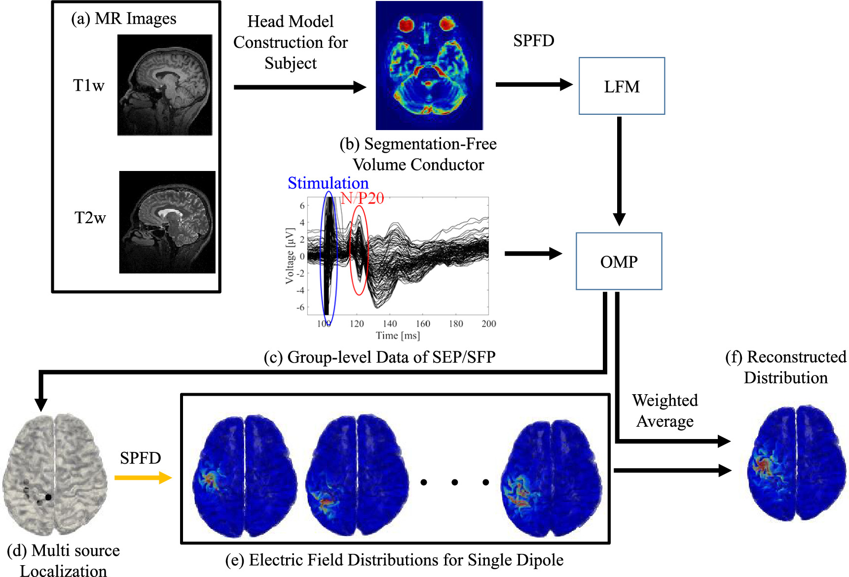
Figure 1. Process pipeline from raw data acquisition to source estimation. First, from (a) T1 and T2 weighted MR images, (b) an individualized head model is developed via machine learning (without segmentation). For each head model, the lead field matrix (LFM) is determined using electromagnetic computation. For EEG signals following electrical stimulation in the subject's right wrist ((c) 600 times with filtering), orthogonal matching pursuit (OMP) is applied for multiple source localization (d). For each distribution of single dipole (e), the distribution is then reconstructed using weighted average (f).
Download figure:
Standard image High-resolution image2.3.1. Head model construction
Schematic explanation of head model development is shown in figure 2. High-resolution T1- and T2-weighted (i.e. T1w and T2w) whole-brain images were acquired at an isotropic resolution of 0.8 mm on a 3.0 T MRI scanner (Magnetom Verio, Siemens Healthneer, Erlangen, Germany). 3D magnetization prepared rapid acquisition with GRE (MPRAGE) sequences were used for T1w images (i.e. TR/TE/TI = 2400/2.24/1060 ms, FA = 8 deg, sagittal slices), while the 3D sampling perfection with application optimized contrast using different FA evolution (SPACE) sequence was used for T2w images (i.e. TR/TE = 3200/560 ms, sagittal slices). The image resolution is improved to 0.5 mm as pre-processing step using three-dimensional nearest neighborhood interpolation algorithm before generating the head models.
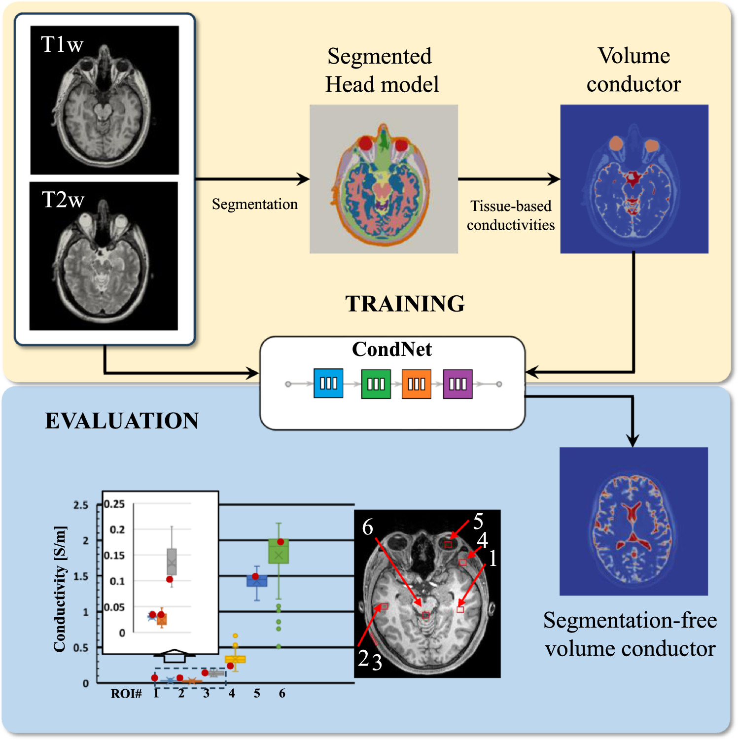
Figure 2. Schematic explanation for the generation of segmentation-free volume conductor model. For induced electric field computation, segmentation-free model is used, and then segmented model is used only as a reference of tissue classification.
Download figure:
Standard image High-resolution imageDifferent approaches are used for improving image quality, such as machine learning and fuzzy techniques (Fischl 2012, Magudeeswaran and Ravichandran 2013, Versaci et al 2015). In this study the dielectric properties of anatomical head models were directly calculated using CondNet, an automatic deep learning estimation model (Rashed et al 2020a). CondNet is a deep learning network that is can directly estimate the dielectric properties from anatomical medical images. The main approach is based on training using T1/T2-weighted MRI and corresponding volume conductors that is generated from standard pipeline (i.e. segmented head models). Then, trained network would be able to automatically generate new volume conductor for new unseen subjects from T1/T2-weighted MRI scans. Technical implementation and network architecture of CondNet is detailed in our earlier work in Rashed et al (2020b) and software is also available as open-source code (https://github.com/erashed/CondNet). CondNet wasD demonstrated to be effective in efficiently estimating dielectric properties such as conductivity and permittivity using a learning-based procedure. Hence, the network assigns non-uniform conductivity values to each image voxel by considering the corresponding T1/T2-weighted MRI scans and water contents. A key feature of volume conductor models generated using CondNet is the smooth transition of conductivity values, particularly at tissue border regions, which effectively reduces artifacts caused by head model generation (i.e. steep differences at tissue boundaries due to the assignment of uniform conductivity values to each tissue) (Rashed et al 2020a). Medical images were acquired at the National Institute of Physiological Science, Japan. The model resolution was 0.5 mm × 0.5 mm × 0.5 mm, which is sufficiently fine that details of the CSF are clearly and efficiently rendered for consideration. Table 1 shows the conductivity value of each tissue as determined using the 4-Cole–Cole model (Gabriel et al 1996). The conductivity of the skin was assumed to be 0.1 S m−1 since the value in the database corresponds to the stratum corneum.
Table 1. Conductivity of each tissue at 10 Hz [40]. Based on these conductivity values, CondNet [39] was applied to develop head models with smooth conductivity transitions.
| Tissue | Conductivity [S m−1] |
|---|---|
| Skin | 0.100 |
| Muscle | 0.202 |
| Fat | 0.038 |
| Bone (cort.) | 0.020 |
| Bone (canc.) | 0.076 |
| Cartilage | 0.161 |
| Gray matter | 0.028 |
| White matter | 0.028 |
| Cerebellum | 0.048 |
| CSF | 2.000 |
| Humor | 1.500 |
| Blood | 0.700 |
| Mucous membrane | 0.0004 |
| Dura | 0.5000 |
2.3.2. Finite difference method
Next, the scalar potential finite difference (SPFD) method (Dawson and Stuchly 1996) was used to compute the scalar potential for each head model. The scalar potential is obtained from Poisson's equation:

Here σ,  and J represent the tissue conductivity, scalar potential, and induced current density, respectively. The potentials of each voxel were defined as unknown. By discretizing equation (1) with a quasi-static approximation, the potential at one node is expressed by using Kirchhoff's current law.

Here n, Sn , ϕn , ω, and q denote the indices of nodes, the edge conductance from the 0th to the nth node (derived from the tissue conductivity of the surrounding voxels), the potential at the nth node, the angular frequency of the wave source, and the electrical charge at the nth node, respectively. The frequency of the wave source was set to 10 Hz, since the alpha band was in the range of 8–13 Hz. The potentials are solved by simultaneous computation of (2) at all nodes.
Using ϕ obtained from (2), the current density is derived as follows:

Here E denotes the electric field induced in the head tissue.
When solving (2), successive over-relaxation (Hadjidimos 2000) was used for the fast iterative convergence of a linear system of equations, which is a variant of the Gauss–Seidel method. As a preconditioner, geometric multi-grid methods were adopted for the calculation (Laakso and Hirata 2012). The number of multi-grid layers was six, and the convergence condition was defined as a relative residual smaller than 10−6.
2.3.3. Calculation of the LFM
The LFM is defined as a projection matrix derived from a current source in discrete gray matter to a potential measured at electrodes placed on the scalp surface (Weinstein et al 2000, Fuchs et al 2002, Song et al 2015). The elements of the LFM represent the ratio of the current density and potential, expressed as follows:

Here L is a M × 3N matrix, and M and N represent the numbers of electrodes and gray matter voxels, respectively. In addition, j is a 3N × 1 vector of the current density strength for each voxel in the x, y, and z directions, while ϕ is an M × 1 potential vector measured by electrodes.
The LFM is commonly constructed using a 'brute force' approach in which forward problem analysis is performed on all voxels that correspond to gray matter in the model (Song et al 2015). However, given the computational cost, calculating the LFM for all voxels in the gray matter is impractical. For our head models with a resolution of 0.5 mm, approximately 3–4 million gray matter voxels (i.e. a total of 30–35 million throughout the head) exist, corresponding to 3 × 3.2 million cases. Instead, the LFM was generated using the reciprocity principle (Weinstein et al 2000, Hallez et al 2007). Here, one electrode is first selected as the ground electrode. After selecting a different electrode (i.e. other than the ground electrode), a current source is assigned to a voxel in the gray matter to compute the electric field via the SPFD method. This procedure is then repeated for the remaining electrodes to construct the following LFM:

Here I is the injection current applied to two electrodes when deriving the LFM.
2.3.4. Inverse problem
Mapping observed scalp potentials to the cerebral cortex in a human head model is the inverse problem of EEG image analysis. As mentioned above, the number of voxels related to gray matter tissues in the human head model is 3–4 million, and a huge amount of computational power would be required to compute all cases. Instead we used the OMP algorithm (Pati et al
1993), with the assumption that all sources are focal and single dipolar (Fuchs et al
1998, Aydin et al
2014, Antonakakis et al
2019). The pseudo code for this algorithm is shown in table 2. The basic principle of the algorithm is to construct sparse vectors by iteratively selecting the most plausible basis vectors from the dictionary matrix. This method can then be used to calculate the sparse current density corresponding to the dictionary matrix. However, the reconstructed  distribution does not follow Kirchhoff's current law. Therefore, we calculated the distribution of current density in the cerebral cortex using the following procedure. First, inverse problem analysis using the OMP algorithm was performed to estimate five coordinates
r
and weights
w
of the estimated sources. Second, at each coordinate
r
of the estimated source location, the current density distribution
j
was analyzed using the SPFD method. Finally, a weighted average based on the weight
w
was used to calculate the current density distribution
distribution does not follow Kirchhoff's current law. Therefore, we calculated the distribution of current density in the cerebral cortex using the following procedure. First, inverse problem analysis using the OMP algorithm was performed to estimate five coordinates
r
and weights
w
of the estimated sources. Second, at each coordinate
r
of the estimated source location, the current density distribution
j
was analyzed using the SPFD method. Finally, a weighted average based on the weight
w
was used to calculate the current density distribution  within the gray matter.
Table 2. Pseudo code for the proposed algorithm based on orthogonal matching pursuit.
Set  as in equation (5) as in equation (5) |
Initialize support vector: 
|
| for loop = 1:5 |
for 
|

|
| end for |
Estimated source location: 
|
Support vector: ![$\hat{{\bf{L}}}={\boldsymbol{[}}\hat{{\bf{L}}}{\boldsymbol{,}}{{\boldsymbol{L}}}_{{\boldsymbol{i}}}{\boldsymbol{]}}$](https://content.cld.iop.org/journals/0031-9155/69/5/055013/revision2/pmbad25c3ieqn9.gif)
|
Reconstruction of current density: 
|
Update residual: 
|
| end for |

2.4. Analysis with sLORETA using brainstorm
Brainstorm (https://neuroimage.usc.edu/brainstorm/Introduction) is an open-source application developed in MATLAB that is specialized for the analysis of brain recordings including MEG, EEG, fNIRS, and ECoG (Tadel et al 2011). In this study, three types of head models were used from Brainstorm three-layer sphere model, boundary Element Models (with OpenMEEG) and the finite element models (with DUNEuro) (Medani et al 2023). Inverse problem analysis was performed by sLORETA, another commonly used software package. With respect to computational memory, the number of candidate source positions was set to 60 000 points on the cortex.
Given that the electrical conductivity of human tissue does not perturb the magnetic field and that tissue permeability is almost identical to that of air, the LFM for MEG was constructed using a sensor-weight overlapping-sphere model (Huang et al 1999). For source estimation, the current density distribution was estimated using MN estimation (Hämäläinen and Ilmoniemi 1994, Grech et al 2008, Asadzadeh et al 2020), and sLORETA (Pascual-Marqui 2002, Song et al 2015) was used for standardization.
3. Results
3.1. Multi-source localization
Figure 3 shows the effect of the number of dipole sources on the residual relative to observed data for the right wrist stimulation of ten subjects. As shown in figure 3(a), the residual for six subjects (6/10) was reduced for multiple dipoles. Moreover, the number of dipoles required was five or less except for two subjects. Next, the estimated potentials for Subject 03 with one or five sources were compared with empirical measurements to consider the effectiveness of multiple fitting. The mean value of the correlation coefficient between the measured and estimated electrical potentials for the 10 subjects was 0.85 (standard deviation (SD): 0.043) for the single dipole (N = 1). Moreover, this improved to 0.87 (SD: 0.040) for N = 5.
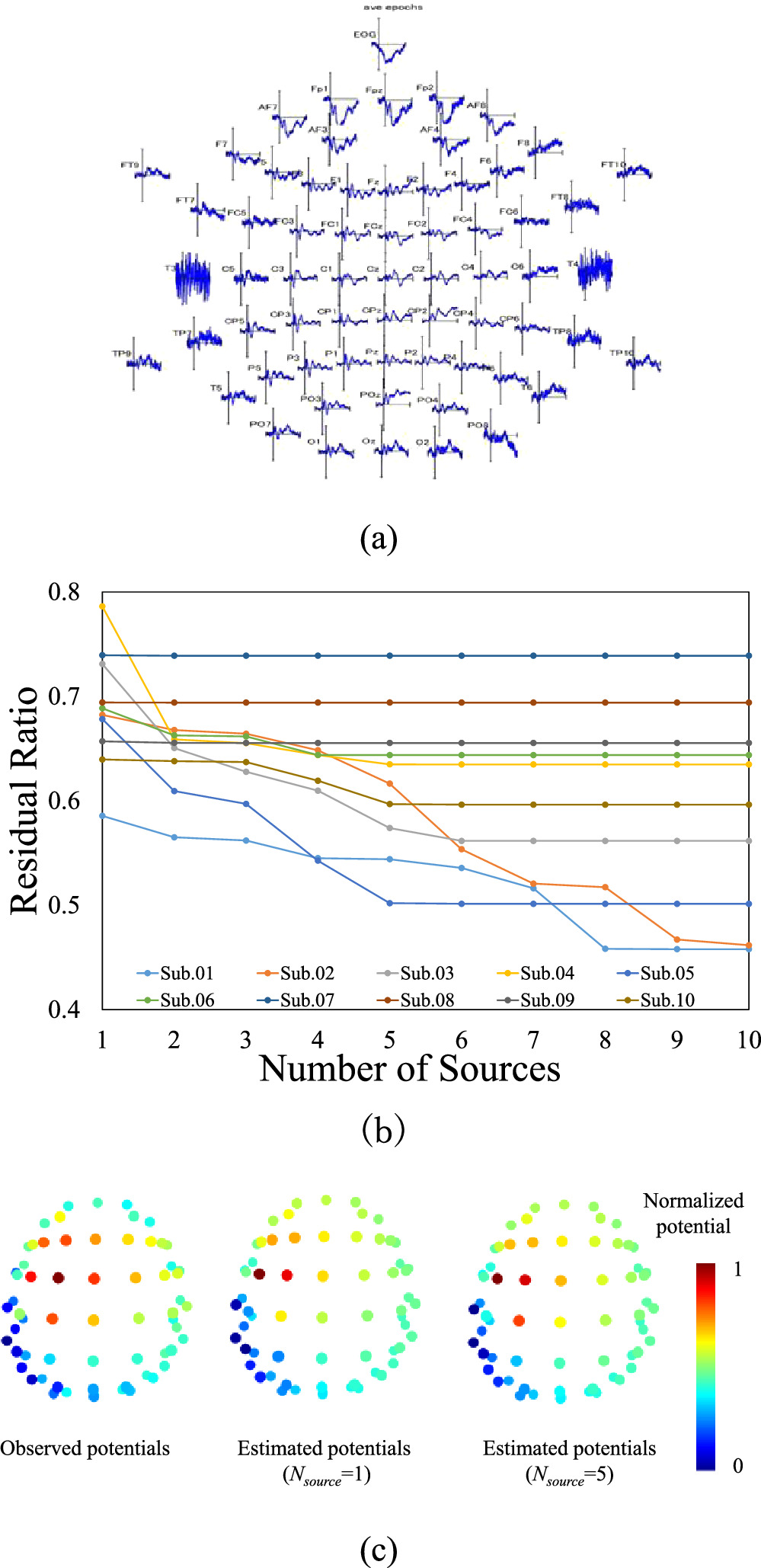
Figure 3. Effect of the number of dipole sources on the residual. (a) An example of preprocessed SEP, (b) residual ratio relative to the observed data for right wrist stimulation of ten subjects. The residual ratio was reduced for multi-source localization (i.e. six subjects). (c) Comparison of observed and estimated potentials (for two values of the number of sources, 1 and 5) for Subject 03. For this subject, the estimated potential of the fifth source localization was closer to the observed one. Normalization was based on the maximum and minimum values of each potential.
Download figure:
Standard image High-resolution image3.2. Localization and their distances
Figure 4 shows the mean coordinates of the areas corresponding to the wrist and finger as estimated by the proposed and different methods in Brainstorm in MNI space. In this test, 20 estimation results were considered in total, i.e. right and left wrist stimulation events for ten subjects. In addition, the reference coordinates estimated by fMRI (Bingel et al 2004, Holmes and Tamè 2019) are also shown. The estimated MNI coordinates and the Euclidean distances from the corresponding reference are listed in table 3. As shown in figure 4, the source location was estimated by all methods to be proximate to the central sulcus.
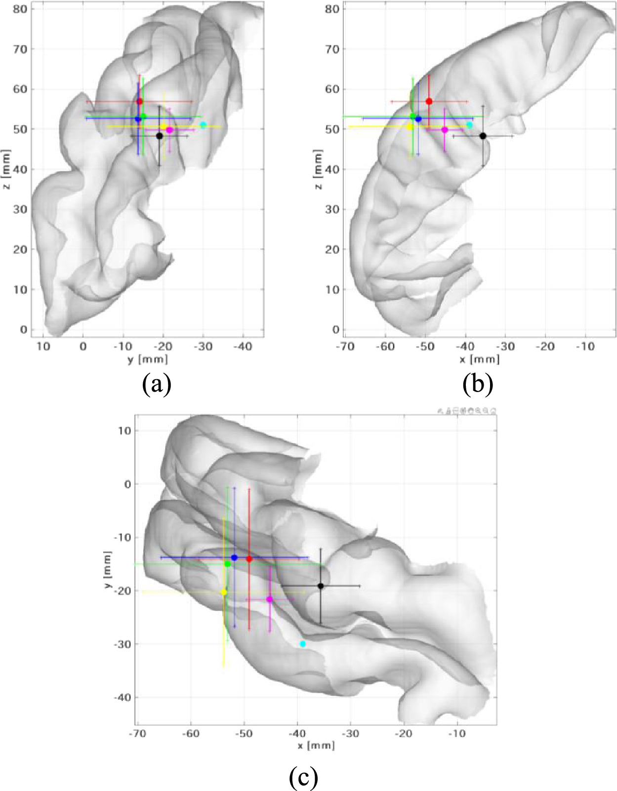
Figure 4. All estimated and reference coordinates for the wrist and finger in MNI space, which represents the (a) sagittal, (b) coronal, and (c) axial slices. Estimated source points are shown for the proposed EEG method (black), EEG with three layer sphere (blue), OpenMEEG (green), DUNEuro (yellow), and conventional MEG (red). Reference source points are also shown for the sites of stimulation in the wrist (cyan) (−39, −30, 51) (Bingel et al 2004) and finger (magenta) (−45.2 ± 4.39, −21.6 ± 6.00, 49.8 ± 5.30) (Holmes and Tamè 2019).
Download figure:
Standard image High-resolution imageTable 3. Estimated and reference coordinates for the wrist and finger in MNI space.
| MNI coordinate [mm] | Euclidean distance [mm] | ||||
|---|---|---|---|---|---|
| x | y | z | Wrist | Finger | |
| Proposed EEG | −35.7 ± 7.3 | −19.1 ± 6.9 | 48.3 ± 7.4 | 16.4 ± 5.2 | 15.1 ± 5.5 |
| Three-layer Sphere | −51.8 ± 13.8 | −13.8 ± 13.0 | 52.6 ± 8.8 | 28.0 ± 10.3 | 21.8 ± 10.0 |
| OpenMEEG | −53.1 ± 15.1 | −15.0 ± 13.8 | 53.1 ± 7.9 | 28.3 ± 10.4 | 22.4 ± 9.8 |
| DUNEuro | −53.9 ± 15.9 | −20.3 ± 13.5 | 50.6 ± 16.2 | 28.4 ± 14.3 | 23.6 ± 14.7 |
| Conventional MEG | −49.1 ± 9.3 | −14.7 ± 13.1 | 56.9 ± 6.5 | 25.3 ± 8.5 | 19.4 ± 8.0 |
As shown in figure 4(b), the locations estimated by the proposed EEG, EEG using three-layer sphere, OpenMEEG, and DUNEuro (sLORETA), and MEG (sLORETA) are indicated by area 3a, area 3b, and area 1, respectively. The estimated coordinate and area of the primary somatosensory cortex are shown in the axial slice (figure 4(c)), the region of the wrist was estimated by the proposed EEG, and the region of the finger was estimated using different method with EEG and MEG.
As shown in table 3, the proposed method had a comparable localization difference (16.4 mm) with the other methods in Brainstorm using EEG (15.6–17.0 mm). Marginally higher localization difference was observed for th feigner location estimated from fMRI in a previous study. The localization with MEG (25.0 mm) was somewhat larger than those obtained using MEG.
3.3. Estimated distribution
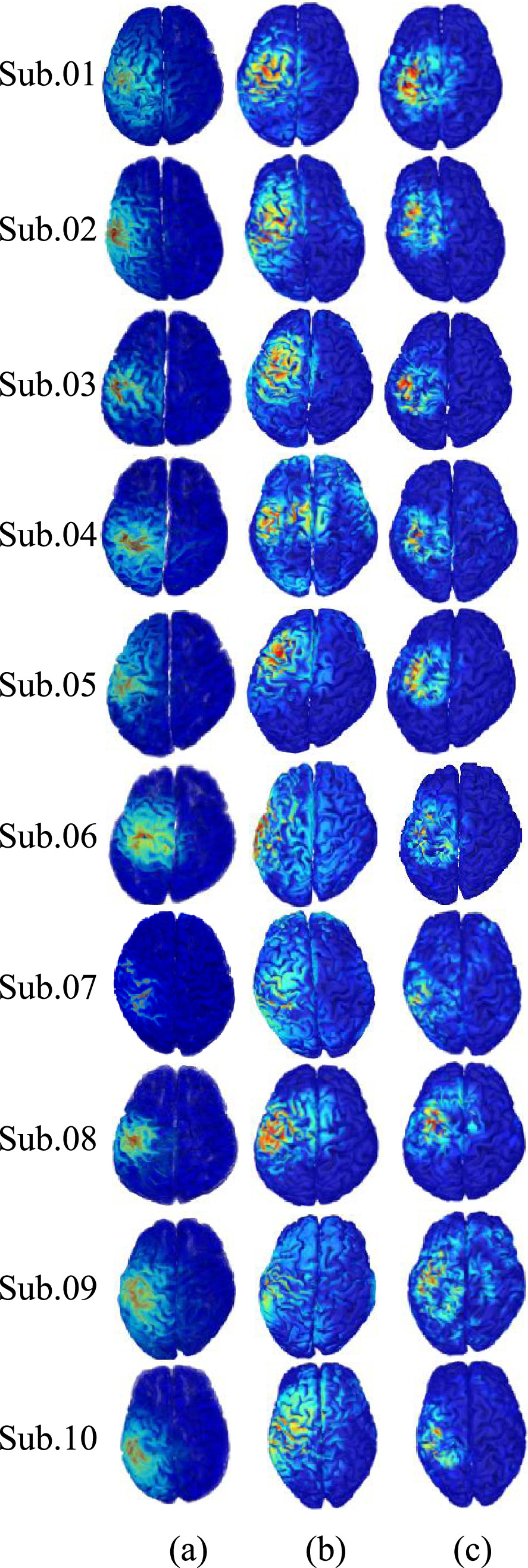
The current density distributions in gray matter obtained for the right wrist stimulation using (a) the proposed method as well as (b) the EEG using three-layer sphere (defined as conventional EEG) and (c) MEG are shown in figure 5. Specifically, figure 5(a) shows that the source location using the proposed method was estimated to be proximate to the central sulcus for all ten subjects. Moreover, as shown in figures 5(b) and (c), the source location determined using the conventional method was estimated to be near the central sulcus for only 80% of subjects. Those subjects showing estimation errors were described as follows: the hot spot shifted anteriorly from the central sulcus in Subjects 02 and 05, and shifted to the left in Subject 06.

Figure 5. Current density distribution on the surface of gray matter obtained using the (a) proposed EEG method, (b) conventional three-layer EEG, and (c) conventional MEG for right wrist stimulation of ten subjects.
Download figure:
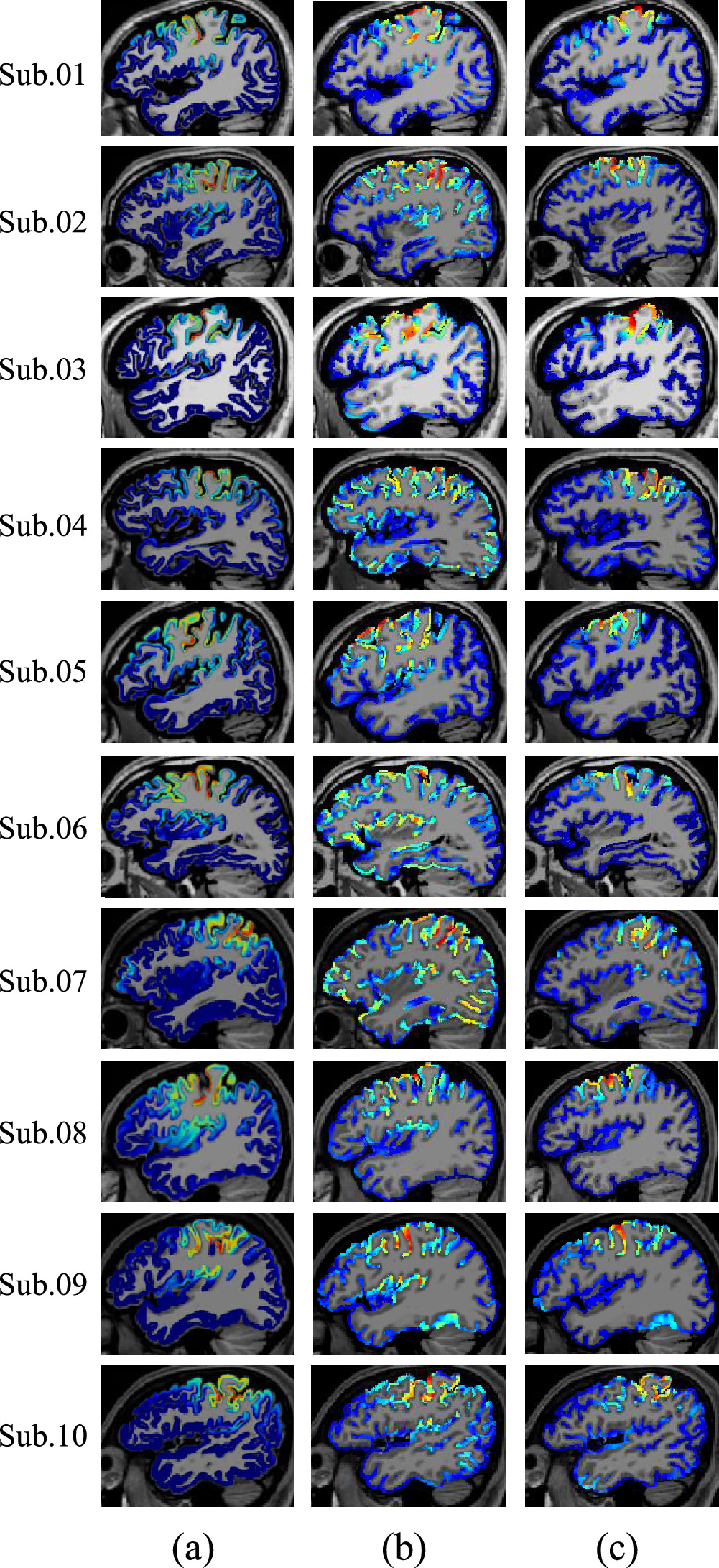
Standard image High-resolution imageTo confirm the detailed current density distribution in the sulci of each subject, the estimated source distribution in sagittal slices is shown in figure 6. The results estimated using the proposed method (figure 6(a)) was distributed throughout three areas: the 3b area, the anterior wall of the postcentral gyrus; the 4 areas, the posterior wall of the precentral gyrus; and the 3a area, the central sulcus. Next, we found that the estimation results of the conventional EEG method (figure 6(b)) were distributed in three regions, namely, the 3a, 3b, and 4 areas; this pattern was the same as that of the proposed method. On the contrary, the estimation results of the conventional method for MEG (figure 6(c)) were distributed in three regions—i.e. the 3b, 1, and 4 areas—and in the apex of the postcentral gyrus. This pattern differed considerably from that of the proposed method. Moreover, no significant difference in estimation accuracy with respect to targeting the 3b and 4 areas or the distribution calculation was observed between the proposed and conventional methods. We only observed such a difference in the tendency of the distribution for the 1 and 3a areas.
Figure 6. Current density distribution on sagittal slices obtained using the (a) proposed EEG method, (b) conventional EEG method, and (c) conventional MEG method for right wrist stimulation of ten subjects.
Download figure:
Standard image High-resolution image
4. Discussion
In this study, we developed high-resolution and segmentation-free personalized human head models for EEG source localization. To generate an accurate LFM, the electric field was computed using a volume conductor model to smooth the gradient of electrical conductivity generated by CondNet [39]. Next, an inverse problem analysis involved applying OMP iteratively for multiple sources using the acquired electrical potential and LFM. Unlike most previous studies, which generally used the finite difference method, here the electric field distribution was reconstructed from the measured electrical potential. As shown in figure 3, the results for six of the ten subjects showed effective multi-dipole fitting. Moreover, for these six subjects, when the number of dipole sources increased from 1 to 5, the average correlation coefficient improved from 0.60 (SD: 0.29) to 0.71 (SD:0.23) using the conventional segmentation model and from 0.87 (SD: 0.043) to 0.89 (SD: 0.04) using the segmentation-free model. This suggests that the segmentation-free model is more robust as well as offering a minor improvement in multi-dipole fitting. A thorough comparison between segmentation and segmentation-free models has been reported previously (Moridera et al 2021).
We then evaluated the source localization of the ten subjects during right and left wrist stimulation using three methods: (a) EEG using the proposed algorithm and (b) EEG methods in Brainstorm, and (c) a MEG method. For the methods in Brainstorm, sLORETA was used to estimate the sources. The localization results of five methods showed marginal differences in predicted location, even in the Brodmann area. The proposed and conventional EEG methods each estimated one of two areas, whereas the conventional MEG method estimated only one area.
In general, methods such as MEG face greater difficulty in recording deep brain activity than EEG methods since the voltage attenuates in proportion to the distance, whereas the magnetic field attenuates in proportion to the square of the distance (Hill et al 2020). This difference was noticeable in our experiment design, in which the stimulus intensity was increased until the subject's fingers responded lightly. Such stimuli may result in a reaction not only in the skin but may also generate proprioceptive information from muscle tissue. In the primary somatosensory cortex, the 3b area is known to be responsible for skin stimuli, whereas the 3a area is for proprioceptive stimuli (Bradley et al 2016). In addition, compared with EEG, MEG also has difficulty in sensing the radial dipole of the sulcus of the brain that corresponds to the 3a area (Valeriani et al 1997). These factors may contribute to the difference in estimated localization between MEG and the EEG methods.
We also note that the difference in the estimated distance in the anterior–posterior direction did not show significant differences between methods. Given that many of the abovementioned factors were common to all methods, differences in estimated location in the anterior–posterior direction may therefore reflect individual differences, such as errors in the transfer from the estimated localization to the standard atlas.
With respect to the estimated localization and the corresponding body part, the proposed method consistently estimated the position close to the wrist, whereas both conventional methods estimated a position close to the finger. The location of the proposed method based on segmentation-free head modeling was most close to that by DUNEuro except in the depth direction. In DUNEuro, the inhomogeneity of skull conductivity was considered (Antonakakis et al 2019), which may be close to the direct estimation of conductivity from MR images in our segmentation-free modeling. One potential difference for this is the multi dipole fitting as the multiple part of the brain was activated for the stimuli. Moreover, two major differences exist between the proposed and conventional methods, namely the head model used to construct the LFM (i.e. anatomical versus spherical models) and the estimation algorithm. In addition, estimation error can also be attributed to the effect of the head model, including differences caused by the head shape and a lack of homogeneity in conductivity. Also, due to the limitation of computational resources using Web-based Brainstorm softwares, the resolution for the localization was limited (60 000); otherwise it is time-consuming (the order of 1 d or more for higher resolution).
Based on the estimated source distribution, the proposed method localized near the central sulcus for all subjects, whereas the conventional method localized with a bias that deviated from the near central sulcus in several subjects (figure 5). Since sLORETA is not known to have a localization bias (Pascual-Marqui 2002, Song et al 2015), this problem can be attributed to the effect of the head model and the localization accuracy in the left and right directions. Figure 6 shows that estimation using the proposed method was distributed in three regions, that is, in the 3a, 3b, and 4 areas, indicating the presence of a source in several regions. Furthermore, the conventional and proposed EEG methods showed the same tendency. In contrast, the MEG method estimated differently, with sources in the 1, 3b, and 4 areas. Thus, no significant difference in estimation accuracy was observed between the proposed and conventional methods when the source was in the 3b or 4 areas.
We also observed differences in the distribution tendency of the 1 and 3a areas among the different estimation methods. If 3a area estimation is feasible, then the fundamental characteristics of the MEG procedure may be a factor contributing to this difference. In general, the MN method has a weakness in judging depth accurately, and can estimate positions closer to the scalp electrode than the true location (Michel and Brunet 2019). However, sLORETA compensates for this weakness by optimizing the localization error by using the data covariance matrix of the EEG signal (Pascual-Marqui 2002). This correction is known to be effective when considering localization errors for a single source, but it is controversial for multiple sources (Hauk et al 2011). For instance, when multiple sources are considered, the estimation of non-shallow sources can be contaminated by leakage from surface sources; i.e. sources with large amplitudes may affect weaker sources. Based on a previous study on cross-talk function, no differences were observed between MN and sLORETA, and noise normalization is not essential (Hauk et al 2011). In contrast, the sparse modeling approach used in the proposed method is not subject to this leakage effect because each estimated source is independent (Hauk et al 2022). Therefore, when multiple sources such as auditory field stimulation are assumed and their amplitudes are considered in isolation, the proposed method using a realistic human head model without segmentation may potentially be more effective than sLORETA.
Table 4 shows a comparison of the solutions to the forward and inverse problems in multiple studies, including the present study (Houzé et al 2011, Klamer et al 2015, Antonakakis et al 2019, Rezaei et al 2021). Other than the present one, only two groups used a personalized head model to solve both the forward (and inverse) problems in a millimeter resolution. We further note that the resolution of the model reported here is finer than that in previous studies, and that we report results for 20 head models, which provides a group-level estimation of source location that was not performed in any previous study.
Table 4. Comparison of forward and inverse problem solutions in this study and in previous studies.
| This study | Houzé et al (2011) | Klamer et al (2015) | Antonakakis et al (2019) | Rezaei et al (2021) | |
|---|---|---|---|---|---|
| Localization method | OMP | BESA | LORETA | single dipole scans | RAMUS |
| Forward problem resolution | 0.5 × 0.5 × 0.5 mm | — | — | 1 mm FE mesh | 1 mm FE mesh |
| Solution space | 0.5 × 0.5 × 0.5 mm | 4 × 4 × 4 mm | — | 1 mm FE mesh | 1 mm FE mesh |
| Number of electrodes | 64 | 128 | 256 | 80 | 74 |
| Number of models | 10(20) | 10 | 14 | 5 | 3 |
| Personalized head | Yes | No | No | Yes | Yes |
This study also has notable limitations. First, the number of subjects was limited to 20 hemispheres, i.e. two each from 10 subjects. This small sample size may have marginally affected the difference of estimated location (see table 3); we observed an improvement of 1–2 mm when considering the other hemisphere (i.e. opposite wrist stimulation). For healthy subjects subjected to electrostimulation, the electric field distribution was stable for subjects 5–10 (Laakso et al 2016), and electrostimulation and the EEG electric field are reciprocal (Dmochowski et al 2017).
We have demonstrated our proposal with the processing of somatosensory information. However, considering a common neural mechanism in the visual and auditory information processing and motor cortex, our proposal would be broadly applicable for analysis of EEG signal.
5. Conclusion
In this study, we propose a novel pipeline for the localization of multi-dipole sources using a personalized head model reconstructed from subject image data. For this model, the tissue electrical conductivity is pre-assigned but changed gradually based on MR images. During electrical stimulation of the median nerve, multi-dipole source localization was more effective in six subjects of healthy adults (6/10) than localization using a single dipole. Furthermore, we found that the proposed method had a smaller difference of the localization with respect to the position of the maximum electric field from the target wrist compared to conventional approaches based on sLORETA. Future research should further evaluate the proposed algorithm for localization of other non-shallow sources, as well as test its potential use for medical applications such as seizure monitoring (Claassen et al 2004) and the diagnosis of diseases (Dauwels et al 2010).
Acknowledgments
This study was supported by JSPS KAKENHI 21H04956.
Data availability statement
The data cannot be made publicly available upon publication because they contain sensitive personal information. The data that support the findings of this study are available upon reasonable request from the authors.