
Abstract
Objective. Gradient-based optimization using algorithmic derivatives can be a useful technique to improve engineering designs with respect to a computer-implemented objective function. Likewise, uncertainty quantification through computer simulations can be carried out by means of derivatives of the computer simulation. However, the effectiveness of these techniques depends on how 'well-linearizable' the software is. In this study, we assess how promising derivative information of a typical proton computed tomography (pCT) scan computer simulation is for the aforementioned applications. Approach. This study is mainly based on numerical experiments, in which we repeatedly evaluate three representative computational steps with perturbed input values. We support our observations with a review of the algorithmic steps and arithmetic operations performed by the software, using debugging techniques. Main results. The model-based iterative reconstruction (MBIR) subprocedure (at the end of the software pipeline) and the Monte Carlo (MC) simulation (at the beginning) were piecewise differentiable. However, the observed high density and magnitude of jumps was likely to preclude most meaningful uses of the derivatives. Jumps in the MBIR function arose from the discrete computation of the set of voxels intersected by a proton path, and could be reduced in magnitude by a 'fuzzy voxels' approach. The investigated jumps in the MC function arose from local changes in the control flow that affected the amount of consumed random numbers. The tracking algorithm solves an inherently non-differentiable problem. Significance. Besides the technical challenges of merely applying AD to existing software projects, the MC and MBIR codes must be adapted to compute smoother functions. For the MBIR code, we presented one possible approach for this while for the MC code, this will be subject to further research. For the tracking subprocedure, further research on surrogate models is necessary.
Export citation and abstract BibTeX RIS

Original content from this work may be used under the terms of the Creative Commons Attribution 4.0 licence. Any further distribution of this work must maintain attribution to the author(s) and the title of the work, journal citation and DOI.
1. Introduction
The option of treating cancer using beams of high-energy charged particles (mainly protons) is becoming more and more available on a world-wide scale. The main advantage over conventional x-ray radiotherapy lies in a possibly lower dose deposited outside the tumor, as the energy deposition of protons is concentrated around the so-called Bragg peak. The depth of the Bragg peak depends on the beam energy and the relative stopping power (RSP) of the tissue it traverses. Thus, treatment planning relies on a three-dimensional RSP image of the patient. In the state of the art calibration procedure of x-ray CT for proton therapy, scanner-specific look-up tables are used to convert the information retrieved from x-ray (single-energy or dual-energy) CT acquisitions into an RSP image: this approach comes with an uncertainty of the Bragg peak location of up to 3% of the range (Paganetti 2012, Yang et al 2012, Wohlfahrt and Richter 2020). On the other hand, the direct reconstruction of a proton CT image using a high-energy proton beam and a particle detector has been shown to be intrinsically more accurate (Yang et al 2010, Dedes et al 2019).
To this end, the Bergen proton computed tomography (pCT) collaboration (Alme et al 2020) is designing and building a high-granularity digital tracking calorimeter (DTC) as a clinical prototype to be used as proton imaging device in existing treatment facilities for proton therapy. Its sensitive hardware consists of two tracking and 41 calorimeter layers of 108 ALPIDE (ALICE pixel detector) chips (Aglieri Rinella 2017) each. After traversing the patient, energetic protons will activate pixel clusters around their tracks in each layer until they are stopped, as shown in figure 1. In each read-out cycle, the layer-wise binary activation images from hundreds of protons are collected and used to reconstruct the protons' paths and ranges through the detector and thus their residual direction and energy after leaving the patient. Based on this data from various beam positions and directions, a model-based iterative reconstruction (MBIR) algorithm reconstructs the three-dimensional RSP image of the patient. The reconstructions of proton histories and of the RSP image are displayed as two main subprocedures in figure 2(a), along with a Monte Carlo simulation subprocedure to generate the detector output instead of a real device for testing and optimization purposes.
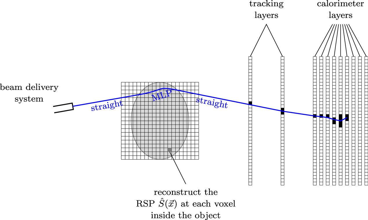
Figure 1. Schematic figure of the scanning process.
Download figure:
Standard image High-resolution image
Figure 2. Computational steps in the pCT reconstruction pipeline. (a) Overview of the pCT reconstruction pipeline. (b) Computational steps of the Monte Carlo Simulation. (c) Computational steps of the proton reconstruction subprocedure. (d) Computational steps of the MBIR subprocedure.
Download figure:
Standard image High-resolution imageAlgorithmic differentiation (AD) (Griewank and Walther 2008, Naumann 2011) is a set of techniques to efficiently obtain precise derivatives of a mathematical function given by a computer program. Such derivatives have been successfully used to solve optimization problems in various contexts, such as machine learning (ML) (Baydin et al 2017) and computational fluid dynamics (CFD) (Albring et al 2016), and AD is currently also adopted in the fundamental physics community for detector optimization (Baydin et al 2021, Strong et al 2022a, 2022b, Dorigo et al 2023). In all of these applications, an objective or loss function is formulated, which maps
- a set of n inputs for a design choice: e.g. weights of a neural network in ML, an airfoil shape in CFD, or, prospectively, geometry and material composition parameters of a detector; to
- a single scalar output representing how well this design performs: e.g. the training error in ML, aerodynamic drag or lift in CFD, or application-specific measures of physics performance of a detector.
Derivatives of the objective function with respect to its inputs are obtained via reverse-mode AD. A gradient-based optimization algorithm uses these derivatives to find sets of input values that minimize (or maximize) the objective function. This way it trains the ML model, finds an optimal aerodynamic design choice, or—which is what this work prepares the way for—finds optimal detector designs.
The advantage of gradient-based optimization with reverse-mode algorithmic derivatives, compared with gradient-free optimization algorithms like manual tuning of individual parameters (in the easiest case), is that a higher number of design parameters can be jointly optimized, the mathematical theory e.g. on convergence speeds is further developed, and optimality criteria based on the gradient give a less arbitrary criterion on when to stop searching for even better designs. Aside from optimization, particular methodologies for uncertainty quantification (UQ) involve derivatives.
Integrating AD into a bundle of big and complex pieces of software is usually a major technical effort. In addition to that, (algorithmic) derivatives are most useful for gradient-based optimization and UQ if the differentiated function is sufficiently smooth. Non-differentiable operations such as rounding employed to find the voxel that contains a given point, floating-point comparisons to determine the physics process happening next, and stochasticity of a Monte-Carlo simulation in general, may reduce the value of derivative information depending on how often they appear. We thus cannot expect the ultimate goal of our research line, an fully differentiated pipeline allowing for an efficient minimization of the average error of the reconstructed RSP image, to work out-of-the-box after AD has been integrated in all parts of the pCT pipeline. In this work, we study how smooth three representative substeps of the pCT reconstruction process are. To this end, we observe reactions of specific outputs on changes in a single input parameter keeping the other inputs fixed, explain our observations, and propose mitigation measures for observed non-smooth behaviour.
In section 2.1, we summarize all the computational steps of the software pipeline in greater detail. Section 2.2 is a general introduction into the purpose and calculation of derivatives of computer programs. The numerical experiments are outlined in section 2.3 and their results are stated in section 3. In section 4, we analyze the observed discontinuous or non-differentiable behaviour and propose ways to mitigate it, and close with a summary and conclusions in section 5.
2. Methods
2.1. Simulation of proton CT data acquisition and processing
2.1.1. Foundations
When energetic protons pass through matter, they slow down in a stochastic way, mainly due to inelastic interactions with the bound electrons. The average rate  of kinetic energy E lost per travelled length s is called stopping power. We denote it by
  , indicating its dependency on the current energy E of the proton and the local material present at location
  . Using the symbol Sw
(E) for the stopping power of water at the energy E, the RSP is defined as
. Using the symbol Sw
(E) for the stopping power of water at the energy E, the RSP is defined as

The dependency on E has been dropped in the notation because in the relevant range between 30 and 200 MeV, the RSP is essentially energy independent (Hurley et al 2012).
Separating variables and integrating, one obtains

This integral value is called the water-equivalent path length (WEPL).
In list-mode, or single-event, pCT imaging, millions of protons are sent through the patient, and their positions, directions and energies are recorded separately, both before entering and after leaving the patient. In the setup conceived by the Bergen pCT collaboration and sketched in figure 1, the exit measurements are performed by the tracking layers of the DTC, through the processing steps outlined in section 2.1.3. The setup at hand infers the positions and directions of entering protons from the beam delivery monitoring system, and therefore does not require a second pair of tracking layers in front of the patient; this has been shown sufficiently accurate for dose-planning purposes through MC simulation studies (Sølie et al 2020). For other pCT (and proton radiography) projects, see e.g. Pemler et al (1999), Hurley et al (2012), Scaringella et al (2013), Saraya et al (2014), Naimuddin et al (2016), Esposito et al (2018), Mattiazzo et al (2018), Meyer et al (2020), DeJongh et al (2021).
2.1.2. Monte Carlo subprocedure
Figure 2(b) displays the intermediate variables and computational steps of the Monte Carlo subprocedure to simulate the detector. Its central step is the open-source software GATE (Jan et al 2004) for simulations in medical imaging and radiotherapy, based on the Geant4 toolkit (Agostinelli et al 2003, Allison et al 2006, 2016). Given a description of the relevant properties of the detector-patient setup like detector geometry and physics parameters and the original RSP distribution inside the patient, GATE produces stochastically independent paths of single particles through the setup. Whenever interactions occur, with a certain probability distribution, the turnout for the proton at hand is decided by a random number from a pseudo-random number generator (RNG). Such random numbers represent 'true' randomness sufficiently well (as measured by specific statistical tests) but are computed deterministically from an initial state called the seed.
The epitaxial layers of the ALPIDE chips are modelled as single crystalSD volumes in GATE, so the positions and energy losses of all charged particles passing these volumes are recorded. Additional code converts these hits to clusters of pixels activated by electron diffusion around the track, whose size corresponds to the recorded energy loss (Pettersen et al 2019, Tambave et al 2020). Depending on the exact choice of parameters, about 100 protons pass through the DTC during one read-out cycle of the real detector.
2.1.3. Proton track reconstruction
Figure 2(c) displays the computational steps to convert the binary activation images per layer and read-out cycle, either produced by the real detector or by the Monte Carlo procedure in section 2.1.2, back to continuous coordinates and energies of protons.
Orthogonally neighbouring activated pixels are grouped into clusters per layer and read-out cycle, as they likely originate from one proton. The proton's coordinate is given by the cluster's center of mass and its energy deposition is related to the size of the cluster (Pettersen et al 2017, Tambave et al 2020).
In the tracking step, a track-following procedure (Strandlie and Frühwirth 2010) attempts to match clusters in bordering layers likely belonging to the same particle trajectory. The angular change between the extrapolation of a growing track and cluster candidates in a given layer is minimized in a recursive fashion (Pettersen et al 2019, 2020).
Based on the cluster coordinates in the two tracking layers of the DTC, the position and direction of the proton exiting the patient can be inferred. A vector x(PD) stores this data together with the position and direction of the beam source.
The proton's residual WEPL before entering the detector can be estimated by a fit of the Bragg-Kleeman equation of Bortfeld (Bortfeld 1997, Pettersen et al 2018) to the energy depositions per layer (Pettersen et al 2019). Its difference to the initial beam's WEPL is stored in x(W). Failures of the tracking algorithms are usually due to pair-wise confusion between tracks from multiple Coulomb scattering (MCS), to the merging of close clusters, or to high-angle scattering. To this end, tracks with an unexpected distribution of energy depositions are attributed to secondary particles or mismatches in the tracking algorithm, and filtered out (Pettersen et al 2021).
2.1.4. MBIR subprocedure
Model-based iterative reconstruction algorithms repeatedly update the RSP image to make it a better and better fit to the measurements of x(PD), x(W), according to the model equations (2).
The paths of the protons in the air gaps between the beam delivery system, the patient and the DTC can be assumed to be straight rays. Inside the patient, they are stochastic and unknown due to electromagnetic (MCS) and nuclear interactions with atomic nuclei. Using the model of MCS by Lynch and Dahl (1991) and Gottschalk et al (1993), and given projections of the positions and directions x(PD) from section 2.1.3 to the hull of the scanned object, the most likely path (MLP) can be analytically approximated in a maximum likelihood formalism (Schulte et al 2008). The extended MLP formalism (Krah et al 2018) also takes uncertainties of the positions and directions into account: this is especially important when the front tracker is omitted, since the beam distribution is modeled using this formalism. Alternatively, a weighted cubic spline is a good approximation of the MLP (Collins-Fekete et al 2017). The WEPL of the proton is the integral of the RSP along the estimated path, and has also been reconstructed (as described in section 2.1.3) as x(W). This leads to a linear system of equations for the list y of all voxels of the RSP image,

The entry (i,j) of the matrix  stores how much the RSP at voxel j influences the WEPL of proton i; this value is related to the length of intersection of the proton's path and the voxel's volume, and thus depends on x(PD). As each proton passes through a minor fraction of all voxel volumes, A is typically sparse. Instead of the approximate length of intersection, a constant chordlength, mean chord length or effective mean chord length (Penfold et al
2009) can be used to determine the matrix elements. As an alternative, we also study a 'thick paths' or 'fuzzy voxels' approach where points on the path are assumed to influence a wider stencil of surrounding voxels, with a weight that decreases with distance.
stores how much the RSP at voxel j influences the WEPL of proton i; this value is related to the length of intersection of the proton's path and the voxel's volume, and thus depends on x(PD). As each proton passes through a minor fraction of all voxel volumes, A is typically sparse. Instead of the approximate length of intersection, a constant chordlength, mean chord length or effective mean chord length (Penfold et al
2009) can be used to determine the matrix elements. As an alternative, we also study a 'thick paths' or 'fuzzy voxels' approach where points on the path are assumed to influence a wider stencil of surrounding voxels, with a weight that decreases with distance.
The matrix A is not a square matrix as the number of protons is independent of the dimensions of the RSP image. Therefore 'solving (3)' is either meant in the least-squares sense, or additional objectives like noise reduction are taken into account via regularization or superiorization (Penfold et al 2010).
For simplicity, this study is not concerned with algorithms to determine the hull of the scanned object. Assuming that the hull is known, the two main computational steps of the MBIR subprocedure, generating the matrix  and solving the system (3), are displayed in figure 2(b). Several implementations of x-ray MBIR algorithms (van Aarle et al
2015, Biguri et al
2016) actually do not store the matrix in memory explicitly, because even in a sparse format it would be to large (Biguri et al
2016). Rather, they implement matrix-free solvers like ART, SIRT, SART, DROP (diagonally relaxed orthogonal projections) (Penfold and Censor 2015) or LSCG (least squares conjugate gradient). These access the matrix only in specific ways, e.g. via (possibly transposed) matrix-vector products or calculating norms of all rows. The matrix elements can thus be regenerated on-the-fly to perform the specific operation demanded by the solver. In pCT, it is best to structure these operations as policies to be applied for each row of A: Due to the bent paths of protons, it is more efficient to make steps along a path and detect all the voxels it meets, rather than the other way round. Parallel architectures like GPUs can provide a significant speedup for operations whose policies can be executed concurrently for many rows.
and solving the system (3), are displayed in figure 2(b). Several implementations of x-ray MBIR algorithms (van Aarle et al
2015, Biguri et al
2016) actually do not store the matrix in memory explicitly, because even in a sparse format it would be to large (Biguri et al
2016). Rather, they implement matrix-free solvers like ART, SIRT, SART, DROP (diagonally relaxed orthogonal projections) (Penfold and Censor 2015) or LSCG (least squares conjugate gradient). These access the matrix only in specific ways, e.g. via (possibly transposed) matrix-vector products or calculating norms of all rows. The matrix elements can thus be regenerated on-the-fly to perform the specific operation demanded by the solver. In pCT, it is best to structure these operations as policies to be applied for each row of A: Due to the bent paths of protons, it is more efficient to make steps along a path and detect all the voxels it meets, rather than the other way round. Parallel architectures like GPUs can provide a significant speedup for operations whose policies can be executed concurrently for many rows.
2.2. Derivatives of algorithms
2.2.1. Differentiability
Any computer program that computes a vector  of output variables based on a vector
  of input variables defines a function
  , that maps x to y. Typically, f is differentiable for almost all x, because we may think of a computer program as a big composition of elementary functions like +, ·,
  ,
,  , ∣ · ∣, and apply the chain rule. Possible reasons why f could not be differentiable at a particular x include the following:
- An elementary function is evaluated at an argument where it is not differentiable, like the abs function ∣ · ∣ at 0.
- An elementary function is evaluated at an argument where it is not even continuous, like rounding at
 for integers k.
 - An elementary function is evaluated at an argument where it is not even defined, like division by zero.
- A control flow primitive such as if or while makes a comparison like a = b, a > b, a < b, a ≥ b or a ≤ b between two expressions a, b that actually have the same value for the particular input x.

A computer-implemented function f is likely to be non-differentiable (almost) everywhere if it operates directly on digital floating-point representations of real numbers with, e.g., bitshifts or bitwise logical operations. This comprises cryptographic and data-compression algorithms, as well as RNG primitives like taking a sample from a uniform distribution between 0 and 1.
2.2.2. Taylor's theorem
Although differentiability and derivatives are local concepts, they can be used for extrapolation by Taylor's theorem. A precise statement (Anderson 2021) in first order is that if f is twice continuously differentiable, for each  there are constants
  such that the error of the linearization

is bounded by  for all x with
  . The constant C depends on how steep
  is. Even if the differentiability requirements are violated, the Taylor expansion (4) is frequently used for the applications discussed in the next sections 2.2.3 and 2.2.4. Heuristically, the higher the 'amount' or 'density' of the non-differentiable points x listed above is, the less well these applications perform. To assess the range in which the linearization (4) is valid, one can plot
  against
  and compare to the graph of a proportionality relation. We call it the linearizability range.
2.2.3. Quantification of uncertainty
If the value of an input x is approximated by  and the resulting uncertainty of f(x) is sought,
  contains the relevant information to measure the amplification of errors: according to the Taylor expansion (4), the deviation of x from
  gives rise to an approximate deviation of f(x) from
  by
by  .
.
For small local perturbations, a more specific analysis is possible when we model the uncertainty in the input x using a Gaussian distribution with mean  and covariance matrix Σx
, and replace f with its linear approximation (4). For a linear function f, the output f(x) is a Gaussian distribution with mean
and covariance matrix Σx
, and replace f with its linear approximation (4). For a linear function f, the output f(x) is a Gaussian distribution with mean  and covariance matrix

We are interested in uncertainties of the reconstructed RSP image as a result of the MBIR subprocedure, or the uncertainties of results of further image processing like contour lines (Aehle and Leonhardt 2021). Possible input variables of known uncertainty are the detector output or reconstructed proton paths. All steps in the pipeline from this input to the output must be differentiated in order to apply (5). Since the above input variables are defined after the Monte Carlo subprocedure (see figure 2(a)), the differentiation of this step is not required.
Uncertainties in the input should be 'unlikely' to go beyond the linearizability range. Otherwise, f is not approximated well by its linearization for a significant amount of possible inputs x and (5) cannot be used, as illustrated in figure 3.

Figure 3. A function f, shown by the dash-dotted plot in the central box, is applied to a Gaussian random variable x whose probability density function (PDF) is shown in the bottom graph. The orange graph in the left box conveys the true distribution of f(x), whereas the normal distribution with variance according to (5) is shown in blue. Cited from Aehle and Leonhardt (2021). (a) Good approximation, because f is approximatively linear in e.g. a σ-envelope around  . (b) Bad approximation, because much of the input distribution extends beyond the linearizability range around
  . Reproduced with permission from Aehle and Leonhardt (2021).
Download figure:
Standard image High-resolution imageNo matter how non-smooth f is, Monte Carlo simulation can be used alternatively to propagate a random variable x through a computer program f and estimate the statistical properties of the random variable f(x). The more samples are used, the better the Monte Carlo estimate becomes, but the more run-time must be spent.
2.2.4. Gradient-based optimization
In the case that f has a single output variable (m = 1), optimization seeks to find a value for x that minimizes (or maximizes) this objective function. Gradient-based optimization methods have already been employed for CT reconstruction, with the voxel values of the CT image as input variables and the distance between the resulting and the actual measurements as an objective function that ought to be minimized (Sidky et al 2012); image quality measures can also be part of the objective function (Choi et al 2010).
In contrast, our work heads towards the long-time goal of finding optimal parameters of a pCT setup, including geometric parameters, material compositions, and algorithmic parameters of the reconstruction software. In this context, a meaningful objective function is given by the error of the reconstructed RSP image compared with the original RSP used in the Monte-Carlo simulation (Dorigo et al 2023), averaged over a collection of such original RSP images.
The idea behind gradient-based optimization is that as the gradient points into the direction of steepest ascent according to (4), shifting x in the opposite direction should make f(x) smaller. Many training algorithms in machine learning (ML) also belong to this category, with the training error of the ML model as the objective function. If f is differentiable and its linearizability range is sufficiently large, gradient-based optimization algorithms can find minima after a reasonable number of descent steps.
For the long-term goal described above, in general, all parts of the objective function (like the pipeline in figure 2(a)) would have to be differentiated, including the Monte Carlo simulation. Strong et al (2022a, 2022b) have demonstrated gradient-based optimization for a muon tomography setup (e.g. determining the optimal positions of muon tracker planes), avoiding to differentiate Monte Carlo codes by neglecting the effect of the setup on the particle trajectories.
As an alternative to gradient-based optimization algorithms, many gradient-free optimization methods have been proposed to avoid evaluating the gradient of f (Larson et al 2019). The most basic instance of such an algorithm would be to select a finite set of configurations x (e.g. on a grid or by random), evaluate f on all of them, and pick the minimizer within this set. Simulated annealing explores the configuration space by making steps in random directions. Surrogate models can be trained to predict f (or its gradient), and then be used for optimization.
In many application domains such as computational fluid dynamics (Albring et al 2016) and ML training (Baydin et al 2017), gradient-based optimization methods are however preferred for several reasons. They provide criteria to decide whether an actual minimum has been reached (e.g. when the gradient becomes small), and for specific classes of functions, mathematical statements guarantee convergence to mimima with certain convergence speeds (Nesterov 2018). But mainly, they perform well even if the number of design parameters is high. Only few gradient-free optimization algorithms are able to deal with n ≥ 300 parameters (Rios and Sahinidis 2013), whereas gradient-based optimization based on backpropagation can train ML models with billions of parameters (Brown et al 2020).
2.2.5. Algorithmic differentiation
The classical ways to obtain derivatives of a computer-implemented function f, required for the applications described in sections 2.2.3 and 2.2.4, are analytical (using differentiation rules, possible only for simple programs) or numerical (using difference quotients, inexact). Ideally, algorithmic differentiation combines their respective advantages being exact and easy applicable; moreover, the reverse mode of AD provides the gradient of an objective function f in a run-time proportional to the run-time of f, independently of the number of design parameters (Griewank and Walther 2008).
AD tools facilitate the application of AD to an existing codebase; specifically, operator overloading type AD tools intercept floating-point arithmetic operators and math functions, and insert AD logic that keeps track of derivatives with respect to input variables (in the forward mode), or records an arithmetic evaluation tree (in the reverse mode). As examples for such tools, we may cite ADOL-C (Walther and Griewank 2012), CoDiPack (Sagebaum et al 2019), the autograd tool (Maclaurin et al 2015) used by PyTorch (Paszke et al 2019), and the internal AD tool of TensorFlow (Abadi et al 2016). The machine-code based tool Derivgrind (Aehle et al 2022a, 2022b) may offer a chance to integrate AD into cross-language and partially closed-source software projects. For an overview of tools and applications, visit https://autodiff.org.
While these tools can often be applied 'blindly' to any computer program to obtain algorithmic derivatives in an 'automatic' fashion, further program-specific adaptations might be necessary. For example, the new datatype of an operator overloading tool might break assumptions on the size or format of the floating-point type that were hard-coded in the original program. Concerning complex simulations, techniques like checkpointing (Dauvergne and Hascoët 2006, Naumann and Toit 2018) or reverse accumulation can reduce the memory consumption of the tape in reverse mode but require manual modifications of the primal program.
Another major reason for revisiting the primal code is given by the fact that it is usually only an approximation of the real-world process. Good function approximation does not guarantee that the corresponding derivatives are also well-approximated (Sirkes and Tziperman 1997). To illustrate this, figure 4 shows three value-wisely good approximations to a smooth function. In figure 4(b), the derivative of the approximation is zero everywhere except where the approximation jumps. This kind of behaviour could be the consequence of intermediate rounding steps. In figure 4(c), a low-magnitude but high-frequency error adds high-magnitude noise to the derivative. In both cases, the exact AD derivative of the approximation is entirely unrelated to the derivative of the real-world function, and therefore cannot be of any use to the propagation of uncertainties through it, or its optimization. Adaptations of the computer program might be necessary to ensure that it also a good approximation derivative-wise, as in figure 4(a).

Figure 4. Three value-wisely good approximations (blue thin line) to a smooth function (black thick line). In (a), the derivative of the approximation is also a good approximation for the derivative of the smooth function. Such a statement can however be wrong, e.g. if there are jumps as in (b) or noise as in (c).
Download figure:
Standard image High-resolution image2.3. Numerical checks of algorithmic differentiability
In the work presented in this article, we determined the potential of employing AD for gradient-based optimization and UQ of the pCT pipeline, by checking the differentiability of three representative subprocedures in the pipeline.
Our main methodology was based on plots that show the dependency of a single output variable f(x) with respect to a single input variable x for each of the three subprocedures, keeping all the other inputs fixed. More details on the three setups can be found in sections 2.3.1 to 2.3.3.
From a plot of f(x) with a linearly scaled abscissa, we identified whether f had isolated discontinuities ('jumps') or noise, to roughly quantify the linearizability ranges. Differentiability (from one side) at a particular  could be verified with a log-log plot of
  with respect to
  . Inside the linearizability range, it should look like the log-log plot of a proportionality relation, i.e. a straight line with slope 1. Deviations for very small
  can often be attributed to floating-point imprecisions and have no implications on the differentiability.
If we choose a collection of points  without special considerations in mind, and f turns out to be differentiable at all of them, we take this as a heuristic indicator that the function is differentiable 'almost everywhere'. This means that the function may have e.g. jumps or kinks, but those are unlikely to be encountered with generic input.
2.3.1. Setup for GATE
We used GATE v9.1 to simulate a single proton of initial energy x passing through a head phantom (Giacometti et al
2017) and several layers of the DTC. Four output variables were extracted from the ROOT file produced by GATE: the energy depositions fE,1(x), fE,2(x), and a position coordinate fpos,1(x), fpos,2(x), of the single proton in the first and second tracking layer of the DTC, respectively. To plot these functions, we ran many individual GATE simulations, each with a different value for the proton energy x between 229.6 and 300.4 MeV; the remaining parameters, including the beam spot position and the seed of the RNG, were kept fixed. Differentiability was numerically tested at  .
.
As the seed of the RNG has been kept constant, all runs of GATE see the same sequence of pseudo-random numbers and behave deterministically. In particular, we did not attempt to differentiate through the primitive RNG sampling operation, which is not differentiable (section 2.2.1). As a consequence of fixing the seed, the beginning of the proton path through the front part of the phantom will look more or less similar in all iterations for different x. Without this correlated sampling trick (Lux and Koblinger 1991), the reaction of the Monte-Carlo outputs due to perturbed inputs would be much smaller in magnitude than the stochastic variance of the outputs that results from, e.g. random proton paths through the phantom with vastly different WEPLs. This fact is also known from optimization studies concerning divertors in nuclear fusion reactors (Dekeyser et al 2018).
2.3.2. Setup for tracking
We analyzed the percentage of correctly reconstructed tracks of a track-following scheme implemented by Pettersen et al (2019, 2020). During the reconstruction, a threshold determined the maximal accumulated angular deflections allowed for continued reconstruction. This threshold was then identified as the input variable to test for differentiability. A batch of 10 000 tracks was used for this purpose, where correctly reconstructed tracks were identified on the basis of their Bragg peak position relative to the MC truth, which rarely exceeds ±2 cm for correctly reconstructed tracks but may be larger for incorrectly or incompletely reconstructed track (Pettersen et al 2021).
2.3.3. Setup for MBIR
Prior to our differentiability analysis for the MBIR step, we produced a set of about 250 000 proton positions and directions (x(PD)) and energy losses in terms of WEPLs (x(W)), from which we reconstruct the RSP image by solving (3). To this end, we ran one single GATE simulation of the CTP404 phantom (The Phantom Laboratory Inc., 20062006) (an epoxy cylinder of radius 75 mm and height 25 mm, containing cylindric inserts of various other materials).
We then analyzed the differentiability of our own prototypical implementations of DROP and LSCG using C++, CUDA and Python, reconstructing RSP images with 5 slices (each 8 mm thick, so the inner three nearly cover the phantom) of 80 × 80 voxels (each 2 mm × 2 mm) within the well-known cylindrical hull of the phantom.
The setup was small enough to allow for many repetitive evaluations with modifications in a single input variable within a reasonable computing time. Both DROP (with a relaxation factor of 0.1) and LSCG converge for the over-determined linear system (3). The image quality is not good due to the low number of proton histories, which is also why the reconstructed RSP values at the selected pixels differ; this should not affect statements on differentiability.
We separately considered two input variables: the WEPL (i.e. a component of the right-hand side x(W) of (3)) and a coordinate of the beam spot position of one particular proton history (i.e. a component of x(PD), influencing the matrix in (3)).
To study the dependency of the reconstructed RSP on the WEPL, we varied the WEPL of a single reconstructed proton between −10 and 10 mm while keeping all tracks fixed; in particular, according to the MLP formalism as proposed by Krah et al (2018) and Schulte et al (2008), the estimated MLP for each track, and hence the matrix in (3), were fixed. While a negative WEPL would never be measured, it can serve as an input to both MBIR algorithms without problems. The linear system was solved using the DROP algorithm with a relaxation factor of 0.1 as well as the LSCG algorithm, using a mean chord length approach to compute the matrix elements. We observed the reconstructed RSP of a voxel that the selected single proton history passed through. For DROP, geometric information was additionally used by zeroing voxels outside a cylindrical hull of radius 75 mm after each iteration; DROP tolerates perturbations of the solution outside the linear solver iterations (Penfold et al 2010).
We also analyzed the dependency of the DROP-reconstructed RSP on the beam spot coordinate of a single proton parallel to the slice plane. We observed the reconstructed RSP of a voxel that the unmodified input proton history passed through. For this part of the study, the WEPL of the selected single proton history was set to 1 mm, and the WEPL of all the other proton histories was set to zero. By the results of the numerical experiment described in the previous paragraph (shown in figure 8(a)), the RSP solution of DROP depends linearly on the vector of WEPLs; thus, overwriting the WEPLs in this way just applies a linear transformation to the RSP solution, isolating the effects of the selected proton history without affecting differentiability. We applied the DROP algorithm with a relaxation factor of 0.1 using a mean chord length approach, as well as a fuzzy voxels approach to compute the matrix elements. In the fuzzy voxels approach, voxels in a 3 × 3 neighbourhood around points on the path received a weight that decreased exponentially with the distance of the center of the voxel, across all slices.
2.3.4. Recording of RNG calls
To understand the cause of jumps observed in the setup of section 2.3.1, we additionally performed the following analysis. After identifying the precise location of the jump via bisection, we used a debugger to output the backtrace of every call to the RNG. After masking floating-point numbers and pointers, we obtained a medium-granular record of the control flow in the program for the particular input used to run it. We produced four of these records in close proximity to one particular jump, two on each side.
3. Results
3.1. Monte Carlo subprocedure
In the top row of figure 5, the deposited energies fE,1 and fE,2, as well as the hit coordinates fpos,1 and fpos,2, computed by GATE in the setup of section 2.3.1, appear as piecewise differentiable functions with around one jump per 0.1 MeV.

Figure 5. Numerical check whether GATE is well-linearizable: The energy deposition fE, j(x) (left) and a position coordinate fpos,j(x) (right) in the first (j = 1, black) and second (j = 2, gray) tracking layer are plotted against the beam energy x in a wide (top) and narrow (bottom) interval.
Download figure:
Standard image High-resolution imageFor low perturbations  of the beam energy around
  , the log-log plot in figure 6 shows a straight line with slope 1, indicating that the four functions were differentiable at
  . After some threshold perturbation given by the distance to the next discontinuity, the approximation error of the energy depositions fE,1, fE,2 rose suddenly. We repeated the test with another five values for
  chosen between 220 and 260 MeV, with analogous observations.

Figure 6. These are the same plots as in figure 5, with a different axis range and scale. As  is about proportional to
  if x is close enough to
  , the four functions are differentiable at this point.
Download figure:
Standard image High-resolution imageZooming in around the jump at 230.106 MeV (bottom row of figure 5), we observe that it is actually a cluster of many discontinuities. We further investigated two discontinuities using masked records of backtraces of RNG calls (section 2.3.4). For either discontinuity, we chose four input values close to by, two on each side. The records for inputs on the same side agreed. When inputs from both sides were used, the control flows diverged at some point after a comparison of two nearly equal values turned out differently, leading to a different number of RNG calls.
3.2. Track reconstruction
The global behaviour in figure 7(a) shows that the investigated input parameter x has a major effect on the tracking accuracy (see section 2.3.2), which is maximized by choosing x sufficiently large. Figure 7(b) deals with medium-sized modifications. The high number of steps and the noisy behaviour of the plot in figure 7(b) indicate that the code uses non-differentiable operations very frequently, so probably linearizability ranges of other output variables are very small as well. This makes it difficult to run gradient-based optimization schemes on objective functions that involve this kind of track-finding algorithm. Figure 7(c) displays the effect of very small modifications of the input parameter. As the percentage of correctly reconstructed tracks is an inherently discrete quantity, we expect to see steps here, instead of a gradual transition.

Figure 7. Dependency of the tracking accuracy in % on the vertical axis w.r.t. a threshold x used by the track-following scheme. Figures 7(a)–(c) show the same function, over different ranges on the horizontal axis.
Download figure:
Standard image High-resolution image3.3. RSP reconstruction
As shown in figure 8(a), the RSP computed by the DROP algorithm depended linearly on the WEPL in the setup of section 2.3.3. This statement is accurate up to floating-point accuracy. The non-linear LSCG algorithm introduced noise, as reported in figure 8(b). Figure 9(a) shows that when a beam spot coordinate of the first track was modified, changes in the set of voxels traversed by the MLP (indicated by vertical lines) lead to jumps in the DROP-reconstructed RSP. The RSP of the voxel selected for observation is affected non-continuously even if different voxels start or stop being intersected by the MLP, as the linear solver implicitly relates all RSP values to another; but the magnitude of the jumps is largest when the selected voxel itself starts or stops being intersected by the MLP (indicated by thick vertical lines).

Figure 8. Dependency of the reconstructed RSP at a particular voxel on the WEPL of a particular track.
Download figure:
Standard image High-resolution image
Figure 9. Effect of a particular track's beam spot coordinate on a particular voxel's RSP. Elements of the system matrix A were calculated using the mean chord length. The WEPL of the selected proton history was set to 1 mm, and the other WEPLs were set to 0 mm. (a) Global perspective for various numbers of DROP steps. Vertical lines indicate changes in the set of traversed voxels. Thick vertical lines mark the interval of values of x for which the selected track traverses the selected voxel. At  , f(x) is differentiable as verified in figure 9(c) (in the case of 400 iterations), and the almost horizontal tangents are indicated by dashed lines. (b) Zoom into on of the steps of figure 9(a), with 400 iterations. (c) Logarithmic plot of the numerator and denominator of the difference quotient in the same range as figure 9(b).
Download figure:
Standard image High-resolution imageBetween the discontinuities, the graph is almost linear (figure 9(b)), and the log-log plot in figure 9(c) numerically verifies that it was differentiable at  . Tangents at this point were almost horizontal in figure 9(a), so the reconstructed RSP changed much more via jumps than it did in a differentiable manner. Figure 10 corresponds to figure 9, but used a fuzzy voxels approach to compute the matrix elements. The graph is still discontinuous wherever the set of voxels traversed by the MLP changes. However, the jumps were much smaller and in between, the functions changed significantly in an almost linear (figure 10(b)) and differentiable (figure 10(c)) manner.

Figure 10. Effect of a particular track's beam spot coordinate on a particular voxel's RSP. As opposed to figure 9, elements of the system matrix A were calculated using the a 'fuzzy voxels' approach. The WEPL of the selected proton history was set to 1 mm, and the other WEPLs were set to 0 mm. (a) Global perspective for various numbers of DROP steps. At  , f(x) is differentiable as verified in figure 10(c) (in the case of 400 iterations), and the dashed tangent lines at
  reflect the global behaviour very well. (b) Zoom into one of the steps of figure 10(a), with 400 iterations. (c) Logarithmic plot of the numerator and denominator of the difference quotient in the same range as figure 10(b).
Download figure:
Standard image High-resolution image
4. Discussion: challenges for differentiating the pipeline
As detailed in the end of section 2.2.5 based on figure 4, algorithms designed without an AD option in mind might need manual adaptations to make sure that their derivatives approximate the 'true' function's derivatives. Besides, the linearization (4) is only helpful for the quantification of uncertainties and for optimization if the true function is 'sufficiently smooth', as discussed in sections 2.2.3 and 2.2.4.
In this section, we discuss these aspects for the software pipeline outlined in section 2.1.
4.1. Differentiation of randomized code
No meaningful information could be gained by differentiating GATE with respect to its random input, i.e. the seed of the RNG. Regarding the other partial derivatives (w.r.t. detector parameters etc), the RNG seed was kept constant in this study.
In section 3.1 we found that four particular outputs of GATE were piecewise differentiable with respect to the beam energy, but also involved a large number of jumps. We should recall here that frequent discontinuities do not deteriorate the accuracy of AD for computing derivatives if the derivatives exist for the respective input. However, they diminish the range in which the linearization formula (4) is valid, and therefore the value of the derivatives for applications in sections 2.2.3 and 2.2.4 regarding stand-alone GATE. In figure 6, the linearizability range spans only about 0.1 MeV, which is a small part of the range of possible values for the beam energy; and as figure 5 shows, the jumps are much larger in magnitude than the differentiable evolution in between. Thus, alongside the technical efforts of integrating AD into GATE/Geant4, it is necessary to touch the mathematical structure of the Monte-Carlo simulation in order to make it smoother.
Thus, two of the jumps were further investigated and it was found that the control flow of the program changed at this point because a floating-point comparison flipped, changing the number of calls to the RNG. Such a change severely affects the subsequent computations because the program then receives a shifted sequence of random numbers. We therefore hypothesize that the observed discontinuities are (partially) an artifact of how the RNG is used, and not necessarily of physical significance. Some of this 'numerical chaos' might be removed by restarting the RNG with precomputed random seeds at strategic locations in the code, in a way that does not affect the statistical properties of the random numbers delivered to the Monte-Carlo simulation.
For the pipeline as a whole, the issue might be less pronounced, as subsequent computational steps combine simulations of many independent protons, possibly averaging out the chaotic behaviour while keeping systematic dependencies. Further research in this direction may perturb inputs of a GATE simulation as part of a complete pCT software pipeline with a higher number of protons, and observe the reaction of, e.g. the reconstruction error of the RSP image.
Instead of applying AD to the particle physics simulator itself, simulation data can be used to fit a surrogate model, which is then differentiated instead of the simulator (Dorigo et al 2023). In general, we expect such an approach to reduce chaotic behaviour, evaluate faster, and reduce the workload needed to apply the AD tool, but it can be less accurate. Surrogate models for calorimeter showers are a very active field of research, see e.g. Dorigo et al (2023).
4.2. Discrete variables related to detector output
The detector output consists of pixel activations that are either 0 or 1, i.e. take a discrete value, as opposed to continuous coordinates, energies etc. The continuous output of GATE is mapped into discrete values by the charge diffusion model's choice of which pixels to activate. The calculation of cluster centers preceding the track reconstructions maps the discrete pixel data back into a continuous range.
As the local behaviour of any function into a discrete set is either 'constant' (not interesting) or 'having a step' (not differentiable), we cannot make any use of derivative information here. Expressed differently, any discrete intermediate result comes from rounding of continuous coordinates, which erases all derivative information and is sometimes discontinuous. This is what we observed in section 3.2. Figure 7(c) shows the jumps of figures 4(b) and 7(b) shows the noise of figure 4(c).
One idea to fix this is to replace the continuous-to-discrete-to-continuous conversion by a surrogate model. In the easiest case, one might just carry over the 'ground truth' hit positions and energy depositions from the Monte Carlo subprocedure to the RSP reconstruction, bypassing the charge diffusion model, clustering and tracking subprocedures.
4.3. Numerical noise of the MBIR solver
Even if the error of a least-squares solution provided by an approximative numerical solver is small, a noisy error as illustrated in figure 4(c), and observed for LSCG in figure 8(b) in section 3.3, has large derivatives. The noise probably results from stopping the iterative solver before it reaches full convergence. DROP performs only linear operations on the right hand side and hence the reconstructed RSP depends on the WEPL in a linear way, making it a better choice for further investigations.
4.4. Discrete variables related to the matrix generation in MBIR algorithms
While stepping along a path and determining the current voxel, an affine-linear function is applied to the current coordinates and the result is rounded; in the end, a certain path either intersects, or does not intersect, a certain voxel. This discrete choice introduces discontinuities w.r.t. track coordinates, as can be seen in figure 9(a) in section 3.3, where the matrix element of an intersected voxel was set to a mean chord length. If a perturbation of a track coordinate does not change the set of voxels intersected by the path, this value only changes very little, due to its dependency on the tangent vector of the path. Therefore the reconstructed RSP is nearly a 'step function' whose gradients exist by figures 9(b), (c), but are useless for optimization and UQ.
In figure 10, a fuzzy voxels approach was used, which leaves some discontinuities but makes the gradients represent the overall behaviour very well. This however comes at the price of a longer run-time and a blurrier result. The fuzzy voxels approach can be employed only for the design optimization of the pCT setup, and replaced by a classical MBIR algorithm employed during operation of the optimized pCT setup, in the style of a surrogate model.
Either way, output variables of the full pipeline might be smoother because they combine the RSP values of many voxels.
5. Conclusions
We presented the algorithmic substeps of the Bergen pCT collaboration's incipient software pipeline, with special focus on linearizability as a prerequisite for gradient-based optimization and UQ.
Both the Monte Carlo and MBIR subprocedure's central steps compute piecewise differentiable functions with discontinuities. For the MBIR subprocedure, we identified the cause of discontinuities and proposed a way to mitigate it.
The proton history reconstruction subprocedure involves many discrete variables, which present a huge obstacle to (algorithmic) differentiability. We investigated the tracking step as an example and found a very noisy behaviour. It is probably the best approach to 'bridge' this subprocedure, carrying over the ground truth.
Acknowledgments
We gratefully acknowledge the funding of the research training group SIVERT by the German federal state of Rhineland-Palatinate.
This work is supported by the Research Council of Norway and the University of Bergen, Grant No. 250858; the Trond Mohn Foundation, Grant No. BFS2017TMT07; as well as the Hungarian NKFIH OTKA K135515 Grant and the Wigner Scientific Computing Laboratory (WSCLAB).
Data availability statement
The data that support the findings of this study are available upon reasonable request from the authors.
Conflict of interest statement
The authors have no relevant conflicts of interest to disclose.