Saline bolus for negative contrast perfusion imaging in magnetic particle imaging

To validate the feasibility of negative boli, we constructed a rat-sized heart phantom for circulatory flow experiments, shown in figure 1. The hollow phantom is connected to a peristaltic pump using an average flow rate of 31 ml min⁻¹, a realistic cardiac output for a rat (Treuting 2018), to circulate the imitated blood pool (desalinated water). The heart phantom has a volume of 1763 mm³, with a portion of 60% for the actual heart consisting out of 4 chambers (left/right atrium/ventricle). All partial volumes are realistically scaled and designed on the basis of a 200 g rat (Exner et al 2019). Different details of the phantom are displayed in figure 1(a). The total volume of the imitated blood pool is 14 ml including all tube lengths and reservoirs, similar to the blood volume of a 200 g rat (Belcher and Harriss 1957). The phantom was placed in the center of the MPI system via a robotic mount. Following the experimental setup shown in figure 1, the fluid passes a reservoir of 1 ml first, to compensate pressure and changes in volume when a bolus is injected. Next is a 3D printed trap for air bubbles, which filters arising air from pressure variation or by injection to keep the phantom free of trapped air. The injection point is located at a realistic distance (vena caudalis) from the heart phantom, where a small catheter tube (0.28 mm diameter) is connected to the bolus syringe. The pulmonary circuit consists of a loop with a tube length of 9 cm and 1.6 mm diameter to achieve a delay of 1 s, which is the pulmonary transit time (PTT) of a healthy rat (Su et al 2022). It should be noted that for simplicity in these flow experiments, tissue mimicry to simulate real organ perfusion was neglected at this small organ scale. Before measurements, the peristaltic pump was fitted in a shielded housing and measurements were performed to exclude any influence of the motor on the MPI measurement signal.

Zoom In Zoom Out Reset image size

The measurements were performed using a Bruker preclinical MPI system (MPI FF 20/25, Bruker BioSpin MRI GmbH, Ettlingen Germany) with a gradient field set to 1.2 Tm⁻¹ in z-direction and a drive-field amplitude of 12 mT in all spatial directions. Consequently, the image field of view (FOV) spans 40 × 40 × 20 mm³. For detection, a 3D gradiometric receive coil with an open bore of 72 mm was used, which enables high signal-to-noise ratio (SNR) and sensitivity (Paysen et al 2018), similar to the one constructed in Graeser et al (2017). Measurements of 12 000 frames were recorded without averaging at 21.54 ms repetition time to observe changes in the concentration over 4.3 min per bolus. A baseline concentration of 237 μg_Fe ml⁻¹ (4.24 mmol l⁻¹) Perimag (micromod GmbH, Rostock, Germany) was chosen for the 14 ml imitated blood pool volume and administered via a single initial bolus which circulated until homogeneously dispersed (in total 3.3 mg iron). During measurements, positive and negative boli were applied alternatingly to minimize concentration changes between boli. A total of 8 boli was given, 4 boli of each type. The time between boli was set to approximately 5 min while the pump continuously circulated the pool to reach a homogeneous distribution before the next injection. A volume of 150 μl was chosen for all boli, either as a tracer dispersion of 1 μg_Fe μl⁻¹ (positive) or consisting of physiological neutral saline solution (negative). Before injection of another bolus, 150 μl were drawn out of the pool to guarantee identical starting conditions. The injection was queued in the catheter tube, with a leading tiny air pocket to avoid dispersion of the bolus during preparation and to obtain identical constant injection rates. By means of the long catheter tube, the bolus can be conveniently applied from outside the scanner. A syringe-pump was not used due to the high pressure necessary to operate the small bolus syringe. Ongoing experiments were supervised with an online reconstruction software (Knopp and Hofmann 2016) to evaluate success (bolus passages) and confirm a homogeneous steady-state distribution.

All images were reconstructed using the system matrix approach described in Gleich and Weizenecker (2005). The system matrix was recorded on a 22 × 22 × 22 grid, spanning a system matrix FOV of 44 × 44 × 22 mm³. This includes an overscan of 1 voxel compared to the image FOV and yields a voxelsize of 2 × 2 × 1 mm³. Each single point response was averaged 150 times. Solutions were obtained by solving a Tikhonov regularized least squares problem using the MPI reconstruction framework MPIReco.jl (Knopp et al 2019). For reconstruction, a relative regularization parameter of λ = 0.01 and 5 iterations were chosen. Frequency selection includes frequencies from 80 kHz to 1.25 MHz with an SNR of at least 2. A background measurement (without the phantom in the scanner) was subtracted from the phantom measurements before reconstruction. The reconstructed solution ${\boldsymbol{c}}\in {{\mathbb{R}}}^{N\times {n}_{t}}$ with N = n_x × n_y × n_z = 22³ voxels has n_t = 12 000 time frames. The term c_i,t refers to the i-th voxel and t-th time frame of the discrete solution. Furthermore, ${{\boldsymbol{c}}}_{t}^{\mathrm{bolus}\,j}$ refers to all voxels of the j-th bolus.

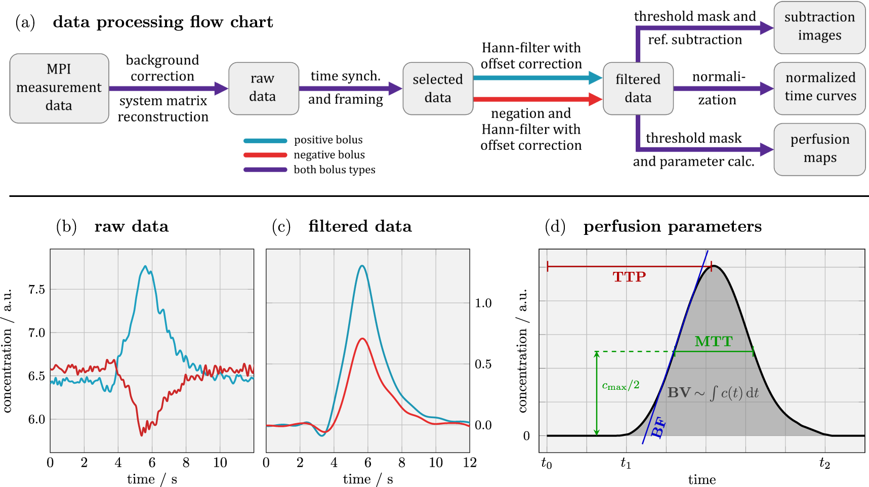
The entire data processing chain is displayed as a flow-chart in figure 2, along with data examples and parameter definitions. After reconstruction, the post processing includes time synchronization, data negation, Hann-filtering, voxel masking and lastly the perfusion parameter calculation. In the order of mention: the time is synchronized over all boli by selecting a time frame that starts with the injection (t₀), includes the first bolus (t₁ to t₂) and stops after the first passing (t = 12 s). This step ensures that only relevant data is processed later. For negative boli the concentration is inverted, so they can be processed identically to positive boli by the same code that works e.g. by using the maximum intensity. Afterwards, an appropriate filter type was chosen to smoothen the data for a more accurate peak detection and data interpolation, which also shifts the concentration offset to zero. To reject ringing artifacts, we avoided rectangular windows and selected a low-pass Hann-filter with a window-size of 10 samples. The Hann-filter is applied voxel-wise on the Fourier transformed temporal data. The last step before perfusion parameters are calculated is the determination of a threshold mask, which reduces image noise by excluding any voxel with an intensity lower than 6% of the maximum value for the selected time frame. The term 'raw data' refers to data reconstructed from the measurement signal before any processing, and 'filtered data' is a term for the final Hann-filtered data prior to post processing. This last step includes subtraction images, normalization and perfusion maps.

Zoom In Zoom Out Reset image size

Subtraction images. To visualize small changes in concentration, a pre-bolus reference is subtracted (pre contrast) from all following images (post contrast) to remove the native concentration, and consequently only changes in the concentration become visible (Hecht et al 2004). Dynamic subtraction images are based on the filtered data and calculated by subtracting with the identical spatial slice at t₀, that is before the administered bolus reaches the FOV.

Normalized images. By using a normalization, the time response of positive and negative boli can be overlaid e.g. to compare rise times or the shape of the bolus. To this end, the filtered data was used and normalization was applied to match maxima (in this graph only). The normalization is done via linear regression to match the maxima of the first peak without distorting the underlying time axis. Based on the linear model ${{\boldsymbol{c}}}_{t}^{\mathrm{bolus}\,1}={a}_{j}{{\boldsymbol{c}}}_{t}^{\mathrm{bolus}\,j}+{b}_{j}$ for all j ∈ {2,...,8} boli, a slope a_j and an offset correction b_j is determined for all time samples t, so each bolus can be mapped individually to one selected positive bolus (Zou et al 2003).

Perfusion images. In order to assess the feasibility of negative boli in perfusion imaging, calculations were performed on the filtered data for positive and negative boli using a threshold mask as described above and in figure 2(d). The data is not normalized for this calculation and the identical functions were used for positive and negative boli. The only difference is that negative boli are inverted before filtering. Perfusion maps are generated for TTP, rBF, rBV and MTT. The definition of individual perfusion parameters follows in section 2.4 below.

The following definitions are formulated continuously by using c_i (t), to provide a more general consideration. However, our data were processed using the discrete solution c_i,t .

TTP: the TTP is defined as the time elapsed between a chosen reference point (the bolus injection, here t₀) and the measured signal maximum of the first bolus passing (see figure 2(d)). The TTP $\in {{\mathbb{R}}}^{N}$ is calculated element-wise for all voxel i ∈ {1,...,N} via

$$\begin{eqnarray}&&{\mathrm{TTP}}_{i}=\arg \,{\max }_{t}\left(\,{c}_{i}(t)\right),\end{eqnarray} \tag{ 1 }$$

where c_i (t) is the concentration over time of the ith voxel (Fieselmann et al 2011).

PTT: the PTT is the time that a particle or blood cell needs to pass from the right to the left ventricle, therefore the average time that the blood circulates through the lung. It can be calculated by the difference of the TTPs of the ventricles (Deán-Ben et al 2015). In this work it is defined by a length of tube and the flow rate that was chosen to introduce a delay of about 1 s (see section 2.2).

rBF: the rBF equals the highest positive gradient in c_i (t)

$$\begin{eqnarray}&&{\mathrm{rBF}}_{i}=\arg \,{\max }_{t}\left(\,\displaystyle \frac{d}{{dt}}{c}_{i}(t)\,\right),\end{eqnarray} \tag{ 2 }$$

as shown in figure 2(d). A calculation for all voxels yields rBF $\in {{\mathbb{R}}}^{N}$. The BF and BV are calculated in a relative manner, due to a missing correct arterial input function.

rBV: the rBV can be derived from an element-wise evaluation of the AUC in the ith voxel, divided by the AUC in the artery to yield rBV $\in {{\mathbb{R}}}^{N}$. Therefore, the blood volume is proportional to the integral of c_i (t), divided by the integral of c_art(t) in the artery, over their respective time intervals [t₁, t₂] (see figure 2(d)), that mark the time the bolus needs for the first passing, as in

$$\begin{eqnarray}&&{\mathrm{rBV}}_{i}=\displaystyle \frac{{\int }_{{t}_{1}}^{{t}_{2}}{c}_{i}(t){dt}}{{\int }_{{t}_{1}}^{{t}_{2}}{c}_{\mathrm{art}}(t){dt}}\,.\end{eqnarray} \tag{ 3 }$$

MTT: the MTT is a measure of the average time that a particle or blood cell spends inside a vessel or organ. It is usually defined by the ratio of rBV to rBF or via the first moment of the AUC (Weisskoff et al 1993, Østergaard et al 1996), however, it strongly correlates with the full width at half maximum (FWHM) of the concentration peak (Kealey et al 2004, Østergaard 2005), especially for measurements with low tissue perfusion. To avoid error propagation due to inaccuracies in rBV and rBF (Weisskoff et al 1993, Østergaard et al 1996), we took the time interval FWHM as the MTT (Østergaard 2005), shown in figure 2(d).

Negative and positive boli are qualitatively compared by visual inspection of subtraction images, normalized data and perfusion maps. All these calculations are based on the filtered data set, but with an increasing computational effort in the mentioned order. The subtraction images reveal small changes in the concentration over time and require just the filtered time data and a threshold mask. Normalized images require a normalization step via linear regression and perfusion maps need to be processed according to section 2.4. All of these calculations were done for all boli, however, in the results only some boli and some perfusion maps are shown exemplarily. Positive boli are taken as the ground truth during comparison to negative boli in this work.

In figure 3(a), raw data of positive and negative boli in the left ventricle are shown, displaying several bolus passages over 100 s. The steady-state level increases slightly after each additional positive bolus (boli are administered alternately). Due to the relation of the chosen bolus concentration and initial baseline, peaks of negative boli are about 43% lower in the raw data.

Zoom In Zoom Out Reset image size

Below in figure 3(b), normalized curves based on filtered data of all 8 boli are shown for the right atrium and left ventricle. The normalized overlay of all 8 boli at the same location shows that curvature, shape and AUC coincide and are almost identical. On average, the FWHM is 12% smaller for negative boli in the right atrium and 5% smaller in the left ventricle, which predicts shorter rise times for negative boli. Boli were applied with identical procedure and alternatingly, hence a systematical fault in the setup is unlikely. An excessive low-pass filter setting would result in underestimating the bolus peak and equalize the FWHM difference between bolus types.

Dynamic time responses at different positions in the heart phantom are displayed in figure 4(a). The delay, in other words the transition times between different areas, and the shape of the bolus peak can be distinguished. We expected the width of the peak to increase with time, the AUC to remain constant, and the peak to be highest in the vena cava at the beginning. Limited resolution and unfortunate voxel spacing resulted in partial volume effects that led to locally lower concentrations compared with these expectations. The voxelsize of 2 × 2 × 1 mm³ is the lower limit for the represented resolution, but the smallest features of the 3D printed phantom were tubes with diameters below 2 mm, e.g. for the vena cava, aorta and pulmonary vessels. As a result, these concentrations are underestimated for both bolus types, which is visible here in the maxima and AUCs of the vena cava and aorta in figure 4(a).

Zoom In Zoom Out Reset image size

Below in figure 4(b), subtraction images are shown, suggesting that negative boli do not show significant deviation from the positive ground truth and dynamic imaging is possible. Each bolus can be seen to enter the right ventricle first, then passing through the pulmonary circuit and on to the left side of the heart. A small air bubble accumulated over the course of the experiments in the right ventricle in spite of all efforts to prevent air from entering the phantom. This caused a void in the images as no concentration changes occur except by movement of the bubble. Therefore, the bubble appears with zero intensity in subtraction images.

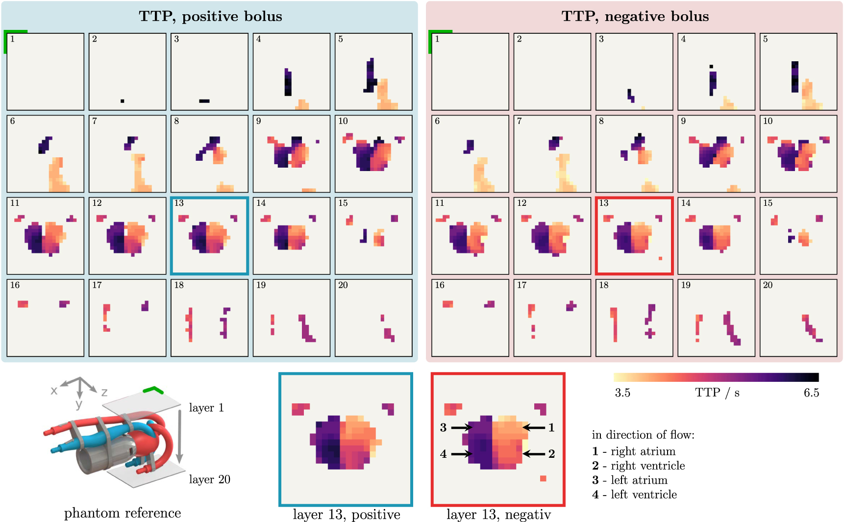
In figure 5, the TTP map is shown for a positive and a negative bolus, on the left and right, respectively. The top row shows the vena cava (blue) and the aorta (red), which are at the extremes of the colorbar, as they mark inlet and outlet of the heart phantom (compare to reference on bottom left). The bottom row shows the tubes of the pulmonary circuit (the return bend is outside the FOV), which are very similar in color shape due to the small time difference (PTT =1 s). The center of the heart phantom (layer 13) is enhanced to show that the 4 chambers of the heart are identifiable by slight differences in shading. The TTP was successfully obtained from a negative bolus and deviations between the two bolus types are low and in the same range of variations between administered boli of identical type. Note that the filtered data used in these results is not normalized, as this would impact the rBF, rBV, MTT, and the shape of the curve is therefore preserved.

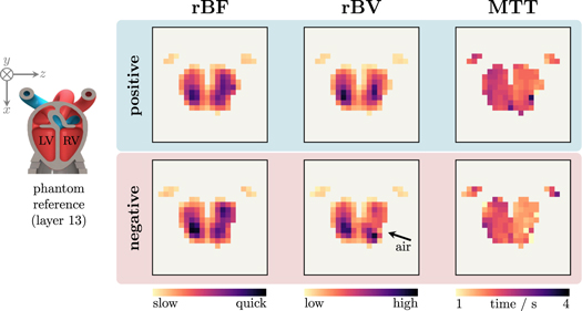
Zoom In Zoom Out Reset image size

Further perfusion parameters, namely the rBF, rBV and MTT, are shown in figure 6. Differences between the results of positive and negative bolus are small. The slightly darker tint of the negative rBF corresponds to the above mentioned difference in the FWHM, also visible in the data in figure 3(b). The same tendency can be seen in the MTT, which is a little shorter for negative boli. However, the MTT is generally around 2.5 s for both boli types and due to minor dispersion of the boli, the shading is darker in the left ventricle compared to the right ventricle, indicating that the bolus passed first through the right heart chamber and then through the left chamber. In the area of the pulmonary artery and the pulmonary vein, the actual blood flow is expected to be higher due to the smaller cross-section. The calculated blood flow shows the opposite due to the lower measured concentration. As already mentioned above with regard to figure 4(a), the local underestimation can be explained by partial volume effects and that the system matrix resolution is lower than the smallest vessels cross-section. This is consequently not a problem for the comparison between positive and negative boli, but a resolution-related limitation by the imaging system. Low resolution and partial volume effects prevented a correct definition of the arterial input function, consequently the BF and BV were calculated in a relative manner. Note that rBF and rBV are relative, however, they are scaled identically for positive and negative bolus types. These two images for one perfusion parameter are not normalized individually, therefore they refer to a common colormap for direct comparability.

Zoom In Zoom Out Reset image size

As mentioned in section 2.2, the tiny air pockets used to avoid dispersion during bolus preparation accumulated in the phantom, due to the position of the catheter just in front on the phantom. However, a bubble trap behind the catheter would have caused high dispersion of the bolus. Air also arose from cavitation in proximity to the pump, which prevented long experiments with more than 10 boli (around 5 min each).