
Abstract
Objective. Over the past years, convolutional neural networks based methods have dominated the field of medical image segmentation. But the main drawback of these methods is that they have difficulty representing long-range dependencies. Recently, the Transformer has demonstrated super performance in computer vision and has also been successfully applied to medical image segmentation because of the self-attention mechanism and long-range dependencies encoding on images. To the best of our knowledge, only a few works focus on cross-modalities of image segmentation using the Transformer. Hence, the main objective of this study was to design, propose and validate a deep learning method to extend the application of Transformer to multi-modality medical image segmentation. Approach. This paper proposes a novel automated multi-modal Transformer network termed AMTNet for 3D medical image segmentation. Especially, the network is a well-modeled U-shaped network architecture where many effective and significant changes have been made in the feature encoding, fusion, and decoding parts. The encoding part comprises 3D embedding, 3D multi-modal Transformer, and 3D Co-learn down-sampling blocks. Symmetrically, the 3D Transformer block, upsampling block, and 3D-expanding blocks are included in the decoding part. In addition, a Transformer-based adaptive channel interleaved Transformer feature fusion module is designed to fully fuse features of different modalities. Main results. We provide a comprehensive experimental analysis of the Prostate and BraTS2021 datasets. The results show that our method achieves an average DSC of 0.907 and 0.851 (0.734 for ET, 0.895 for TC, and 0.924 for WT) on these two datasets, respectively. These values show that AMTNet yielded significant improvements over the state-of-the-art segmentation networks. Significance. The proposed 3D segmentation network exploits complementary features of different modalities during the feature extraction process at multiple scales to increase the 3D feature representations and improve the segmentation efficiency. This powerful network enriches the research of the Transformer to multi-modal medical image segmentation.
Export citation and abstract BibTeX RIS

Original content from this work may be used under the terms of the Creative Commons Attribution 4.0 licence. Any further distribution of this work must maintain attribution to the author(s) and the title of the work, journal citation and DOI.
1. Introduction
Recently, deep learning networks (Simonyan and Zisserman 2014, Long et al 2015, He et al 2016) have dominated the field of computer vision. To a greater extent, automated image analysis approaches have surpassed the numerous models using manual feature extraction (Chuang et al 2006, Bosch et al 2007, Boiman et al 2008) in tasks such as image classification (Szegedy et al 2015, Huang et al 2017), semantic segmentation (Chen et al 2017, Zheng et al 2021), instance segmentation (Tian et al 2020, Yuan et al 2021), and object detection (Carion et al 2020, Sun et al 2021). Image segmentation, assigning semantic labels to each pixel in an image, is an essential task in computer vision. Currently, image segmentation's requirements for accuracy and reliability are escalating. In the environment of massive image data, relying on manual segmentation of image data becomes time-consuming, labor-intensive, and experience-dependent.
Medical image segmentation (Milletari et al 2016, Zhao et al 2018, Zheng et al 2018) is a vital task in computer-aided diagnosis and treatment (Yanase and Triantaphyllou 2019), which is a niche area of image segmentation. Medical image segmentation aims to outline regions of interest (organs or tissues) for pathological analysis, disease diagnosis, and the development of medical protocols. Earlier studies on medical image segmentation used manual or semi-automatic methods, such as thresholding (Moussallem et al 2012), graph-cut (Song et al 2013), and random walk (Liu et al 2018). However, purely manual segmentation is a highly subjective method, which strongly requires the physician's experience for guidance. The semi-automatic segmentation method has a narrow range of applications. It requires a manual setting of appropriate parameters or extraction of numerous processing features to ensure effective segmentation. In addition, this non-automated segmentation method is challenging to ensure the balance of segmentation efficiency and accuracy. With the improvement of computing power and the development of artificial intelligence (AI), more and more researches focus on automatic image segmentation.
Most studies on automatic medical image segmentation mainly focused on specific single-modality, such as computed tomography (CT), positron emission tomography (PET), or magnetic resonance imaging (MRI). Nowadays, the prevailing segmentation methods, such as UNET (Ronneberger et al 2015), have achieved outstanding results for single-modality segmentation and have built a symmetric network structure for efficient encoding and decoding. Today, most studies rely on this well-established segmentation structure. However, single-modality images do not fully reflect the proper pathological condition. In most cases, organs or lesion areas are visible in two different modalities, as shown in figures 1(a) and (b) in the first column. However, the other columns show that one can only locate the organ or lesion region only in one modality by the human vision.

Figure 1. Samples of single-modal and multi-modal images. (a) T2-weighted images (the first row), ADC scattering coefficients images (the second row), and the ground truth of the prostate (the third row). (b) FLAIR images (the first row), native T1 scan (the second row), and the ground truth of the brain tumor (the third row). Therefore, multi-modal scans can complement each other to obtain a better segmentation performance.
Download figure:
Standard image High-resolution imageWith the diversification of medical imaging devices and the complexity of pathological features, many clinical applications need to combine medical images from multiple modalities for analysis. Some existing research demonstrated complement each other can obtain a better analysis performance. These multi-modal methods help physicians measure the morphology and function of organs or tissues more accurately and develop more effective treatment plans. However, most existing single-modality networks are challenging to apply to multi-modal segmentation tasks directly. Therefore, a fast, effective and robust multi-modal segmentation method has excellent research importance.
Recently, most researchers have focused on applying convolutional neural networks (CNNs) in multi-modal medical image segmentation. Zhao proposed a multi-branch segmentation model (Zhao et al 2018) based on a fully convolutional network for segmenting non-small cell carcinomas in PET/CT images. Xu proposed a multi-modal segmentation method (Xu et al 2018) for PET/CT of whole-body bone lesions in multiple myeloma based on a cascaded network model (WNet). Alqazzaz proposed a multi-modal segmentation method (Alqazzaz et al 2019) for brain tumor MR image segmentation based on SegNet (Badrinarayanan et al 2017). Although these approaches contributed to the study of multi-modal image segmentation, they treat different modalities as two independent segmentation tasks. They do not effectively utilize the complementary information between the modalities. Moreover, the CNN-based method focuses excessively on images' local features and fails to capture the long-range spatial dependencies. And it concentrates almost exclusively on local feature relationships of images and ignores the global representation. Therefore, it is difficult for these methods to achieve the best segmentation results, especially for multi-modal image segmentation.
For multi-modal segmentation, we consider two of the thorniest issues: how to use complementary information from different modalities effectively and how to keep accurate global morphological and positional dependencies between organs or tissues. These are the keys to making multi-modal image segmentation more effective than single-modal image segmentation.
Fusing the features of two modalities can be divided into three class approaches. First, combine the two modal images into a single map before feature extraction. This simple approach can be directly segmented using the existing single-modal segmentation network. However, this will make the original information a significant loss, and also cannot fully utilize the complementary information of each modality. For example, Myronenko proposed a multi-modal 3D MRI tumor segmentation method based on encoder-decoder architecture (Myronenko 2018). Second, extract the features separately for both modality images, and fuse the results after obtaining the respective segmentation results. Similarly, this approach can be easily accomplished using a single-modal network but ignores the corresponding correlation between the two modalities during feature encoding. For example, Nie proposed a multi-modal segmentation method for segmenting the white matter (WM), gray matter (GM), and cerebrospinal fluid (CSF) of the infant's brain (Nie et al 2016). For each modality image, it trains one network only and then fuses their last feature for subsequent segmentation. In contrast, the third approach fuses the feature maps during the feature extraction process. Compared with the former two types of methods, it can extract the features of the respective modalities while considering the correspondence of the remaining modalities, which enables the model to learn more accurate feature information and can effectively improve segmentation accuracy. Fu introduces a multi-modal spatial attention module (MSAM) to automatically emphasize tumor-related regions and suppress distinct tumor regions (Fu et al 2021). Xue proposed a multi-modal segmentation strategy combining shared down-sampling of multi-scale features (Xue et al 2021). These studies show that different fusion methods get different segmentation results. Therefore, considering complementary information in the feature extraction process is the key to solving the multi-modal segmentation problem.
Transformer (Vaswani et al 2017) was conceived in natural language processing (NLP) for modeling long-range sequence-to-sequence tasks. Based on a multi-headed self-attention mechanism (MSA), it can model global contextual information and characterize global feature relationships more effectively. Recently, several works have introduced the Transformer to medical image segmentation tasks and achieved satisfactory results, especially for single-modal image segmentation. For example, Chen combined Transformer and CNNs to design TransUNet (Chen et al 2021) for medical image segmentation, which uses Transformer to extract global contextual information by encoding CNNs feature maps into contextual sequences. The UNETR proposed by Hatamizadeh uses the Transformer as an encoder to learn the sequence representation of the input quantities and efficiently capture the global multi-scale feature to achieve 3D medical image segmentation (Hatamizadeh et al 2022). Cao proposed Swin-Unet using a pure Transformer for medical image segmentation (Cao et al 2021). Valanarasu studied a gated axial-attention model that extends (Valanarasu et al 2021). Zhou proposed nnFormer, a powerful segmentation model with an interleaved architecture based on an empirical combination of Transformer and convolution (Zhou et al 2021).
Although these researches have effectively shown the feasibility of the Transformer model in medical image segmentation, there are still many challenges in applying the Transformer to multi-modal medical image segmentation. Sun proposed a multi-modal segmentation method based on Transformer and CNNs, which uses two parallel and independent paths to encode images from CNNs and Transformers, respectively (Sun et al 2021). Wang et al 2021 proposed a new encoder-decoder structure based on a novel TransBTS that utilizes the Transformer in a 3D CNN for brain tumor segmentation. However, these methods still do not fully consider the inter-modal correspondence and treat the two modalities as separate segmentation tasks. Moreover, due to the high computational cost required for the vision Transformer model, all existing Transformer-based segmentation methods are primarily based on 2D images and lack direct segmentation of 3D images. To the best of our knowledge, a few works have attempted to apply Transformer to multi-modal image segmentation among the existing studies.
This paper focuses on these problems and presents a robust 3D fusion segmentation network (AMTNet) that extends the Transformer for multi-modal medical image segmentation. The overall structure of our proposed method follows the typical U-shaped, but we have made many effective and significant changes in the feature encoding, fusion, and decoding parts. The encoding part comprises 3D embedding, 3D multi-modal Transformer, and 3D co-learn down-sampling blocks. The 3D Transformer block, upsampling block, and 3D-expanding blocks are included in the decoding part. In addition, there is a Transformer-based interleaved channel adaptive interleaved Transformer-based feature fusion module (AITF) designed to fully fuse features of different modalities. Comprehensive experiments demonstrate that AMTNet significantly improves the overall segmentation results, with the average DSC for the prostate being 0.907 and the BraTS2021 being 0.851, respectively. The main contributions can be summarized as follows:
- A novel automated Transformer-based multi-modal 3D medical segmentation network is proposed to extend the Transformer for multi-modal medical image segmentation.
- A novel channel interleaved AITF is proposed to effectively maintain multi-modal image features.
- Combining the advantages of Transformer and CNN allows our model to efficiently utilize global and local features.
In addition, we would like to mention that the present work is based on the improvement of our published conference paper (Tanel et al 2022). The specific points of improvement are the more detailed description of the proposed method. Specilally, we make an update to the network structure figure, detailing the design of effective fusion of multi-modal features, detail the role of designing restriction parameters inside the 3D-Transformer. For experiments, we change the random grouping of data to k-fold cross-validation for evaluation to reduce the influence of the specified testset on the results. In addition, the efficiency analysis with the comparison method is enhanced, including training time, model parameters, flops, inference time, etc. The remaining paper is organized as follows: section 2 provides an overview and detailed blocks of the proposed network. Section 3 presents comprehensive experiments and results. Finally, sections 4 and 5 show the discussion and conclusion.
2. Method
2.1. Overview
Figure 2 shows the proposed framework for multi-modal segmentation in medical images. The overall network structure of our proposed method follows the typical U-shaped.

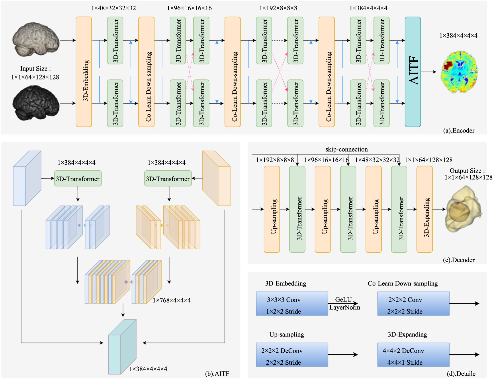
Figure 2. The architecture of the proposed AMTNet. (a) The encoding phase contains three modules, 3D-Embedding, 3D-Transformer, and Co-Learn Down-sampling. (b) Fusion module. (c) The decoding phase includes Up-sampling, 3D-Transformer, and 3D-Expanding modules. (d) Detailed design in AMTNet. It is worth noting that the input and output sizes shown in the figure are only the parameter settings of our model on the BraTS dataset (1 × 1 × 16 × 112 × 112 are setted on the Prostate dataset). It can be adjusted according to specific input data.
Download figure:
Standard image High-resolution imageFigures 2(a)–(c) show the practical and well-designed encoder, fusion, and decoder, respectively. The numbers in figure 2 represent the input image size and the number of channels at each stage. As shown in figure 2(a), the encoding part comprises three main blocks: 3D image embed block (3D-Embedding), 3D Transformer blocks for different modalities (3D-Transformer), and 3D Co-Learn Down-sampling (3D-CDS) block. In figure 2(c), the decoding part is similar to the encoding module. It includes the 3D Transformer block, Up-sampling block, and 3D-Expanding block for the output of the predicted image. Skip-connection joins the multi-scale features from the encoding part to the decoding part. In addition, there is a channel interleaved AITF in the U-shaped structure, as shown in figure 2(b), designed to fuse features of different modalities. Next, figure 2(d) describes the 3D-Embedding, 3D-CDS, AITF, and 3D-Expanding. Note that AITF can be considered as part of the encoder. The encoding part extracts multi-modal features from the input image, whereas the AITF module therein fuses the multi-modal features. These features are then up-sampled in the decoding section to output segmentation results at the same scale. Thus, this is a typical U-shaped structure.
2.2. Encoding
This subsection presents the detailed encoding part of the proposed segmentation network to exploit the multi-modal complementary features of different modalities. They are 3D-Embedding, 3D-Transformer, and 3D-Co-Learn Down-sampling.
2.2.1. 3D-embedding
In the first part of the network encoding phase, the leading role of the embedding layer is to divide the input image into small patches, similar to vision Transformer (VIT) (Dosovitskiy et al
2021). As mentioned before, we are concerned with multi-modal 3D medical image segmentation, so we must embed 3D images instead of 2D. Therefore, in this module, we convert the input 3D image  into a high-dimensional tensor
  where
where  represents the size of patch tokens and C represents the length of the sequence. As shown in figure 2(d), we extract features using sequential 3D convolution in the 3D-Embedding module, allowing for more detailed voxel-level patch encoding and facilitating accurate segmentation tasks. And after the convolution, GeLU (Hendrycks and Gimpel 2016) and layer normalization (LayerNorm) (Ba
et al
2016) are applied. In actual experiments, the size of the convolution in the 3D-Embedding can adjust precisely according to the input.
represents the size of patch tokens and C represents the length of the sequence. As shown in figure 2(d), we extract features using sequential 3D convolution in the 3D-Embedding module, allowing for more detailed voxel-level patch encoding and facilitating accurate segmentation tasks. And after the convolution, GeLU (Hendrycks and Gimpel 2016) and layer normalization (LayerNorm) (Ba
et al
2016) are applied. In actual experiments, the size of the convolution in the 3D-Embedding can adjust precisely according to the input.
2.2.2. 3D-Transformer
MSA is the Transformer's core, which calculates the similarity between patches. Generally, the MSA in VIT is designed for 2D images and does not apply to 3D medical images. It computes global similarity and brings a substantial computational effort. Many studied methods have demonstrated that calculating local similarity can reduce the computational effort and achieve better results with proper design (Liu et al 2021, Dong et al 2022). To effectively utilize the spatial properties of 3D medical images, we designed a 3D restricted multi-head self-attention (R-MSA) module, as shown in figure 3(b). It calculates the similarity between 3D patches and constrains the model to converge by the restricted parameters in our proposed method. It acts after two dot productions in the self-attention computation, thus restraining the abnormally large values of the feature maps of the dot product results caused by the different gray scales, window width, and window position of the medical images. Therefore, the method of learnable parameters makes the model learning fast and stable to facilitate the model convergence to some extent which has been demonstrated in section 4.2.

Figure 3. Detailed structure of the 3D-Transformer and R-MSA.
Download figure:
Standard image High-resolution imageIn addition to R-MSA, we also use local windows to reduce the computational effort in 3D-Transformer. Mainly, as shown in figure 3(a), we divided the 3D self-attention calculation process into two different parts by utilizing the multi-head mechanism (the size of the input image will determine whether to separate the third dimension or not). Our modal use half of the heads to calculate the self-attention of the horizontal 3D local window, while the remaining are used to calculate the vertical 3D local window. We concatenate the results of these two branches to get the complete 3D self-attention calculation results. Detailed calculation equations are given as follows.
Supposing that the 3D-Transformer input for the l
th
layer is  The 3D-qkv is calculated as in equation (1):

where q, k, and v represent the query, key, and value matrices designed in Transformer. The specific calculation of R-MSA is  where
where  and
and  are the vertical and horizontal attention given in equations (2) and (3):


where  and
and  are position encoding in both directions,
  and
and  are restricted parameters mentioned above. In the 3D-Transformer module, the last part after self-attention MLP is given as in equation (4).

where LayerNorm is a technique to normalize input data, which can effectively reduce the training time of the network, and MLP is used to enhance the nonlinear modeling capability of the model.
2.2.3. 3D-CDS
The advantage of the Transformer is to sense the global feature relationships of an image. However, preserving sensitivity to local features is still vital for fine-grained medical image segmentation. As mentioned before, CNNs are enabled to perceive local pixel relationships in an image. Therefore, we designed the 3D Co-Learn Down-sampling module (3D-CDS, as shown in the yellow block in figure 2(a)) to combine the advantage of Transformer and CNN. The detailed configuration is shown in figure 2(d). We introduced CNN to compensate for the perception of local features in our multi-modal Transformer network. This combination can reduce the feature map scale and the computational effort further. The information interaction between two modalities is strengthened by sharing parameters to enable different modality features to co-guide the model. Some misleading features are eliminated, thus realizing the multi-modal co-segmentation.
2.3. Adaptive channel interleaved Transformer feature fusion
AITF module is one of the cores of our multi-modal network. This module mainly comprises two parts: 3D-Transformer (for feature mapping) and channel interleaving fusion operation (for feature fusion).
In the mapping part, we use the 3D Transformer-based multi-modal feature mapping method. In the encoding stage, the model is able to learn the features of different modalities through the Transformer module that does not share the parameters and down-sample the feature map through the down-sampling module that shares the parameters. Before the AITF module, the feature maps generated by different modalities contain not only complementary features but also some misleading features. Therefore, in the AITF module, we need to eliminate the misleading features as much as possible and keep the complementary features. We design the Transformer module with shared parameters in the AITF module, which serves to unify the mapping of feature maps generated by different modalities, so as to eliminate some misleading features.
In the fusion part, we specially designed the fusion based on channel interleaving in order to effectively use complementary features and similar features. After the encoding part, feature maps generated in different modalities have certain variations, so the ordinary addition method cannot effectively express the importance and respective peculiarities of different modal features, and the channel concatenation approach cannot effectively express the association of similar features. In multi-modal imaging, different modal images scanned for the same body part share a high degree of feature similarity and complementary characteristics. This similarity is reflected in the region's location, shape, size, and other features to be segmented. Based on this, we assume that after mapping to the same feature space, the high-dimensional features of the two modalities obtained after the encoding stage have the same feature similarity in the same channel dimension. To prove this point, table 1 givens the similarity (using cosine similarity, Pearson similarity, and Manhattan distance) between features that are in the same and different channels, respectively. As shown in table 1, from the cosine similarity and Pearson similarity, we can see that the similarities of the feature maps of different modalities that are at the same channel are much higher than the feature maps between different channels. Also, the Manhattan distance between feature maps that are in the same channel is much lower. As shown in figure 4, the feature visualization results also support this claim. Therefore, in the AITF module, we design a new type of feature fusion based on channel interleaving. As shown in figure 2(b), we design the channel interleaved fusion by concatenating the features on the same channel from different feature maps and then downscaling the concatenated feature maps. Unlike the existing feature concatenation (where different feature maps are stitched together as a whole), we concate features in the same channel as a unit, thus preserving the similar features between different modes to a greater extent.
Table 1. The feature similarity of different channels.
| Different channel | Same channel | |
|---|---|---|
| Cosine | 0.4104 | 0.8166 |
| Pearson | 0.5548 | 0.8167 |
| Manhattan | 14.85 | 11.99 |

Figure 4. Feature similarity visualization for different channels (taking the BraTS dataset as an example). (a) and (b) are the feature map visualization results of the same channel of the two modal feature maps in AITF. (c) and (d) are the feature map visualization results of different channels of the two modal feature maps in AITF, respectively.
Download figure:
Standard image High-resolution imageIt works with the following flow: (1) Feed features from both modalities into the 3D-Transformer module with shared weights for feature mapping, so that feature maps with different characteristics remain in the same feature space and eliminate unfavourable features for segmentation. (2) Let the model learn the fusion weights for the two modal features to automatically allow the model to choose the importance of different modalities before channel concatenation. This fusion of channel interleaving preserves similar features in different modalities as much as possible and reduces misleading features' interference in segmentation. (3) Connect the original features input to the AITF module with the fused features in terms of residuals so that the fused features also retain the specificity features of their respective modalities, i.e. the complementary features we mentioned.
2.4. Decoding
For simplicity, the decoding part is set similarly to the encoding shown in figure 2(c). In decoding, the output fused with the features of the AITF module is gradually restored to the same scale as the input by the Up-sampling module. At this stage, our model combines the features from encoding with those from decoding by skip-connection. We also designed the 3D-Transformer module to map the features again to obtain more pleasing results. Finally, the model outputs the feature map as a segmentation result with the same scale as the input image through the 3D-Expanding module.
Our model outputs feature maps of different scales for depth supervision during the training phase. Specifically, besides the final output, two additional feature maps with different scales (or over two, which can adjust according to the actual experimental procedure) are obtained in the decoding stage to make the model converge more stably. Our model calculates the Cross-Entropy Loss (Lce) and Soft-Dice Loss (Ldice) for all outputs and then does a simple summation of these two losses, as shown in equation (5). Therefore, in this paper, the final training loss function is the sum of all the losses at three scales, as shown in equation (6).


where s, h and w are the voxel coordinates. In (5), wce and wdice are the weights for Cross-Entropy Loss and Logarithmic Soft-Dice Loss, which are hyperparameters. In (6), K represents different scales. λi is the weight for Lall.
3. Experiments and results
3.1. Dataset
The Prostate dataset (Simpson et al 2019) is a subset of the Medical Segmentation Decathlon 4 which contains image data of 10 different body parts. The target is segmenting the prostate central gland and peripheral zone and the segmentation challenge is the two adjoint regions with large inter-subject variations. The modalities are T2 and apparent diffusion coefficient (ADC). It contains 48 MRI studies provided by Radboud University reported in a previous segmentation study, of which 32 cases are annotated. The T2-weighted and voxel size of T2-weighted scans are 0.65 × 0.65 × 3.59 mm, and the ADC image is 2 × 2 × 4 mm. The image shape of both modalities is 320 × 320 × 20.
The BraTS2021 dataset (Menze et al 2014, Bakas et al 2017, kumar et al 2019, Baid et al 2017) is from the Brain Tumor Segmentation Challenge (BraTS) 5 . The challenge utilizes multi-institutional pre-operative baseline multi-parametric MRI scans and is divided into the training, validation, and testing datasets. It delivers multi-modal MRI scans of 2000 patients, of which 1251 cases are annotated. The dataset contains T1, T1Gd, T2, and T2-FLAIR volumes. Annotations are completed manually by experienced neuroradiologists. The voxel size of all sequences is 1 × 1 × 1 mm, and the image shape is 240 × 240 × 155. The labels include regions of GD-enhancing tumor (ET), the peritumoral edematous/invaded tissue (ED), and the necrotic tumor core (NCR).
These two datasets are representative data in the multi-modal study. We choose them to compare the strength and weaknesses of our model with existing models in this paper.
3.2. Implementation details
All experiments we conducted were based on Python 3.6, PyTorch 1.8.1, and Ubuntu 16.04. All training processes were performed using a single 12GB NVIDIA 2080Ti GPU.
3.2.1. Data processing
We performed pre-processing and data enhancement operations on the scans to facilitate the model training. In the data pre-processing, we resampled all the images uniformly to the same target spacing to prevent the discrepant information of the data itself from affecting the experiment. Meanwhile, we performed a series of enhancement operations on the training data: image rotation and scaling operations according to the same settings, as well as adding Gaussian noise, Gaussian blurring operations, adjusting brightness and contrast, and performing low-resolution simulation, gamma enhancement, and mirroring.
3.2.2. Network settings
In addition to the primary experimental environment configuration, table 2 reports some necessary configurations in AMTNet on Prostate and BraTS2021, such as the Crop size of the input network, Batch size, Embed_dim, the number of heads of MSA (No. heads), and the number of Transformers per layer (No. Transformer). It should be noted that there are different settings for Crop size and Embed_dim for these two datasets, because of the difference between these datasets.
Table 2. The network configuration of our model on Prostate and BraTS2021 datasets.
| Prostate | BraTS2021 | |
|---|---|---|
| Crop size | 112 × 112 × 16 | 128 × 128 × 64 |
| Batch size | 2 | 2 |
| Embed_dim | 96 | 48 |
| No. heads | [6, 12, 24, 12] | [6, 12, 24, 12] |
| No. Transformer | [2, 4, 7, 2] | [2, 4, 7, 2] |
3.2.3. Learning rate and optimizer
The initial learning rate init_lr was set to 0.01, and it decayed during training with the decay strategy shown in equation (7). The optimizer used SGD with momentum weight decay set to 0.9. The number of training epochs was 600 and the iteration of each epoch was 250.

3.3. Experiments results
In this paper, to validate the effectiveness of our method, we compare our method with some advanced multi-modal segmentation methods. They are MFNet (Zhou et al 2020), TCSM (Zhao et al 2018), MAML (Zhang et al 2021), WNet (Xu et al 2018), and MSAM (Fu et al 2021). MFNet independently used independent encoding paths to extract features from different modalities and then employed an attention mechanism to guide feature fusion for final tumor segmentation. TCSM used two V-Nets to extract PET and CT image features separately. They then summed the extracted features of different modalities to obtain segmentation results of lung cancer by 4-layer convolution. MAML used a novel mutual learning (ML) strategy for multi-modal liver tumor segmentation. It adaptively aggregates the features of different modalities in a learnable manner. It learns from each other through a pattern awareness (MA) module to extract features and commonalities between high-level representations of different modalities. WNet used a similar two-stage segmentation approach by first segmenting one modality to obtain a rough segmentation probability map and then superimposing it on another modality image before exact segmentation. MSAM introduced a MSAM that automatically learns to emphasize regions associated with tumors (spatial regions) and suppresses normal regions with high physiological uptake.
For a fair comparison, we used the same data preprocessing steps for all methods and the same data partitioning. And a 5-fold cross-validation was used for all experiments, and the average value was finally reported as the final results. Also, we quantitatively evaluated the segmentation results with evaluation metrics commonly used in medical image segmentation tasks, including Dice similarity coefficient (DSC), Jaccard similarity coefficient (Jaccard), relative volume difference (RVD), and 95% Hausdorff distance (HD95). For DSC and Jaccard, the bigger the value, the better the segmentation results. In particular, one of these metrics denotes perfect segmentation. However, for RVD and HD95, the smaller the value, the better the segmentation results (zero for these metrics denotes perfect segmentation). Tables 3 and 4 show these evaluation metrics, which compare our AMTNet with tested methods. The values in these tables are the means (standard deviations) of the different test methods on the prostate and BraTS2021 datasets and the best results are bolded.
Table 3. Experiment results on Prostate (the best results are bolded).
| Model | DSC | HD95 | Jaccard | RVD |
|---|---|---|---|---|
| MFNet | 0.791(0.004) | 6.087(0.374) | 0.685(0.029) | 0.301(0.007) |
| TCSM | 0.815(0.005) | 6.724(0.039) | 0.742(0.042) | 0.251(0.021) |
| MAML | 0.814(0.013) | 3.729(0.046) | 0.723(0.014) | 0.242(0.003) |
| WNet | 0.851(0.005) | 6.573(0.117) | 0.750(0.018) | 0.207(0.021) |
| MSAM | 0.875(0.011) | 3.679(0.111) | 0.787(0.009) | 0.156(0.022) |
| Ours | 0.907(0.004) | 3.172(0.079) | 0.823(0.010) | 0.136(0.016) |
Table 4. Experiments on BraTS2021 (the best results are bolded).
| Model | Region | DSC | HD95 | Jaccard | RVD |
|---|---|---|---|---|---|
| MFNet | ET | 0.566(0.020) | 9.416(0.353) | 0.402(0.052) | 0.544(0.052) |
| TC | 0.862(0.008) | 3.477(0.213) | 0.742(0.020) | 0.227(0.055) | |
| WT | 0.917(0.014) | 2.385(0.068) | 0.876(0.011) | 0.145(0.040) | |
| AVG | 0.782(0.005) | 5.093(0.121) | 0.673(0.012) | 0.227(0.015) | |
| TCSM | ET | 0.651(0.028) | 6.226(0.151) | 0.494(0.031) | 0.322(0.026) |
| TC | 0.864(0.017) | 4.322(0.492) | 0.717(0.045) | 0.219(0.047) | |
| WT | 0.917(0.015) | 3.001(0.024) | 0.887(0.018) | 0.141(0.032) | |
| AVG | 0.811(0.006) | 4.516(0.192) | 0.700(0.009) | 0.227(0.033) | |
| MAML | ET | 0.676(0.017) | 4.512(0.060) | 0.533(0.027) | 0.221(0.011) |
| TC | 0.870(0.012) | 3.497(0.251) | 0.851(0.026) | 0.253(0.029) | |
| WT | 0.911(0.016) | 2.280(0.212) | 0.846(0.024) | 0.227(0.034) | |
| AVG | 0.819(0.002) | 3.430(0.137) | 0.743(0.011) | 0.234(0.020) | |
| WNet | ET | 0.665(0.007) | 4.459(0.012) | 0.572(0.032) | 0.327(0.003) |
| TC | 0.885(0.002) | 3.432(0.209) | 0.819(0.006) | 0.225(0.012) | |
| WT | 0.910(0.020) | 2.263(0.308) | 0.853(0.030) | 0.162(0.021) | |
| AVG | 0.820(0.006) | 3.507(0.175) | 0.748(0.007) | 0.238(0.011) | |
| MSAM | ET | 0.692(0.016) | 3.841(0.112) | 0.565(0.037) | 0.368(0.013) |
| TC | 0.884(0.011) | 3.128(0.289) | 0.819(0.007) | 0.198(0.023) | |
| WT | 0.918(0.020) | 2.559(0.388) | 0.861(0.025) | 0.163(0.032) | |
| AVG | 0.832(0.006) | 3.176(0.184) | 0.749(0.007) | 0.243(0.021) | |
| Ours | ET | 0.734(0.022) | 3.928(0.029) | 0.569(0.023) | 0.225(0.003) |
| TC | 0.895(0.010) | 2.701(0.116) | 0.826(0.005) | 0.165(0.028) | |
| WT | 0.924(0.017) | 1.799(0.034) | 0.891(0.014) | 0.070(0.012) | |
| AVG | 0.851(0.002) | 2.809(0.049) | 0.762(0.005) | 0.154(0.013) |
3.3.1. Experiments on prostate
Firstly, we trained the overall prediction on the Prostate dataset for the whole prostate organ region. Quantitative and qualitative results about DSC, HD95, Jaccard, and RVD are shown in table 3 and figure 5.

Figure 5. Violin plot on Prostate. From (a) to (d) are the plot of DSC, Jaccard, HD95 and RVD for the MFNet, TCSM, MAML, WNET, MSAM, and our proposed method on Prostate.
Download figure:
Standard image High-resolution imageIn table 3, values in the table are the mean of the 5-fold cross-validated mean and standard deviation values (the number inside the parenthesis) of the different test methods, and the best results are bolded. Results show that our proposed AMTNet achieves the best mean DSC (0.907), HD95 (3.172), Jaccard (0.823), and RVD (0.136) on this dataset. And the standard deviations are the lowest among all the tested methods. As a comparison, the MSAM, WNet, MAML, TCSM, and MFNet methods had lower DSC than our proposed method by 3.2% to 11.6%.
Usually, the segmentation method's generalization in different scans is a paramount concern. This paper uses a violin plot to show the distribution of segmentation results. The violin plot is a hybrid of a box plot and a kernel density plot, which shows peaks and distribution in the collected data. Figure 5 shows a violin plot of the four metrics of all the tested methods on the Prostate dataset. In figure 5, the thick black bar in the middle of the plot represents the interquartile range, the thin black line extending from it means the data range with the maximum and minimum values at either end, and the white dots are the medians. The dots outside the line represent abnormal data. The subfigures show that our method leads in DSC, Jaccard, RVD, and HD95 metrics. In addition, our method showed the most concentrated distribution in all four metrics. In other words, our method offers the best stability for unseen scans.
To show the superiority of the proposed method from the training and validation stage, figure 6 shows the loss curves of our method and the compared methods.

Figure 6. DSC scores, training loss, and validation loss versus epoch for five comparison experiments performed with our proposed method during the training and validation phases on the Prostate dataset.
Download figure:
Standard image High-resolution imageChanges from the curves of these subfigures in figure 6 show that among the five comparison methods, the train_loss and val_loss of MFNet are relatively stable, but they drop slowly in the early stage of the training phase (the first 300 epochs). The train_loss of WNet can drop quickly and remain stable, but val_loss drops slowly in the first 150 epochs and fluctuates in the late stage. TCSM and MSAM train_loss and val_loss can drop rapidly, but val_loss fluctuates more. And both curves of MAML show a significant degree of fluctuation. All the curves of our method maintain a fast decline and can be stabilized quickly. These results indicate that our method has good feature learning ability, and the model is more stable in learning these scans.
3.3.2. Experiments on BraTS2021
MRI scans in BraTS2021 have four sequences: native T1-weighted images, post-contrast T1-weighted images (T1GD), T2-weighted images, and T2 fluid-attenuated inversion recovery images (T2-Flair). We can roughly divide them into two categories, T1 (native T1 and T1GD) and T2 (T2-weighted and T2-Flair). The T1 sequence can effectively show the anatomical structures, while the T2 sequence can well show the signals of tissue lesions. Among them, T1GD is bright in the area with blood vessels, while the tumor area without blood vessels will be dark, which is not conducive to the task of tumor segmentation. In contrast, the Flair sequence can show the tumor site circumference well and clearly show the puffy area compared with the T2 sequence. We selected native T1 and T2-Flair sequences for the tumor segmentation target to test our model. Unlike the Prostate dataset, the BraTS dataset has multiple regions to be segmented. Instead of predicting three mutually exclusive sub-regions corresponding to the segmentation labels, we predicted three overlapping areas: enhanced tumor (ET, original region), tumor core or TC (ET + NCR), and whole tumor or WT (ED + TC).
Table 4 shows the quantitative results of the 5-fold cross-validated mean and standard deviation values for ET, TC, and WT regions. The fourth row (AVG) in each tested methodizes the corresponding average values. In the table, the best mean results are bolded. Compared with these values. We can say that our proposed method gets the best DSC (0.851), HD95 (2.809), Jaccard (0.762), and RVD (0.154) in these regions. As a comparison, the MSAM, WNet, MAML, TCSM, and MFNet methods had lower DSC than our proposed method by 1.9% to 6.9%. In addition, our proposed method shows poor performance compared to the results on the Prostate. These may be the complexity of segmentation regions on BraTS2021.
Figures 7 and 8 show the violin plots for the four metrics and the loss curves of our method and the comparison method on the BraTS2021 dataset respectively.

Figure 7. Violin plot on BraTS2021. From (a) to (d) are the plot of DSC, Jaccard, HD95, and RVD for the MFNet, TCSM, MAML, WNET, MSAM, and our proposed method on BraTS2021.
Download figure:
Standard image High-resolution image
Figure 8. DSC scores, training loss, and validation loss versus epoch for five comparison experiments performed with our proposed method during the training and validation phases on the BraTS2021 dataset.
Download figure:
Standard image High-resolution imageIn the violin plots, the thick black bar in the middle of the graph represents the interquartile range, and the thin black line extending from it represents the data range, with the maximum and minimum values on either end, and the white dots as the median. Points outside the lines represent abnormal data which we think of them as poor segmentation results. These subfigures show that our method significantly outperforms the compared methods in all four metrics. These performances are similar to that of the Prostate dataset. All in all, the comprehensive results demonstrate its strong advantage in multi-modal image segmentation.
For the loss curves of our method and the comparison method, it is easy to see that MFNet can converge very quickly, but its segmentation ability is relatively low. In contrast, TCSM, MAML, WNet, and MSAM all show a greater degree of fluctuation than the Prostate dataset, and the final segmentation effect is lower than that of our proposed method. Although our method also shows some degree of flux, it is much smoother than the comparison method. Otherwise, it has a minor variation compared to the Prostate dataset, which also indicates the better adaptability of our proposed method.
3.4. Visualization
To visualize the segmentation results, we present some visualizations of the proposed method and the comparison method on the Prostate and BraTS2021 datasets in figures 9 and 10, respectively. In these figures, we superimpose the Ground Truth and the segmentation results on the original images. It is worth stating that Ground Truth is consistent in two modalities, so the observed differences between the segmentation results and Ground Truth are also consistent for the visualized images in different modalities.

Figure 9. Segmentation results for some cases of Prostate are superimposed on the two modalities separately. The first column shows the original image, the second column shows the ground truth, and the remaining columns show the segmentation results of the comparison method and our proposed method (the segmentation regions are marked in red).
Download figure:
Standard image High-resolution image
Figure 10. Segmentation results of some cases on BraTS2021 superimposed on two modalities. The first column is the original image, the second column is the ground truth, and the remaining columns are the segmentation results of the comparison method and our proposed method (ET, ED, and NCR regions are marked in yellow, brown, and green).
Download figure:
Standard image High-resolution image
As shown in figure 9, we superimposed the segmentation results on the T2-weighted image and the ADC image on the Prostate dataset, respectively. We present Ground Truth as a green contour line in the segmentation results, and the orange area represents the segmentation results. We show the segmentation results for two cases in total, in the first and second rows (case 1) and the third and fourth rows (case 2) in figure 8. The first row of each case is the T2-weighted image and the second row is the ADC image. From the figure, it can be seen that in the segmentation of case 1, the results of WNet, TCSM, and MAML are significantly smaller than Ground Truth. MFNet and MSAM are closer to Ground Truth, but their edges are not smooth, and overall, they are more irregular than Ground Truth. Although our method differs from Ground Truth in the proper segmentation, our segmentation results are more regular, complete, and smoother contours. In the segmentation of Case 2, when the region to be segmented is tiny, the segmentation results of all methods except MFNet are larger than Ground Truth. Our method has the slightest difference among them and has the most complete and regular overall shape. These show that our proposed method does well in segmenting the larger (case 1) and smaller (case 2) regions, showing the stability and effectiveness of the method.
As shown in figure 10, on the BraTS dataset, we superimposed the segmentation results on the T1 image and the Flair image, respectively. We mark the segmentation regions ET, ED and NCR in yellow, brown, and green, respectively. Similarly, we show the segmentation results on two cases, the first and second row of case 1 and the third and fourth row of case 2 in figure 10. The first row of each case is T1, and the second row is Flair. From the figure, we can see that for case 1, MFNet barely segmented the NCR region correctly. The NCR regions segmented by WNet and TCSM show a very irregular shape. Similarly, our method also segmented the NCR region slightly less than Ground Truth but presented a more regular shape. Furthermore, for the ED and ET regions, all methods segment better. For case 2, MFNet also appears to fail to segment correctly when the NCR presents irregularities and has holes. WNet segmentation results are significantly smaller than Ground Truth. The segmentation results of TCSM, MAML, and MSAM are similar to Ground Truth, but there are large differences in details, and the irregularities and holes appearing in them are not presented. While our method restores them to the maximum extent. It can be seen that our method is effective in segmenting both regular and irregular segmentation regions.
3.5. Computation efficiency analysis
To perform a proper comparison of computation efficiency between our proposed method and the comparison methods, in table 5, we report the training time (per epoch), the number of parameters of the model, and the FLOPs for all methods.
Table 5. Computation efficiency analysis.
| Model | Parameters (M) | FLOPs (G) | Training Time (S) |
|---|---|---|---|
| MFNet | 8.06 | 9 | 80 |
| TCSM | 62.05 | 1031 | 140 |
| MAML | 61.79 | 766 | 125 |
| WNet | 7 | 286 | 90 |
| MSAM | 18 | 2129 | 100 |
| Ours | 10.9 | 23 | 150 |
It can be seen from the table that although our proposed method has the longest training time, the number of model parameters and FLOPs maintain a more balanced level. It should be noted that the inference time per case is relatively consistent for all methods, ranging from 2 to 3 s.
4. Discussion
Recently, most studies on automatic medical image segmentation mainly focused on specific single modalities. But single-modality images do not fully reflect the proper pathological condition. With the diversification of medical imaging devices and the complexity of pathological features, many clinical applications need to combine medical images from multiple modalities for analysis. Some existing research demonstrated complement each other can obtain a better analysis performance. However, most existing single-modality networks are challenging to apply to multi-modal segmentation tasks directly. Existing CNN-based methods have swept around the world. They only concentrate almost exclusively on local feature relationships of images and ignore the global representation. It is difficult for these methods to achieve the best segmentation results, especially for multi-modal image segmentation.
In the past two years, Transformer was conceived in NLP for modeling long-range sequence-to-sequence tasks. It can model global contextual information and characterize global feature relationships more effectively. Several works have introduced the Transformer to medical image segmentation tasks and achieved satisfactory results, especially for single-modal image segmentation. However, due to the high computational cost required for the vision Transformer model, all existing Transformer-based segmentation methods are primarily based on 2D images and lack direct segmentation of 3D medical images.
To the best of our knowledge, a few works have attempted to apply Transformer to multi-modal medical image segmentation among the existing studies. For multi-modal segmentation, we consider how to use complementary information from different modalities effectively and how to keep accurate global morphological and positional dependencies between organs or tissues. These are the keys to making multi-modal image segmentation more effective than single-modal image segmentation. Therefore, we present a robust 3D fusion segmentation network (AMTNet) that extends the Transformer for multi-modal medical image segmentation. The AITF module and R-MSA are the most central parts of our proposed method to handle the two concerns mentioned above.
4.1. Importance of the AITF
The AIFT module plays a role in feature fusion in three main aspects to achieve higher accuracy of feature correlation: (1) Mapping the feature maps from two modalities in the same way so that they exist with the same feature space. (2) Learning parameters to adjust the fusion weights of the two modal features and allow the model to choose a more favorable combination for the final segmentation. (3) Integrating corresponding features channel-wise to allow the same feature channels to be stitched together. Since the two modal images are highly similar in morphology as a whole and the locations of the regions to be segmented are similar, they contain more similar features in addition to the complementary characteristics of the two modal features in the same channel dimension.
To demonstrate the contribution of the AITF module to accurate segmentation, we conducted relevant experiments. UNETR and nnFormer are two current advanced Transformer-based 3D medical image segmentation networks. However, both of them are single-modality segmentation methods. We have used our proposed AITF module for the fusion of feature maps of these two encoding networks by constructing two encoding network parts (which can be understood as replicating their single encoding module into two encoding modules). Then the decoding part keeps the original network unchanged, and the final segmentation results are shown in table 6. We also conducted experiments using 5-fold cross-validation on the two datasets, and the results in the table show the average DSC values of UNETR and nnFormer plus the added value of the AITF module. The adding values indicate the change in the AITF module compared to the fusion using the simple feature summation approach. The increased values indicate that the AITF module is effective in improving segmentation accuracy, i.e. boost improves by 2.1% (UNETR) and 2.3% (nnFormer) on the Prostate dataset and by 3.1% (UNETR) and 1.9% (nnFormer) on the BraTS2021 dataset.
Table 6. Experimentation of the AITF module on improving segmentation results.
| Datasets | Region | UNETR + AITF | nnFormer + AITF | Ours |
|---|---|---|---|---|
| Prostate | AVG | 0.849 + 0.021 | 0.862 + 0.023 | 0.907 |
| BraTS2021 | ET | 0.637 + 0.042 | 0.682 + 0.099 | 0.734 |
| TC | 0.843 + 0.029 | 0.871 + 0.036 | 0.895 | |
| WT | 0.917 + 0.019 | 0.921 + 0.011 | 0.924 | |
| AVG | 0.799 + 0.031 | 0.825 + 0.019 | 0.851 |
4.2. Validity of the restricted parameters
In image segmentation, the vision Transformer has established a long-range dependence on features through a MSA, which has led to good results for the corresponding downstream tasks. However, applying the MSA mechanism intact to medical image processing has the problem that medical images present much larger intensity values than natural images. In such a case, the attention computed by the MSA mechanism will have some extreme outliers, which may interfere with the model's learning of features. Although we can first address the image grayscale range by preprocessing the images, this will reduce the model's generalizability which makes it necessary for the model to make corresponding adjustments to specific datasets. Therefore, we propose the R-MSA mechanism with restricted parameters based on establishing a unified set of pre-processing processes. As shown in figure 3(b), the R-MSA mechanism constrains the computation of attention by adding two learnable parameters,  and
and  to the original MSA mechanism process, thus allowing the model not to be disturbed by outliers and thus enhancing the model generalization capability. We conducted ablation experiments on two parameters,
  and
and  in the 3D-Transformer model. As shown in table 7, the accuracy of our model decreases in the absence of these two parameters. In addition, we observe that without these two restrictive parameters, the training and validation losses of the model drop more slowly, requiring more than 150 epochs to drop below 0.2, a delay of 50 epochs compared to the case with these two parameters. Also, the model stabilization time is delayed by about 50 epochs.
Table 7. Experiment results with the significance of  and
and 
| Datasets | Region | Without two parameters | Ours |
|---|---|---|---|
| Prostate | AVG | 0.896 | 0.907 |
| BraTS2021 | ET | 0.731 | 0.734 |
| TC | 0.879 | 0.895 | |
| WT | 0.916 | 0.924 | |
| AVG | 0.842 | 0.851 |
5. Conclusions
This paper investigates a novel Transformer-based 3D segmentation network for multi-modal medical image segmentation. The method is implemented based on a U-shaped structure to exploit the complementary features of different modalities. This proposed network consists of 3D-Embedding blocks, 3D-Transformer blocks for different modalities, a shared 3D co-learning downsampling block (3D-CDS), and a channel adaptive interleaved Transformer feature fusion module (AITF), which helps to eliminate misleading feature information of different modalities and combine complementary information for cooperative segmentation. Extensive experiments have confirmed its effectiveness. However, our approach also has some limitations: all multi-modal data used in this work are registered as sharing the same annotation and cannot yet be used for multi-modal data with different annotations. Another limitation is that it is easy to produce over or under segmentation for tumors with low contrast in both modalities. The reason for this may be inadequate feature learning for regions that are fuzzy from the surrounding tissue. Our model currently has difficulty handling this challenging situation. In the future, we expect that by continuing to improve AMTNet, it will be able to handle multi-modal data with different annotations and segmentation problems at low contrast. We also expect that it will be useful for developing medically relevant tasks such as detection and disease classification.
Acknowledgments
We thank the anonymous reviewers for their careful reading of our manuscript and their many insightful comments and suggestions to improve the quality of this paper. This work was supported in part by the National Natural Science Foundation of China (Grant Nos. 61902046, 61901074 and 62076044) and the Science and Technology Research Program of Chongqing Municipal Education Commission (Grant Nos. KJZD-K202200606) and the Natural Science Foundation of Chongqing (Grant Nos. 2022NSCQ-MSX3746 and cstc2019jcyj-zdxm0011) and China Postdoctoral Science Foundation (Grant No. 2021M693771) and Chongqing postgraduates innovation project (CYS21310).