

Abstract
Objective. Transit in vivo dosimetry methods monitor that the dose distribution is delivered as planned. However, they have a limited ability to identify and to quantify the cause of a given disagreement, especially those caused by position errors. This paper describes a proof of concept of a simple in vivo technique to infer a position error from a transit portal image (TPI). Approach. For a given treatment field, the impact of a position error is modeled as a perturbation of the corresponding reference (unperturbed) TPI. The perturbation model determines the patient translation, described by a shift vector, by comparing a given in vivo TPI to the corresponding reference TPI. Patient rotations can also be determined by applying this formalism to independent regions of interest over the patient. Eight treatment plans have been delivered to an anthropomorphic phantom under a large set of couch shifts (<15 mm) and rotations (<10°) to experimentally validate this technique, which we have named Transit-Guided Radiation Therapy (TGRT). Main results. The root mean squared error (RMSE) between the determined and the true shift magnitudes was 1.0/2.4/4.9 mm for true shifts ranging between 0–5/5–10/10–15 mm, respectively. The angular accuracy of the determined shift directions was 12° ± 14°. The RMSE between the determined and the true rotations was 0.5°. The TGRT technique decoupled translations and rotations satisfactorily. In 96% of the cases, the TGRT technique decreased the existing position error. The detection threshold of the TGRT technique was around 1 mm and it was nearly independent of the tumor site, delivery technique, beam energy or patient thickness. Significance. TGRT is a promising technique that not only provides reliable determinations of the position errors without increasing the required equipment, acquisition time or patient dose, but it also adds on-line correction capabilities to existing methods currently using TPIs.
Export citation and abstract BibTeX RIS
1. Introduction
The increasing complexity of radiotherapy treatments demands for efficient and reliable verifications of all the treatment planning and delivery steps. In vivo dosimetry (IVD) is a widely recommended procedure that provides an end-to-end dose verification approach (The Royal College of Radiologists et al 2008, Olaciregui-Ruiz et al 2020a). Electronic Portal Imaging Devices (EPIDs) have experienced an increasing interest as transit IVD detectors for their availability, simple setup, digital format, high resolution, and improved dosimetric characteristics (van Elmpt et al 2008). There are two major approaches for EPID-based IVD. The first approach (or forward approach) compares the transit portal images (TPIs) to a set of reference TPIs used for constancy checks (McCurdy and Pistorius 2000, Bedford et al 2014, Hsieh et al 2017, Bawazeer et al 2018). The major drawback of this approach is that the dose in the patient is not calculated. Therefore, these methods have a limited ability to identify the specific cause of a given dose difference at the EPID plane and to quantify its clinical impact. The second approach is based on back-projecting the TPIs to provide a planar (2D) or a volumetric (3D) dose reconstruction within the patient that, contrary to the 2D comparison at the EPID level, can be directly compared with the dose distribution calculated by the treatment planning system. Back-projection algorithms constitute the most complete transit IVD approach to date (Louwe et al 2003, Wendling et al 2006, Wendling et al 2009, Bojechko and Ford 2015, Mijnheer et al 2018, Olaciregui-Ruiz et al 2020b). Despite their sophistication, the ability to quantify patient-related changes is compromised because they calculate the dose on a reference patient anatomy where those errors may not be present (Louwe et al 2003, Wendling et al 2009, Bojechko and Ford 2015, Li et al 2019, Olaciregui-Ruiz et al 2020b). It is well known that the dose reconstruction is preferred to occur on the Cone-Beam CT (CBCT) scan where the inter-fraction component of the position error has been potentially corrected (Li et al 2019, Olaciregui-Ruiz et al 2020b) but, even in this setting, the dose reconstruction is still compromised by the intra-fraction component of the position error.
Setup positioning is among the most common source of errors in clinical practice (Bojechko et al 2015). Due to its potential clinical impact, the sensitivity to detect position errors has been investigated for the two major transit IVD approaches mentioned above. Detection thresholds between 4 mm and 20 mm (Bedford et al 2014, Hsieh et al 2017, Li et al 2019, Olaciregui-Ruiz et al 2020b), and even no detection at all (Bojechko and Ford 2015, Bawazeer et al 2018, Mijnheer et al 2018) have been reported for particular treatment site and technique combinations, which are unacceptable levels for modern clinical practices. In these studies, the gamma analysis is the most common method to compare the in vivo and the reference/planned data. While all studies have reported lower gamma passing rates for increasing position errors, most of them have concluded that gamma passing rates depended dramatically on the treatment plan, tumor site, delivery technique and tissue heterogeneities (Bojechko and Ford 2015, Bawazeer et al 2018). Therefore, a universal and reliable correlation between the gamma passing rate and the magnitude of the position error could not be established. These limitations are consistent with the lack of correlation between gamma passing rates and clinically relevant differences reported for pre-treatment verifications (Kruse 2010, Nelms et al 2011, Zhen et al 2011, Carrasco et al 2012, Stasi et al 2012, Chiavassa et al 2019).
This poor sensitivity to position errors is also confirmed by long-term studies on the effectiveness of the back-projection algorithms. In a study reporting 3 years of clinical experience, only 2 out of 35 errors for which a corrective action was taken corresponded to patient position errors (Mijnheer et al 2015). In a similar study reporting 4 years of clinical experience, the authors identified 17 deviations that gave rise to an intervention, but none of them corresponded to position errors (Mans et al 2010). In contrast, a study based on an institutional incident reporting system found that failure modes related to patient positioning accounted for 47.2% of the total of reported near-misses with a high-scoring severity index in photon external beam radiotherapy (Bojechko et al 2015). These results suggest that, even though the position errors are one of the most common errors in clinical practice, current back-projection methods do not detect this kind of errors effectively.
The forward approach has similar limitations. Most IVD commercial solutions are based on forward approaches and use gamma analysis for evaluation. However, a typical gamma analysis (for example, 3%–3 mm) is too coarse to detect the subtle integrated dose differences due to the shift-induced variations in patient transmission (Bedford et al 2014, Hsieh et al 2017). Even though stricter gamma criteria would increase their sensitivity, the gamma analysis cannot unambiguously identify, nor quantify, the specific cause of a given dose difference.
In recent years, artificial intelligence and deep learning techniques have experienced an increasing interest in radiotherapy. While many studies have focused on the evaluation of patient-specific quality assurance measurements to detect and quantify predefined types of linac errors (Nyflot et al 2019, Kimura et al 2020, Potter et al 2020, Kimura et al 2021), only one study has simulated an in vivo scenario including patient changes so far (Wolfs et al 2020). Therefore, and despite promising results, TPI-based deep learning solutions to monitor patient position are still lacking in a clinical setting.
In this paper we introduce a novel approach to infer the projection of a position error of the patient by comparing in vivo TPIs to reference TPIs acquired or calculated under reference setup positions. We have recourse to a perturbation formalism to develop a simple algorithm for quantifying the projection of the position error. Our method does not require additional EPID calibrations, it is fast and simple, and it has on-line correction capabilities. To the authors' knowledge, it is the first dedicated method that uses the TPIs to determine intra- or inter-fraction position errors with on-line correction capabilities. A proof of concept for the clinical implementation of this formalism, which we have named Transit-Guided Radiation Therapy (TGRT) technique, has been proposed and validated. In the clinical setting, the TGRT technique can enhance patient monitoring without additional imaging or dedicated equipment by providing on-line corrections after the delivery of each treatment field. Alternatively, it can be used to trigger further positional checks through standard Image-Guided Radiation Therapy (IGRT) or Surface-Guided Radiation Therapy (SGRT) procedures if a position error is detected. Finally, the TGRT technique can also enhance current EPID-based IVD methods (that can be run in parallel) by either providing information on the cause of discrepancy and allowing an intra-fraction correction or, in case of a back-projection methods, performing a more reliable dose reconstruction on a shifted CBCT according to the determined position error.
2. Methods
2.1. Notation and definitions
Figure 1 defines the reference frames used throughout this formalism. The following notation and definitions are assumed:
-
 where SDD and SID stand for source-to-detector and source-to-isocenter distance, respectively.
 - A position error of the patient is characterized by an overall shift given in the reference frame R. Alternatively, the shift vector can be defined in the reference frame C as
defined in R, denotes the projection of to the isocenter plane (z = SID). defined in R', denotes the projection of to the EPID plane (z = SDD). For relatively small shifts, and
- The anatomy of a patient is described by a mass density distribution where is given in R. stands for the mass density distribution free of position errors.
- The mass thickness crossed by a photon traveling between the focal spot F and a given pixel located at in R' is denoted by t(x', y'). t0(x', y') stands for the mass thickness free of position errors.
- A TPI is a radiological image T(x', y') of a treatment field transmitted through a patient and collected by an EPID. T0(x', y') stands for a reference TPI free of position errors. D(x', y') represents the direct portal image (DPI) that the EPID collects when both the patient and the table are absent. In this formalism, the units of T, T0 and D are arbitrary.
- t(x', y'), t0(x', y'), T(x', y'), T0(x', y') and D(x', y') are scalar fields defined in R'. From now on, the explicit dependency (x', y') will be omitted from the equations for the sake of clarity.


Figure 1. The reference frame R rotates jointly with the gantry keeping its origin on the radiation focal spot (F). The z axis corresponds to the beam central axis. The EPID lies at the z = SDD plane. The 2D reference frame R' is attached to the EPID defining the horizontal (x' = x) and vertical (y' = y) image axes and it is centered at the z axis of R. A reference frame C rotates jointly with the couch keeping its origin on the isocenter (ISO) which lies at the z = SID plane. C defines the lateral (LAT), longitudinal (LNG) and vertical (VRT) couch directions. Gantry and couch rotation angles are designed by g and c, respectively. C and R axes are parallel when c = g = 0. For c = 0, the gantry rotates around the LNG axis of C. For g = 0, the couch rotates around the z axis of R. A shift vector  is depicted at the isocenter. The radial line from F through the end of
  defines the transaxial projections of
  to the isocenter plane (
 ) and to the EPID plane (
 ). The polar (
 ) and the azimuthal (
 ) angles of that radial line, defined in R, are also depicted.
Download figure:
Standard image High-resolution image2.2. Perturbation formalism
Under a relatively small position error of the patient, a TPI can be approximated by a first-order Taylor expansion as

where  is the perturbation term linear in
  and
and  is a vector field defined in R'. The approach taken here is that, given a reference TPI T0 and a TPI T under an unknown shift
  a model for
  can be used to determine that shift.
2.2.1. Patient anatomy under a position error
The mass density distribution describing the patient under a position error is  Under a small shift, it can be approximated by a first-order Taylor expansion as

The mass thickness t is computed as the line integral of  along the radial line from F to a given EPID pixel as

where ρ = 0 outside the patient and where the polar ( ) and the azimuthal (
 ) angles in R are determined by the R'-coordinates of the pixel through

The mass thickness describing the patient under a position error is  Under a small shift, t can be approximated by a first-order Taylor expansion as

where the gradient operator is defined in R'. Note that the z-component of the shift sz is not relevant in this first-order approximation.
2.2.2. Model for the perturbation term
The scatter contribution on the TPI varies slowly with anatomy changes (McCurdy and Pistorius 2000, Vieira et al 2004) and, in the context of small shifts, an exponential attenuation of the primary beam of the type (Fielding et al 2002)

suffices to derive an operational model for the perturbation term of equation (1). The average mass attenuation coefficient μ is taken as a free scalar parameter of the model. More elaborate models for the functional (6) can be found elsewhere (Wendling et al 2009, Olaciregui-Ruiz et al 2020b). Under a small shift, the model (6) can be expanded using equation (5) as

where  and the first-order Taylor expansion
  for
for  has been used. Comparing with equation (1), the following model for
  is obtained:

The expressions (7)–(8) depend on quantities that are easily obtained in the clinical setting, namely:
- T0 is acquired, for each field, after an initial and correct setup position during the first treatment fraction. If available, T0 can also be obtained from a dedicated calculation algorithm using the planning CT or the daily CBCT.
- t0 is obtained using equation (3) from the planning CT or the daily CBCT.
- μ is obtained by fitting the model (6) to the set of data {T0, D, t0} for each field.
- D is obtained during the pre-treatment EPID-based verification of that field. Note that it must be acquired at the same (or corrected for) SDD than T0. If available, D can also be obtained from a dedicated calculation algorithm.
2.2.3. Determination of the shift projections
Given a reference TPI T0 and a TPI T under an unknown shift  the shift projection
  can be derived from equation (7) as

When applied to N pixels, the set of equations (9) becomes an overdetermined system of N linear equations of the type

where A is the (N × 2)-matrix of the coefficients and B is the (N × 1)-column matrix of the independent terms of the linear system. A non-weighted linear least squares fitting method yields (Lewis 1991)

2.2.4. Determination of the patient rotations
Despite patient rotations not being explicitly included in this formalism, a simple method to determine the rotations around the z axis based on the TGRT technique is also provided.
A rectangular grid is defined over T0, T,  and
and  covering the corresponding field size (see the example of figure 2). At first-order, the rotation described by a given rectangular region of interest (ROI) of the grid under a relatively small patient rotation of angle
  can be approximated by a local shift vector

where  is the center of the corresponding (i, j)-ROI and
  is the unit vector along the local shift vector.

Figure 2. The 5 × 5 grid used for the field g = 180° of the plan A (see table 1). The central ROI is centered at the z axis of R. The vector  is defined from the beam central axis to the center of the (i, j)-ROI (highlighted). The estimation
  is assigned to the center of the (i, j)-ROI. The rotation of the patient is denoted by ω.
Download figure:
Standard image High-resolution imageBy applying the TGRT technique at each ROI, a vectorial map  is obtained, and equation (12) can be inverted to provide a set of independent estimations of the rotation
  as
as

where: (i) the dot product with  has been applied to both sides of equation (12) to isolate ωij
; (ii) the definition of
has been applied to both sides of equation (12) to isolate ωij
; (ii) the definition of  has been used; and (iii) the cyclic property
  has been used. Provided that the projection of
  onto
onto  along
along  is simply
  the patient rotation can be determined as the average among ROIs

The general case of a translation combined with a rotation is straightforward. The global shift  must be first determined by applying the TGRT technique to the whole image and then it must be subtracted from each
  before applying equation (14).
2.3. Experimental validation
2.3.1. Plan preparation and delivery
A preliminary experimental validation of the proposed formalism was performed using an anthropomorphic phantom (RANDO). The phantom was scanned, and clinically representative targets and organs at risk were contoured on CT images using Eclipse v15.6 (Varian Medical Systems). Table 1 provides a description of the treatment plans used in this validation. For Intensity Modulated Radiation Therapy (IMRT) technique plans, inverse planning (Photon Optimizer v15.6) was used in combination with the sliding-window delivery technique. For both IMRT and 3D Conformal Radiation Therapy (3DCRT) plans, clinically representative dose distributions were calculated using the Anisotropic Analytical Algorithm v15.6.
Table 1. Description of the treatment plans used for validation. Tumor site, delivery technique, beam energy, number of fields and dose per fraction are provided. For Simultaneous Integrated Boost (SIB) approaches, the dose levels delivered to low and/or intermediate and/or high-risk target volumes are listed.
| Plan | Site | Technique | Energy (MV) | Fields | Dose/fx (Gy) |
|---|---|---|---|---|---|
| A | Head and neck (oropharynx) (SIB) | IMRT | 6 | 7 | 1.6, 1.8, 2.12 |
| B | Head and neck (cavum) (SIB) | IMRT | 6 | 7 | 1.6, 1.8, 2.12 |
| C | Brain | 3DCRT | 6, 10 | 4 | 2 |
| D | Breast (SIB) | IMRT | 6 | 5 | 2, 2.45 |
| E | Breast | IMRT | 6 | 7 | 2 |
| F | Breast | 3DCRT | 6, 10 | 3 | 2 |
| G | Breast | 3DCRT | 6, 15 | 4 | 2 |
| H | Rectum (SIB) | IMRT | 6 | 7 | 1.8, 2.016 |
All plans were delivered to the RANDO phantom using a TrueBeam v2.7 (with a aS1200 EPID) and a Clinac 2100 C/D (with a aS1000 EPID) both equipped with a Millennium 120 Multileaf Collimator (Varian Medical Systems). A reference TPI T0 was acquired in integrated mode for all fields by placing the EPID at SDD = 150 cm. Then, the couch top was shifted between fractions using the same set of couch shifts  for all the plans (the subscript 0 distinguishes the true shifts from the determined shifts). This set of couch shifts consisted of 24 random shifts (Gaussian-distributed random numbers, with μ = 0 and σ = 5, were used to generate the sLAT, sLNG and sVRT couch components in mm) and 60 shifts between ±10 mm in steps of 1 mm along the three axes. At each position, i.e. for each fraction, TPIs T were acquired for all fields. We finally removed the phantom and the couch to obtain the DPIs D for all fields.
TPIs T were also obtained for the field g = 180° of plan A under a set of pure couch rotations from c = 1° to c = 10° in steps of 1°. In addition, two arbitrary couch shifts with sLAT = –sLNG = 2 mm and sLAT = –sLNG = 4 mm were added to the couch angle c = 3° to assess the general case of a translation combined with a rotation.
2.3.2. Determination of the shift projections
The per-field mass thickness t0
was obtained from the planning CT using the equation (3) and the Eclipse Scripting Application Programming Interface v15.6. An in-house code (MATLAB v2015b, MathWorks) was developed to fit the free scalar parameter μ of the model (6) using a non-weighted least squares method to the set of data {T0, D, t0} for each field. A second MATLAB in-house code was developed to determine the shift projections  provided by equation (11) for all fields and shifts. A threshold of 10% was set to exclude out-of-field non-relevant dose regions of D, T0 and T. A field-specific threshold was set for t0 to crop the body outline, i.e. field regions tangential to the body edges and extending outside the body were also excluded.
As shown in figure 1, the connection between a true couch shift  in C and the same true shift
  in R is a rotation of couch angle c around the VRT axis of C,
  followed by a rotation of gantry angle g around the LNG axis of C,
  i.e.
i.e.

The equation (15) was used to transform the set of true couch shifts  to the corresponding set of true shift projections
  for all fields. The performance of the TGRT technique was studied by: (a) comparing the determined norms
  and the true norms
  (b) assessing the angles
  between
  and
and  defined as

and (c) assessing the distances d between  and
and  defined as

The detection threshold of our method was defined as the largest true shift magnitude  that yielded an unsafe
  for more than 50% of the data below that threshold
  meaning that a correction of
  would increase the current position error for most of the cases.
2.3.3. Determination of the patient rotations
The set of data T0,  and μ used in the previous section for the field g = 180° of plan A was reused for the determination of the patient rotations using equation (14) for all couch angles and for the general case of a translation combined with a rotation. Three grids of 3 × 3, 4 × 4 and 5 × 5 rectangular ROIs were defined to assess the impact of the grid size on the determination of a pure patient rotation. The central ROI for 3 × 3 and 5 × 5 grids was excluded from the average in equation (14) due to rij
= 0 for those ROIs. ROIs outside the cropped regions by the lower thresholds applied to D, T0, T and t0 were also excluded to avoid an ill-conditioned numerical problem as in the previous section.
and μ used in the previous section for the field g = 180° of plan A was reused for the determination of the patient rotations using equation (14) for all couch angles and for the general case of a translation combined with a rotation. Three grids of 3 × 3, 4 × 4 and 5 × 5 rectangular ROIs were defined to assess the impact of the grid size on the determination of a pure patient rotation. The central ROI for 3 × 3 and 5 × 5 grids was excluded from the average in equation (14) due to rij
= 0 for those ROIs. ROIs outside the cropped regions by the lower thresholds applied to D, T0, T and t0 were also excluded to avoid an ill-conditioned numerical problem as in the previous section.
3. Results
3.1. Determination of the shift projections
Figure 3(a) shows a high correlation between  and
and  (
( R2 = 0.87). The dispersion increased for increasing
  due to the first-order nature of the perturbation formalism. Indeed, the root mean squared error (RMSE) between
  and
and  was RMSE = 1.0 mm, 2.4 mm and 4.9 mm for
  ranging between 0–5 mm, 5–10 mm and 10–15 mm, respectively.
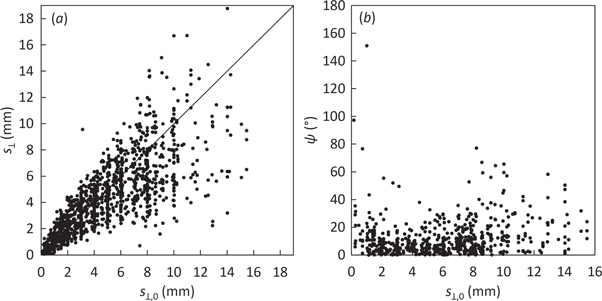
Figure 3. Scatter plots against the norms of the true shift projections  of: (a) the norms of the determined shift projections
  and (b) the angles ψ for all plans, fields and shifts. The solid line in (a) represents the identity.
Download figure:
Standard image High-resolution imageFigure 3(b) shows no correlation between ψ and  (
( R2 = 0.039). Figure 4(a) shows that the angular accuracy was better than 10°, 20° and 30° for 59%, 82% and 93% of the data, respectively, yielding an excellent angular accuracy of
  (mean ± 1σ). Only two points (0.2% of the data) yielded ψ > 90°. Such 'backward' shift determinations had minimal clinical impact because they corresponded to very small true shifts (0.2 and 1 mm).

Figure 4. Histograms of: (a) the angles ψ; and (b) the relative distances  for all plans, fields and shifts.
Download figure:
Standard image High-resolution imageThe distance d also increased for increasing 
 = 1.0 mm, 2.8 mm and 6.1 mm for
  ranging between 0–5 mm, 5–10 mm and 10–15 mm, respectively. The relative distance accuracy was
  (mean ± 1σ). Figure 4(b) shows that 96% of the data fulfilled
  (i.e. the
  correction would decrease the current position error). Interestingly, the 4% of the data with
  corresponded to
  < 3 mm, i.e. with a very reduced clinical impact.
Figure 5 shows the distribution of figure 4(b) stratified by validation plan. Table 2 shows that the corresponding relative distance accuracies  overlap within one standard deviation between plans. Table 2 also shows that the detection threshold was around 1 mm regardless of the plan, meaning that it has a very small dependence on the tumor site, delivery technique, beam energy or patient thickness. Note that for head and neck plans, with higher density variations than the remaining plans,
  could not be unambiguously determined because of the lack of sufficient experimental data for extremely small true shifts. Therefore, only upper limits of 0.3 mm and 0.2 mm could be set for plans A and B, respectively.

Figure 5. Boxplots stratified by validation plan of the relative distances  for all fields and shifts. Outliers (data at further distances than 1.5 times the interquartile range below and above the lower and upper quartile, respectively) are omitted for the sake of clarity.
Download figure:
Standard image High-resolution imageTable 2. Relative distance accuracy (mean ± 1σ.) and detection threshold for each plan and for all data together.
| Plan |

|
 (mm) (mm) | Plan |

|
 (mm) (mm) |
|---|---|---|---|---|---|
| A | 0.4 ± 0.2 | <0.3 | F | 0.6 ± 0.5 | 1.1 |
| B | 0.2 ± 0.2 | <0.2 | G | 0.4 ± 0.3 | 1.1 |
| C | 0.5 ± 0.4 | 1.5 | H | 0.4 ± 0.2 | 0.7 |
| D | 0.5 ± 0.4 | 1.3 | |||
| E | 0.3 ± 0.4 | 0.5 | All | 0.4 ± 0.3 | 0.5 |
3.2. Determination of the patient rotations
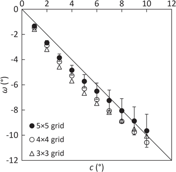
Figure 6 shows that finer grids slightly improved the determination of pure patient rotations compared to coarser grids (RMSE = 0.5°, 1.0° and 1.2° for 5 × 5, 4 × 4 and 3 × 3 grids, respectively). This result is not surprising, since a local shift vector  better represents a smaller ROI than a larger one. Statistical uncertainties (one standard deviation among ROIs) were approximately 10% for finer grids (5 × 5 and 4 × 4) and 20% for coarser grids (3 × 3). Using the 5 × 5 grid, table 3 shows that combined translations and rotations were satisfactorily decoupled. The angular RMSE (1.0°) and the average distance (
 = 1.6 mm) were compatible with the previous results.
Figure 6. Determination of the patient rotation ω against the true couch rotation c for each grid of ROIs. Error bars (±1σ among ROIs) are only displayed for the 5 × 5 grid for the sake of clarity. The solid line represents the identity. Note that clockwise (c > 0) couch rotations are seen as counterclockwise (ω < 0) patient rotations for the field g = 180°.
Download figure:
Standard image High-resolution image
Table 3. Determined rotation ω (mean ± 1σ among ROIs) and determined global shift projections  for a true couch rotation of c = 3° combined with three true couch shifts
  Note that clockwise (c > 0) couch rotations are seen as counterclockwise (ω < 0) patient rotations for the field g = 180°.
| sx,0 = sy,0 (mm) | ω (°) | sx (mm) | sy (mm) |
|---|---|---|---|
| 0 | –3.8 ± 0.9 | –0.5 | 0.0 |
| –2 | –3.0 ± 1.3 | –3.6 | –1.8 |
| –4 | –1.4 ± 3.0 | –6.6 | –3.7 |
4. Discussion
The proposed technique quantifies position errors with an accuracy of the shift magnitude that only depends on the shift magnitude itself (RMSE = 1.0 mm, 2.4 mm and 4.9 mm for  ranging between 0–5 mm, 5–10 mm and 10–15 mm, respectively) and with an excellent angular accuracy of 12° ± 14° which is independent of the shift magnitude. The detection threshold of our technique is approximately 1 mm, and it is nearly independent of the tumor site, delivery technique, beam energy or patient thickness, even for tumor sites with low density variations like brain or pelvis.
The performance of our method compared favourably to current transit IVD methods, which reported detection thresholds around 4 mm (Bedford et al 2014), 5 mm (Olaciregui-Ruiz et al 2020b), 10–20 mm (Hsieh et al 2017, Li et al 2019), and even no detection at all (Bojechko and Ford 2015, Bawazeer et al 2018, Mijnheer et al 2018), and strong dependences on tumor site, delivery technique and tissue heterogeneities (Bojechko and Ford 2015, Bawazeer et al 2018). The cited studies cover a wide range of scenarios: forward or back-projection approaches; measured or simulated/calculated TPIs; geometric/anthropomorphic phantom or patient datasets; 2%–2 mm or 3%–3 mm gamma metrics; head and neck, lung, esophagus, prostate, liver, spinal, brain, rectum or bladder treatment sites; and, finally, 3DCRT, IMRTor Volumetric Modulated Arc Therapy (VMAT) delivery techniques. Despite not all these combinations are addressed in our study, a different choice is not likely to affect the overall conclusions significantly.
Despite the rapid increase of artificial intelligence methods used in radiotherapy, only Wolfs et al (2020) have used convolutional neural networks to detect and identify the type and magnitude of treatment errors in an in vivo scenario. In this study, lung 3DCRT/VMAT plans and real patient datasets were used to predict TPIs under different types of simulated errors. The method classified the errors into three categories (anatomic changes, position errors or linac errors) with an accuracy of >95%. When classifying into magnitude subcategories (in the case of position errors, translations >1 cm versus translations <1 cm or rotations >0.5° versus rotations <0.5°) the accuracy decreased to >70%. As suggested by the authors, more detailed subcategories could impair the classification accuracy. Therefore, the ability of these methods to quantify the position errors is still limited.
A few studies have also recourse to the TPIs to extract the anatomical information of the patient for position checks. However, those algorithms require EPID calibrations using homogeneous phantoms of varying thicknesses depending on the patient diameter (Fielding et al 2002), and additional image matching algorithms to compare the anatomy images extracted from each TPI to the corresponding reference digital reconstruction radiography of that field (Fielding et al 2004). Our method provides a more efficient implementation of such TPI-based approaches.
Gamma analysis is a poorly conditioned comparison tool because a position error cannot be unambiguously estimated from the gamma passing rate value alone. This is because the gamma passing rate (or any other gamma-based statistical figure of merit) collapses relevant spatial information of the TPIs into a single number. The TGRT formalism overcomes the limitations of the gamma analysis by using a dedicated algorithm to directly quantify the position error from the TPI. A given position error can be readily determined after the collection of a TPI and therefore corrected before the delivery of the next treatment field, conferring on-line capabilities to the TGRT technique to correct both inter- and intra-fraction position errors. The main advantage of the TGRT technique is that it can be used at no cost, i.e. without the need of additional imaging, dose or time (as IGRT procedures) or dedicated equipment (as SGRT solutions). The TGRT technique may be especially suited for several clinical settings, for example, for palliative treatments with a high risk of intra-fraction patient motion, for deep-inspiration breath hold techniques, or for hypofractionated schemes where the intra-fraction monitoring is essential. For standard cases, the TGRT technique may be used to trigger additional position checks through standard IGRT procedures only if a position error is detected thus optimizing the treatment time and dose. However, the optimal implementation of the TGRT technique in the clinical setting is out of the scope of this study and it deserves a case-by-case analysis.
Position errors are one of the most frequent (Bojechko et al 2015) and difficult types of errors to catch by IVD methods and commercial solutions currently using TPIs (Mans et al 2010, Mijnheer et al 2015). The TGRT technique can be used in combination with current transit IVD methods, which can be run in parallel, to largely improve their performance. For example, the CBCT can be shifted and/or rotated accordingly to TGRT results and, therefore, more accurate transit estimations (for forward methods) or dose reconstructions (for back-projection algorithms) can be obtained.
The method to determine patient rotations provides a map of local shift vectors that can be used to assess anatomical variations of other types as well. For example, mandible or shoulder position checks or, possibly, most challenging internal deformation due to physiological processes can be addressed with this strategy. Our study has other potential improvements. Refinements of the model (6), including a quadratic term of t with a second free parameter accounting for spectral variations because of the flattering filter and the beam hardening in the patient, could improve the results (Fielding et al 2002, Fielding et al 2004, Wendling et al 2009, Olaciregui-Ruiz et al 2020b). Also, more elaborate methods than the current image-threshold approach to select the most relevant information of the TPIs; and the use of additional image processing techniques, would also be beneficial. A more comprehensive assessment addressing all these technique refinements is work in progress by using end-to-end Monte Carlo simulations (Baró et al 1995, Sempau et al 1997, Sempau et al 2011, Rodriguez et al 2013).
Our formalism could potentially be applied to VMAT plans as well, since VMAT plans can be interpreted as sequences of beams at different gantry angles. In VMAT techniques, only a small amount of monitor units is delivered at each control point, thus increasing the statistical noise of the corresponding TPI segment. Grouping neighboring segments would improve the noise, but as a result, angular information would be lost to some extent. Therefore, a balance between an adequate signal-to-noise ratio and sufficient angular resolution should also be explored.
5. Conclusions
A novel, simple and reliable EPID-based transit in vivo method for quantifying inter- and intra-fraction position errors based on a perturbation formalism has been presented. A proof of concept of a clinical implementation of this method, which we have named TGRT technique, has also been validated. The TGRT technique has the potential to drive the patient back to the target position by iteratively correcting for the determined position error after the delivery of each treatment field. Therefore, the TGRT technique is a promising on-line tool that can enhance patient position monitoring without any need for additional equipment, acquisition time or patient dose. More comprehensive studies to evaluate the performance of our technique for a wider range of clinical scenarios are work in progress.
Acknowledgments
The address of Artur Latorre-Musoll, Paula Delgado-Tapia and María Lizondo Gisbert when this work was carried out was: Servei de Radiofísica i Radioprotecció, Hospital de la Santa Creu i Sant Pau, Barcleona, Spain.
Josep Sempau thanks the Spanish Ministerio de Ciencia, Innovación y Universidades (projects FPA2017-83946-C2-2-P and PID2019-104714GB-C22) and the H2020 CONCERT European Joint Programme for the Integration of Radiation Protection Research (project 003-2017-PODIUM) for partial financial support.
The authors would like to thank Víctor Hernández Masgrau for his revision of the paper.
The authors have no relevant conflicts of interest to disclose.