
Abstract
Identifying tumour infiltration zones during tumour resection in order to excise as much tumour tissue as possible without damaging healthy brain tissue is still a major challenge in neurosurgery. The detection of tumour infiltrated regions so far requires histological analysis of biopsies taken from at expected tumour boundaries. The gold standard for histological analysis is the staining of thin cut specimen and the evaluation by a neuropathologist. This work presents a way to transfer the histological evaluation of a neuropathologist onto optical coherence tomography (OCT) images. OCT is a method suitable for real time in vivo imaging during neurosurgery however the images require processing for the tumour detection. The method demonstrated here enables the creation of a dataset which will be used for supervised learning in order to provide a better visualization of tumour infiltrated areas for the neurosurgeon. The created dataset contains labelled OCT images from two different OCT-systems (wavelength of 930 nm and 1300 nm). OCT images corresponding to the stained histological images were determined by shaping the sample, a controlled cutting process and a rigid transformation process between the OCT volumes based on their topological information. The histological labels were transferred onto the corresponding OCT images through a non-rigid transformation based on shape context features retrieved from the sample outline in the histological image and the OCT image. The accuracy of the registration was determined to be 200 ± 120 μm. The resulting dataset consists of 1248 labelled OCT images for each of the two OCT systems.
Export citation and abstract BibTeX RIS

Original content from this work may be used under the terms of the Creative Commons Attribution 4.0 licence. Any further distribution of this work must maintain attribution to the author(s) and the title of the work, journal citation and DOI.
1. Introduction
During the excision of a brain tumour the surgeon faces the challenge to remove as much malignant tissue as possible, but also to spare the benign brain tissue. The more tumorous tissue is removed, the higher is the survival rate of the patient, especially for gliomasurgery (Lacroix et al 2001). In order to achieve this, it is crucial for the surgeon to identify the transition zone from malignant to benign tissue. This task can also be aggravated by the infiltrative growth of of some tumours, e.g. glioblastoma multiforme, which results in an ill-defined transition zone (Thakkar et al 2014). Conventional imaging methods used during the tumour excision, like magnetic resonance imaging (MRI), fluorescence imaging or intraoperative ultrasound imaging are not able to resolve this transition zone properly and the resection quality heavily relies on the surgeon's experience. The current way to identify the transition zone is to use frozen section for fast analysis during operation or a retrospective histological analysis. Both methods result in either longer operation time or a delayed diagnosis, which can lead to new surgical intervention for the patient. Additionally they are spatially very inefficient due to the small size of the histological sample.
In recent years optical coherence tomography (OCT) has shown its potential to become an additional imaging method for the intra-operative detection of the tumour transition zone (Giese et al 2006, Böhringer et al 2009, Kut et al 2015, Yashin et al 2019). OCT is a contactless tomographical imaging method based on the interference of low coherent light (Fujimoto et al 2000, Drexler and Fujimoto 2008). The resulting images look similar to ultrasound images, but OCT can only resolve tissue in the depth of up to 2–3 mm. The advantage of OCT is the great trade-off between acquisition speed and spatial resolution. The resolution in OCT is usually between 5 and 30 μm and the images can be acquired in real-time. Because of these properties OCT is well established in ophthalmology (Adhi and Duker 2013).
The biggest limitation for the application of a supervised classification in order to identify tumour and its transition zones from healthy brain tissue is the creation of a ground truth dataset, which covers most of the tissue types, which could occur during the tumour excision. In past different research groups were able to separate highly tumorous tissue from healthy white matter, while other tissue types and inhomogeneous samples were not considered (Gesperger et al 2020, Juarez-Chambi et al 2020). On the other hand it was also shown, that more complex tissue compositions need to be included in the ground truth dataset, because the presence of necrosis in tumour infiltrated white matter changes the optical properties (Yashin et al 2019). Additionally grey matter needs to be included into the ground truth dataset. The optical properties of grey matter are very similar to tumour infiltrated white matter tissue, since both tissue types lack the highly scattering myelin fibres present in healthy white matter (Yashin et al 2019).
Another limitation for the creation of the dataset is the correlation of histological images with the OCT images due to the lack of structural features compared to e.g. retinal OCT images. This step is important for the consideration of heterogeneous tissue compositions and needs to be done automatically in order to be suitable for large numbers of images, which was not done by other research groups, because only homogeneous tissues were considered.
This work introduces a way to create a ground truth dataset for the supervised classification of human brain tumour, which accounts for the problems mentioned above. In order to account for different tissue types possibly present during tumour excision, a highly detailed labelling was applied to the histological data, which considered heterogeneous tissue combinations and differentiates different grades of tumour infiltration and other pathological tissue types, like edema or necrosis and distinguishes if the pathology is situated in grey and white matter. The histological labelling was then transferred onto corresponding OCT images using a shape based image registration approach, which also allows also the correlation of heterogeneous tissue compositions. Two different OCT systems with different optical properties (resolution, imaging wavelength) were used for data acquisition. Both OCT systems acquired OCT volumes of the same samples from the same region of interests. This will allow a comparison on which OCT parameters are essential for a good identification of tumour infiltrated tissue in human brain in the future. The process resulted in the creation of a ground truth dataset consisting of 1248 semantically labelled ex vivo OCT images from 17 patients acquired by two different OCT systems. In the future, the presented dataset will be used for differentiation of tumorous and healthy brain tissue based on OCT images
2. Materials and methods
2.1. OCT-systems
The data acquisition was performed with two OCT systems: a commercial off the shelf spectral domain (SD) OCT system (Callisto, Thorlabs Inc.) and a swept source (SS) OCT system (Optores GmbH, Germany). The core of this system consisted of a Fourier domain mode locked (FDML) laser with a central wavelength of 1310 nm and a spectral bandwidth of 110 nm (Huber et al 2006). The FDML technology allowed the acquisition of OCT A-scans with a rate of 1.6 MHz (Wieser et al 2010). An objective lens with a focal length of 54 mm and used a numerical aperture of 0.021 (LSM04, Thorlabs Inc.) was used during data acquisition. The lateral and axial resolution of the OCT systems were determined through point spread function (PSF) measurements, using the full width half maximum of nano particles dispersed in a non-scattering medium (OCT Resolution Validation Phantom, National Physical Laboratory) (Woolliams et al 2010). The results gave a lateral resolution of around 22μm and an axial resolution of 16 μm in air. The scan field of the system was set to 6 mm × 6 mm. The SD-OCT had a central wavelength of 930 nm and a spectral bandwidth of 127 nm. The system was equipped with an objective lens with a focal length of 36 mm and a numerical aperture of 0.051 (LSM03-BB, Thorlabs, Inc.). The lateral and axial PSF measurements showed a lateral and axial resolution of 5.2 μm and 4.9 μm in air. The field of view was 2 mm × 5.2 mm. The system was additionally equipped with a spectator camera, which allowed the acquisition of color images of a range of 12.8 mm × 9.6 mm. Both OCT systems were mounted on a movable rack system in order to be used in a separated room close to the operation theatre. The close distance of the OCT system to the tumour extraction assured that the sample was imaged as fresh as possible and that possible ex vivo tissue changes were kept to a minimum (Kiseleva et al 2019). During the data acquisition each system acquired one OCT volume scan and one en face image with the spectator camera was taken.
2.2. Sample preparation and data acquisition
21 patients participated in a clinical study in which several biopsies were excised from the patient from different locations (Study No.: 18-204, ethics committee University of Lübeck). 17 out the 21 patients were considered during this work, because complete datasets of the two OCT systems were available for these patients. Eight of these patients were diagnosed with glioblastoma multiforme (WHO IV), four with a glioma of grade WHO II or WHO III and the remaining five with metastasis (Arevalo et al 2017). 164 samples were excised in total for all 17 patients. The samples were extracted from tissue above the main tumour mass, the main tumour mass and from the border of the resection cavity after the resection was finished by the surgeon. The surgeon based his impression on the whitelight microscope and intraoperative information. Each sample was embedded into an agarose filled tissue cassette (figure 1, (e)). The tissue cassette had four imprints with varying sizes (3× 3 × 1, 4 × 4 × 2, 5 × 5 × 3 and 6 × 6 × 3 m3). The imprints were created with the help of a 3D printed mould as shown in figure 1, (a), which was pressed into the fluid agarose. During the data acquisition two mould designs were used (figure 2). The first one did only create cuboid imprints. An improved version added a flattened edge to the cuboid. This allowed a better identification of the sample orientation during the sample processing. After the agarose hardened, the mould was removed, leaving imprints behind. The imprints hold the tissue in a fixed position during data acquisition. The soft brain tissue adopts the shape of the imprint. Agarose was used as embedding medium, because it is easy to handle and does not interfere with the neuropathological processes.

Figure 1. 3D printed mould (a). Tissue cassette combined with mould (b). Box with prepared tissue cassettes, which was filled with agarose. Hot agarose pours into the tissue cassette and was then cooled off (c). Finished tissue cassette filled with agarose and visible cuboid imprints (d). Tissue cassette with sample (e).
Download figure:
Standard image High-resolution image
Figure 2. Top view white light image of the sample (a). The red square marks the field of view of the SD-OCT and is automatically generated. The lines define the location of taken OCT images and of the histological sections respectively. A histological section (b) and the labelled image (c) violet: vessel in white matter, olive: blood in white matter, cyan: blood in grey matter, blue white matter with tumour infiltration 0%–30% and pink: grey matter with 0% tumour infiltration correspond to the green line in the picture A. (d) Histological section of the sample shaped with second variation of the mould. The red arrow marks the flattened edge.
Download figure:
Standard image High-resolution imageEach OCT system acquired one OCT volume from the sample within 15 minutes after sample extraction. Afterwards the samples were fixated with a 4.5% formalin solution. The samples kept the shape of the imprint due to the fixation process. This allows to make assumptions about the sample size and shape, which was later used as a priori information during the registration processes. Ten histological sections were equidistantly (100 μm) cut from each sample. Location and orientation were defined prior on the top view white light image for each sample (cutting lines in figure 2). The histology sections were taken in the same orientation and plane like the OCT images. The straight edges of the cube shaped sample served as supporting planes during the cutting. Afterwards each sample was stained with hematoxylin and eosin (H&E). Each histological section was semantically segmented by a neuropathologist. The neuropathologist had 22 possible labels to choose from. The labels cover four different infiltration grades (0% (healthy tissue), 0%–30%, 30%–60% and >60% tumour infiltration), various other structures like edema, necrosis, vessel, blood, connective tissue, coagulation or cysts. The labels also differentiate if the tumour infiltration or structure is located in white matter or grey matter (cortex). The grade of tumour infiltration was subjectively chosen based on the experience of the neuropathologist. Figure 2 (c) shows an example of a segmentation done by the neuropathologist.
2.3. Work-flow and registration pipeline
This section covers the work-flow which transferred the histological information onto corresponding OCT images of the two OCT systems. The general registration pipeline is displayed in figure 3. The acquired data per sample consists of two OCT volumes (one per system), a white light image, which shows the top view of the sample, and ten labelled histological cuts. The position of the histological cuts are marked on the white light image. The first step of the process is to identify OCT images corresponding to the histological cuts. For this identification, the basic idea is to transfer the cutting lines, which represented the position of the histological images, onto the OCT volumes. The corresponding OCT images were then extracted along the transferred cutting lines. The second step is the transfer of the histological information onto the OCT images. This step consists of a non-rigid registration between the histological image and the OCT images based on the outer shape information of the sample, because inner structural features are usually not present. Finishing this work-flow results in a labelled dataset of OCT brain images acquired by two different OCT systems.
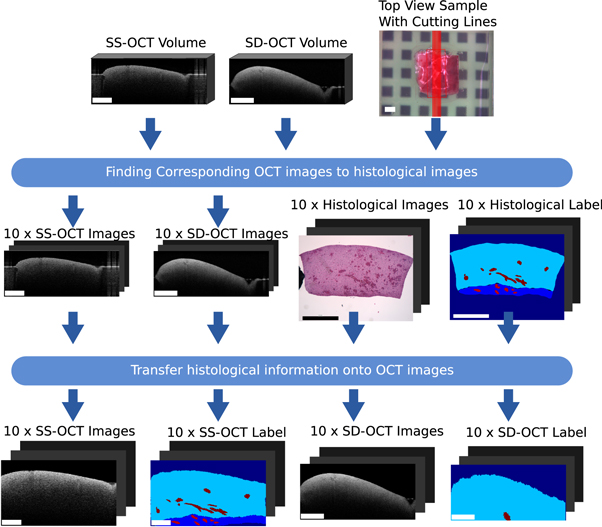
Figure 3. Overview of the work-flow of the transfer of histological label onto corresponding OCT images. The rectangle in the bottom left of each image has the length of 1 mm.
Download figure:
Standard image High-resolution image2.3.1. Finding OCT images corresponding to the histological cuts
This section describes the first step of the processing pipeline. It demonstrates how the cutting lines Cwl
= x, y were transferred from the white light image of the sample onto the OCT volumes, thereby determining the corresponding OCT images for each histological cut. Figure 4 shows the processing steps. The position of the cutting lines on the OCT volume of SD-OCT were known, since the white light image was acquired by this system. This means that the position of the OCT field of view and the spatial relations between the cutting lines and the field of view of the white light image were used to create a transformation matrix  , which considers translation, rotation and scaling. T1 was applied to the cutting lines Cwl
in order to transfer them onto the SD-OCT volume. This gained the position of the cutting lines on the SD-OCT volume Csd
.
, which considers translation, rotation and scaling. T1 was applied to the cutting lines Cwl
in order to transfer them onto the SD-OCT volume. This gained the position of the cutting lines on the SD-OCT volume Csd
.
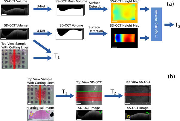
Figure 4. Overview of the work-flow to find OCT images corresponding to the histological images: (a) processing pipeline to determine the transformation matrices in order to transfer the cutting lines onto the OCT volumes. (b) Extraction of corresponding OCT images along the transferred cutting lines. The green and yellow markers show corresponding structural features. The rectangle in the bottom left of each image has the length of 1 mm.
Download figure:
Standard image High-resolution imageIn order to transfer the cutting lines Csd
onto the SS-OCT volume, an affine transformation  was calculated between the SD-OCT volume and the SS-OCT volume. T2 allows the transformation of Csd
onto the SS-OCT volume, resulting in the cutting lines Css
. The affine transformation matrix T2 considered rotation, translation and scaling between the two volumes. T2 was iteratively determined reducing the dissimilarity between topological height maps, which were generated from the OCT volumes (Maes et al
1996). The dissimilarity was computed through the mutual information and the optimization was done with the help of Powell's optimization method (Powell 1964). The topological height maps were used for the registration, because the height information is independent from the acquisition wavelength and intensity. The topological information was calculated from binary masks, which differentiate between tissue and agarose (foreground) and air (background). The mutual information was used because only relative height differences could be retrieved from the OCT images. This is because OCT can only measure distances with respect to the position of the reference arm of the OCT system. This means that there is a constant height shift between the height maps of one sample. The height value was defined as the depth value of the edge pixel between foreground and background.
was calculated between the SD-OCT volume and the SS-OCT volume. T2 allows the transformation of Csd
onto the SS-OCT volume, resulting in the cutting lines Css
. The affine transformation matrix T2 considered rotation, translation and scaling between the two volumes. T2 was iteratively determined reducing the dissimilarity between topological height maps, which were generated from the OCT volumes (Maes et al
1996). The dissimilarity was computed through the mutual information and the optimization was done with the help of Powell's optimization method (Powell 1964). The topological height maps were used for the registration, because the height information is independent from the acquisition wavelength and intensity. The topological information was calculated from binary masks, which differentiate between tissue and agarose (foreground) and air (background). The mutual information was used because only relative height differences could be retrieved from the OCT images. This is because OCT can only measure distances with respect to the position of the reference arm of the OCT system. This means that there is a constant height shift between the height maps of one sample. The height value was defined as the depth value of the edge pixel between foreground and background.
The binary masks were generated from each OCT volume by using a deep neural network with U-Net architecture (figure 5). The U-Net was introduced by Ronnenberger et al and is used for semantic image segmentation (Ronneberger et al
2015). The advantage of the neural network compared to usually used minimal path search algorithms is that it can adapt better to artefacts (e.g. reflections). The U-Net architecture used for this work was very close to the original publication, only the input and output size was changed to match the size of the OCT images, which had an input size of 516 × 1300 pixel. Each input image was extrapolated by mirroring to a size of 700 × 1484, so that the output size matches the original image before the padding. As a training dataset, 1700 (arbitrarily chosen) images from each OCT system were extracted from the OCT volumes of 80 different samples. A ground truth segmentation was created by manually segmenting the images into foreground and background. For the training the dataset was divided into training (80%) and test data (20%). 25% of the training data was used as validation data during the training. The split of the dataset was between the samples in order to assure that images from the same sample were only present in one sub-dataset to reduce overfitting. During each training step random data augmentation was applied to the OCT images. The data augmentation involved a random adjustment of the contrast and a random horizontal shift of the image content. This was done in order reduce the chance of overfitting and to improve the generalization of the U-Net. The training was performed for 300 epochs. For the optimization an Adam-optimizer with a learning rate of 0.000 001. The loss function was defined as the sum of the binary cross entropy Lce
and the dice loss Ld
(Ronneberger et al
2015, Milletari et al
2016, Taghanaki et al
2019). It combines the advantages of the dice loss to give valid results for imbalanced segmentations problems, where one class is under represented and the cross entropy, which focusses on the penalization of false positives and false negative segmentations (Taghanaki et al
2019). The cross entropy was calculated for each pixel of the OCT image, while the dice loss was determined as a scalar value for each image. So the loss function L combines local and global metrics. p(i) is the binary ground truth and  is the prediction between 0 and 1. N is the number of pixels in the mask, the pixel is defined by i.


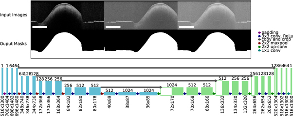
Figure 5. Overview of the configuration of the U-Net used to create the binary masks from OCT images. Examples of input OCT images with the used data augmentation and the corresponding output masks used to train the network (top). Architecture of the U-Net in order to process the OCT images. The rectangle in the bottom left of each image has the length of 1 mm.
Download figure:
Standard image High-resolution imageThe resulting affine transformation T2 was then applied to the cutting lines Csd of the SD-OCT to complete the transformation onto the SS-OCT. An example for a successful registration is shown in figure 4. The histological section and the corresponding OCT B-scans were extracted along the same 'cutting line'. The green and yellow marker show visible structural features, which can be seen in all three images. The overall surface contour also shows similarities between the images.
2.3.2. Label transfer from histology to the OCT images
This section deals with the second step of the workflow. It explains how the histological information in form of the delineated label was transferred onto the OCT images. The process will be described for the labels transfer onto the images of the SS-OCT images, but was analogue for the SD-OCT images. Figure 6 shows the processing pipeline of the label transfer.
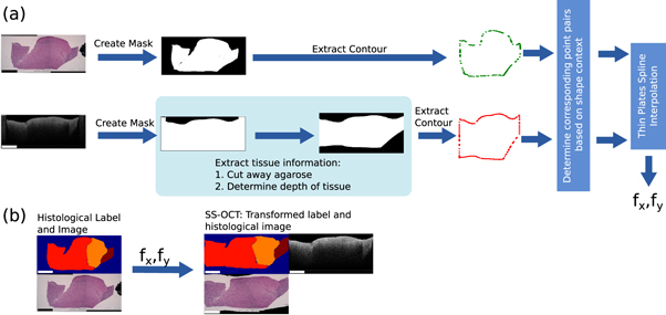
Figure 6. Overview of the work-flow to find transfer the histological information onto the OCT image: (a) Determination of the displacement fields T between the OCT image and histological image. (b) Transformation of the histological label and image onto the OCT image with the displacement fields T. The rectangle in the bottom left of each image has the length of 1 mm.
Download figure:
Standard image High-resolution image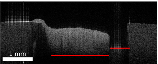
Figure 7. Depth of the agarose shape in the OCT B-scan varies with the axial position and thickness of the tissue due to differences in the refractive index along the depth axis.
Download figure:
Standard image High-resolution imageA transformation had to be determined for the transfer of the labels from the histology image onto the corresponding OCT image. The transformation is based on the outer shape of the sample. Due to the different image modalities and varying grade of details shown in the images, the use of intensity based features was not feasible. The outer shape of the tissue imprinted by the agarose hole is assumed to be similar in the OCT image and in the histological cut. The first part of the processing is the extraction of the tissue part from the histological image and the corresponding OCT image as binary mask which contain the information of the outer tissue shape. For the histological image the tissue was extracted based on the colour difference between the stained tissue and the white background. Locating and extracting the brain tissue in the OCT images took a few more steps: Each OCT image was processed through the already mentioned U-Net, which results in a binary mask. The columns of the mask were set to 0, if a column showed agarose in the original OCT image. The vertical margins were set manually by marking the left and right edge of the tissue in the OCT image, which was clearly distinguishable from the agarose. The pixel location of the bottom of the agarose imprint needed to be estimated, because the border between agarose and tissue was not visible due to the depth signal decay of the OCT image. This pixel location depends on the ratio of air and tissue. Since this ration changes over the OCT image, the location had to be determined for each image column. The axial pixel size Δs is scaled with the inverse refractive index of the medium n ( ). Figure 7 shows this effect unambiguously. If the agarose imprint is only filled with air (nair
= 1), the bottom of the agarose imprint appears higher in the OCT image whereas a composition of tissue (ntissue
> 1) appears lower.
). Figure 7 shows this effect unambiguously. If the agarose imprint is only filled with air (nair
= 1), the bottom of the agarose imprint appears higher in the OCT image whereas a composition of tissue (ntissue
> 1) appears lower.
The composition of air and tissue was determined from the binary mask. Since the composition of the brain tissue is unknown, it was assumed to have a constant refractive index of nt = 1.36 (Gottschalk 1992, Müller and Roggan 1995, Honda et al 2018). The actual depth d can be determined by the sum of all scaled pixel sizes:

Here z was defined as the axial pixel position within the image column. For each column of the binary mask pixels were set to 0 after the depth of the agarose imprint was reached. This results in a mask which marks the tissue content of the OCT image (figure 6).
After the extraction of the binary masks of the histology image and the OCT images, all masks were filtered by an edge filter in order to gain the mask outline, which essentially holds the outer shape information of the tissue. Each point of the mask outline has now a potential corresponding point on the other outline, which needs to be found in order to calculate the transformation between the two image modalities. For each point on an outline, a shape context feature was calculated (Belongie et al 2002). The shape context feature is a histogram-based descriptor, where the histogram describes the relative position of a point within a point cloud by a two dimensional histogram. In the first dimension the histogram bins describe the logarithmic spaced Euclidean distances log(r) from one point to all the other points of the silhouette. The logarithm was added in order to be more sensitive to close point position variations. Five bins were used from 0.125 to 2. Values smaller or bigger than the limits were assigned to the nearest bin. To achieve scale invariance, the Euclidean distance was normalized by the median distance between all the distances within one point cloud (Belongie et al 2002). The second dimension of the histogram describes the angle θ between the points, which was defined as the tangential angle between the point coordinates. Twelve bins were used ranging from 0 to 2π. To achieve some degree of rotational invariance, the angles were subtracted by the angle relative to the x-axis of the 1st principal component, which was calculated through the principal component analysis of the point cloud (Belongie and Malik 2000). The shape context features were determined for each point on the outlines. In order to identify the corresponding point pairs a linear assignment problem was solved based on the similarity of the feature histograms as described by Belongie et al (Belongie and Malik 2000).
The corresponding point pairs between two outlines were used to determine the transformation between the histological image  and
and  . An iterative thin plate spline interpolation approach was used for the determination in form of displacement fields
  and
and  (Bookstein 1989, Belongie and Malik 2000). The displacements in x and y direction were calculated between corresponding points pairs of the histological image Phist
and the OCT image POCT
, which were interpolated to a displacement fields using the thin plate spline interpolation. The displacement fields fx,y
were described by the following equation:
(Bookstein 1989, Belongie and Malik 2000). The displacements in x and y direction were calculated between corresponding points pairs of the histological image Phist
and the OCT image POCT
, which were interpolated to a displacement fields using the thin plate spline interpolation. The displacement fields fx,y
were described by the following equation:

By using the histological contour points Phist
as supporting points and the displacement fx
(xi
, yi
) or fy
(xi
, yi
) between the corresponding points pairs of Phist
and POCT
, equation (5) can be solved for variables a1, ax
, ay
and wi
as described in Bookstein (1989) in order to gain the displacement for all the pixels of Ihist
. U(r) is a kernel function, which was defined as  . The displacement fields were then applied to the coordinates of the histological image x and y in order to map them onto the OCT image coordinates
  and
and  .
.


The thin plate spline approach allowed the usage of a regularization parameter, which controls the stiffness of the transformation. The higher the regularization, the more the transformation resembles an affine transformation. Four iterations were used for the determination of the transformation. The regularization parameter was decreased with each iteration. The first iterations ensured an almost affine transformation for a general registration of the outlines, while the last iteration enabled an individual registration of the irregular outlines. The displacement fields from each iteration were then applied to the label of the histological section. Figure 6 shows an example of the transformation of the histological section onto the corresponding OCT image and the resulting transformed histological label.
3. Results
The presented pipeline was performed on 1630 histological images and their corresponding OCT images. In 75% of the cases the histological sample stayed in the shape given by the embedding process. These samples were then to transform the histological labels onto the corresponding OCT images. Examples of a successful transformation are shown in figure 8. For the remaining 25%, the sample changed its shape too much during the histological preparation (e.g. tearing of the tissue), which disabled usage of the shape information needed for the transformation. The evaluation of the U-Net, used for the creation of binary masks, was performed on the independent test data set. The test data set consisted of 342 OCT images. The test data set was processed with the U-Net and was compared against the ground truth segmentations by using the dice score (Dice 1945). The network achieved a dice score of 0.9970, which indicates that the U-Net adapted very well to the binary segmentation task. Additionally, the U-Net segmentation of background and foreground was compared to a graph search algorithm, which can be alternatively used for the creation of binary masks (Duan et al 2012). The test dataset was also used for this task. For both algorithms the tissue surface was extracted from the resulting binary masks. The absolute difference to the ground truth was calculated. The graph search algorithm achieved a median difference of 2.0 [1.0; 11.0] pixel, while the U-Net achieved a median difference of 0.0 [0.0; 1.0] pixel. The values in the square parentheses indicate the first and third quartile. The processing time of the U-Net was 0.2 s for one OCT image, while the graph search algorithm took around 30 s for one OCT image. In order to evaluate the registration process based on the OCT height maps (registration of the SD-OCT volume onto the SS-OCT volume), the top view intensity projections of the volumes were also put through the same registration process. The top view intensity projection, also called en face view, is usually used for visualization of the top view of an OCT volume V(x, y, z) and is defined as the mean intensity along the depth axis z

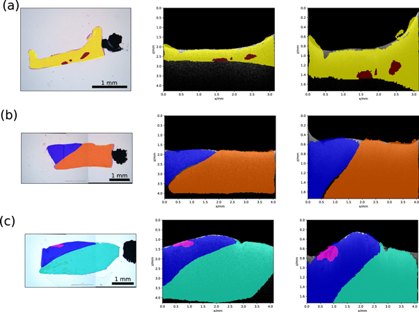
Figure 8. Transformation results for three exemplary samples: histological image and label (left), corresponding SS-OCT image and transferred label (centre) and SD-OCT image with transferred label. Meaning of the colors is as follows: yellow—white matter with 0% tumour infiltration, red—coagulation in white matter, blue—grey matter with 0% tumour infiltration, orange—edema in white matter, pink—blood in grey matter and cyan—white matter with 0%–30% tumour infiltration.
Download figure:
Standard image High-resolution image
The registration process was run again for the height maps and the en face images over 164 samples. For each registration the final value of the mutual information was saved. The mean mutual information for the registration of the height maps was 1.92 ± 0.59, while the mean mutual information for the registration with the en face images was 0.37 ± 0.25. The results show that the registration based on the height maps gave a higher mutual information value than the registration based on intensity information. This indicates that the registration with the height maps delivered a better registration result, because the mutual information increases with higher similarity between the images. The topological information of the sample was better suited for the registration in this case, because the intensity values of the homogeneous brain tissue did not show a lot of features, like vessels, which could have helped with an intensity based registration approach. The evaluation of the label transfer process was done with 30 manually chosen histological images and their corresponding OCT images from the two systems. The sample size for this analysis was rather low compared to the overall number of samples, because samples that show clearly visible inner structures within the OCT images and the histological image are rare. For the evaluation the histological image was transformed onto the OCT images with the help of the displacement fields, which were determined prior for the histological labels. Afterwards corresponding feature points were manually selected between the transformed histological image and the respective OCT image. The Euclidean distance was calculated between the corresponding points. The mean Euclidean distance between feature points of the transformed histological image and the OCT images was 200 ± 120 μm. This error accounts for a 6% displacement relative to the minimum sample width of 3 mm.
4. Discussion
The identification of tumour infiltrated areas in in vivo and ex vivo without histological processing is still a big challenge in neurosurgery. In recent years multiple research groups built their own datasets for the supervised classification of brain tumour based on OCT images (Yashin et al 2019, Gesperger et al 2020, Juarez-Chambi et al 2020, Moeller et al 2021). But these datasets have limitations for the application of classification algorithms: In most cases, only one label was assigned to a whole OCT volume, which did not consider inhomogeneities within the tissue sample (Juarez-Chambi et al 2020). The consideration of only homogeneous tissue has also the drawback, that samples need to be discarded from the dataset. Möller et al for example had to discard around 50% of the acquired samples, because the tissue was not homogeneous enough and a simple correlation of the histology and OCT images was not possible (Moeller et al 2021). Yashin et al showed, that it is important to include grey matter in the identification of tumour infiltrated brain tissue (Yashin et al 2019).
The detailed labelling in this work tried to account for the problems raised by previous research groups. The consideration of heterogeneous tissue combinations within one OCT image helped to keep the sample size high. In the case of this work 60% samples could be considered homogeneous, if more than 90% of a sample consisted of one label. So around 40% would have had to be discarded, if only homogeneous samples were considered. The more detailed the histological information and the better the transfer of the histological knowledge onto the OCT data, the more accurate is the classification. In the presented approach both aspects were addressed. It was shown that the histological information can be transferred onto corresponding OCT images based on shape information without laser marking or the usage of histological dye. It was demonstrated how to shape a tissue sample in a way to enable the registration based on shape information and that deep learning can be used to extract the shape information better and faster than comparable path search algorithms: The U-Net can adapt to system and sample specific artefacts, like water reflections. The registration of two OCT volumes, acquired by different systems, based on their topological information has shown to be very effective compared to intensity based approaches when the volumes show low intensity contrast. Intensity based approaches are successfully used for retinal fundus registrations (Ricco et al 2009, Miri et al 2016). Perhaps a combination of both modalities could provide a better registration result for high contrast OCT data. The implemented registration algorithm for the transfer of the histological label onto the corresponding OCT images performed reasonably well, but due to the lack of visible inner structures in the two image modalities and since the transformation of inner structures was not specifically considered during registration, transformation errors occurred. Thus safety margins need to be considered at transition zones between different labels. Additionally local labels, like vessels or blood (figures 8 (a), (c)), need to be treated carefully. Errors in the transformation will displace these labels from their actual position in the OCT image, which can lead to wrong classification result. One way to solve this issue is to combine accumulations of the same label into on more regional label, which compensates small registration errors. The achieved accuracy of the registration on the limited test data of 0.20 ± 0.12 mm for sample diameters of 3 to 6 mm are relatively seen similar to accuracies achieved by other research groups. For example Gibson et al achieved a registration accuracy of around 0.71 ± 0.38 mm for a average sample size of 30 μm for the registration of prostate histology images onto ex vivo MRI images. Unger et al achieved an accuracy of 0.78 ± 0.67 mm for a sample size of 15–30 mm (Gibson et al 2012, Unger et al 2018) for the registration of autofluorescence imaging data on to corresponding histology images. The overall accuracy of the registration could be improved by improving the shape context information. Ling et al for example expanded the shape context feature to be invariant against articulation, which was successfully used for multimodal registration based on shape information (Ling and Jacobs 2007, Unger et al 2018). The sample processing is extremely dependent on the accuracy of the tissue sample cutting along predefined cutting lines. That is why the pathologist was trained in an orientation-preserving processing of the specimen. Also changes of the sample shape during the histological tissue preparation can influence the transformation, for example when the tissue is squeezed or teared during the cutting (Taqi et al 2018). In the future it will be tried to make the sample processing less depended on the pathologist. This means to change the imprint or to add histological colour markings in order to define regions of interest, which can be easily identified during the cutting process.
5. Conclusion
The work described here shows the creation of a data set for the supervised classification of OCT brain images. The data set consists of 1248 semantically labelled OCT images for each of the two investigated OCT systems. The detailed labelling and the consideration of heterogeneous tissue combinations within an OCT image will allow a better discrimination of the histological differences and might help solving the problems raised by other research groups. The data set includes OCT data from 17 different patients diagnosed with different brain tumour types. The data set will be used further as the ground truth for the supervised classification of brain tumour tissue using OCT. The study also enabled the creation of a dataset consisting of 1630 semantically labelled histological stained H&E images. These images can also be used for the supervised classification of brain tumours. Although there is still room for improvement in the registration between histology and the OCT image. This work presents a first approach for the automatic correlation of histological images and OCT images. In the future a supervised classification will be trained using the presented dataset to identify tumour infiltrated brain tissue.
Acknowledgments
This research is funded by the Federal Ministry of Education and Research (Germany) Grants No.: 13GW0227A, 13GW0227B 13GW0227C and the European Union project ENCOMOLE-2i (Horizon 2020, ERC CoGno. 646 669). Evaluation of human brain tissue was approved by Ethics committee of University Medical Center Schleswig-Holstein, Campus Luebeck, Germany, No.: 18-204.
Accessibility of data
The data can be accessed by contacting the corresponding author.