
Abstract
Objective. Magnetic particle imaging (MPI) visualizes the spatial distribution of magnetic nanoparticles. MPI already provides excellent temporal and good spatial resolution, however, to achieve translation into clinics, further advances in the fields of sensitivity, image reconstruction and tracer performance are needed. In this work, we propose a novel concept to enhance the MPI signal and image resolution by a purely passive receive coil insert for a preclinical MPI system. Approach. The passive dual coil resonator (pDCR) provides frequency-selective signal enhancement. This is enabled by the adaptable resonance frequency of the pDCR network, which is galvanically isolated from the MPI system and composed of two coaxial solenoids connected via a capacitor. The pDCR aims to enhance frequency components related to high mixing orders, which are crucial to achieve high spatial resolution. Main Results. In this study, system matrix measurements and image acquisitions of a resolution phantom are carried out to evaluate the performance of the pDCR compared to the integrated receive unit of the preclinical MPI and a dedicated rat-sized receive coil. Frequency-selective signal increase and spatial resolution enhancement are demonstrated. Significance. Common dedicated receive coils come along with noise-matched receive networks, which makes them costly and difficult to reproduce. The presented pDCR is a purely passive coil insert that gets along without any additional receive electronics. Therefore, it is cost-efficient, easy-to-handle and adaptable to other MPI scanners and potentially other applications providing the basis for a new breed of passive MPI receiver systems.
Export citation and abstract BibTeX RIS

Original content from this work may be used under the terms of the Creative Commons Attribution 4.0 licence. Any further distribution of this work must maintain attribution to the author(s) and the title of the work, journal citation and DOI.
1. Introduction
Magnetic particle imaging (MPI) is an emerging tracer-based imaging technology that is able to determine the spatial distribution of superparamagnetic iron oxide-based nanoparticles (SPIONs) (Gleich and Weizenecker 2005, Weizenecker et al 2009, Knopp et al 2017, Dadfar et al 2019). While currently being in the preclinical stage, due to its quantitative, non-invasive and radiation-free nature, MPI has great potential to become a clinical tool. Possible medical applications include vascular imaging (Haegele et al 2016, Sedlacik et al 2016, Vaalma et al 2017), flow velocity quantification (Kaul et al 2018, Franke et al 2020, Vogel et al 2020, Pantke et al 2021), perfusion imaging and stroke detection (Ludewig et al 2017, Graeser et al 2019, Ludewig et al 2021), cancer detection (Gräfe et al 2012, Arami et al 2017, Yu et al 2017), functional imaging (Viereck et al 2016, Möddel et al 2018, Pantke et al 2019, Salamon et al 2020), cell tracking (Zheng et al 2015), drug delivery (Zhu et al 2019), MPI-guided angioplasty and stenting (Rahmer et al 2015, 2017, Herz et al 2018, 2019), magnetic hyperthermia (Hensley 2017, Chandrasekharan et al 2020) and many more. Tracers are continuously optimized and tailored to meet the MPI-specfic requirements (Ferguson et al 2015, Dadfar et al 2019, 2020, Liu et al 2021). Upscaling to human-sized scanners is ongoing, a clinical-scale demonstrator system has been presented with the ability to perform real-time MPI and remote magnetic actuation (Rahmer et al 2018) and recently, a human-sized system developed for brain perfusion imaging was reported (Graeser et al 2019). MPI has been shown to provide sub-millimeter spatial resolution (Tay et al 2019, Vogel et al 2019), excellent temporal resolution with several tens of volumes per second (Weizenecker et al 2009) and high sensitivity shown by a measured detection limit of 890 pg (Fe) and 263 pmol (Fe)/l (Graeser et al 2020).
MPI uses dynamic magnetic fields (drive field) to generate a magnetization change of SPIONs. Spatial encoding is enabled by superposition of a magnetic gradient field (selection field). Due to the SPIONs' non-linear magnetization function, the selection field saturates all particles except of those in the vicinity of the field-free point or line.
Image reconstruction can be performed either with measurement-based approaches that use prior calibration to determine the system matrix (SM) (Gleich and Weizenecker 2005, Weizenecker et al 2009, Ilbey et al 2019), model-based approaches, which rely on a physical particle model (SM simulation, x-space/image-based or f-space) (Rahmer et al 2009, Goodwill and Conolly 2010, Knopp et al 2010, Goodwill and Conolly 2011, Vogel et al 2016) or hybrid reconstruction approaches (Von Gladiss et al 2017, von Gladiss et al 2020). Recently, machine learning methods for image reconstruction gain importance (Baltruschat et al 2020, Dittmer et al 2020).
The calibration for the measurement-based reconstruction is performed by measuring the magnetization response of a small reference sample, which is consecutively placed at all positions on a predefined grid, covering the SM field of view (FOV). The relation between the SPIONs' concentration distribution and measured signal can then be written as a linear equation system:

where  is the SM containing N Fourier coefficients of the induced signal at M positions,
  is the concentration vector and
  is the induced voltage signal. Solving equation (1) for c is an ill-posed inverse problem requiring an approximated solution that is usually determined using regularized least squares (Grüttner et al
2013).
is the induced voltage signal. Solving equation (1) for c is an ill-posed inverse problem requiring an approximated solution that is usually determined using regularized least squares (Grüttner et al
2013).
Statistical and systematic noise in the measurement vector  and in the system matrix S is one reason for MPI still not reaching the predicted iron detection limit of 0.1–1 μmol (Fe)/l (Weizenecker et al
2007, Knopp et al
2017). Other reasons are challenges regarding MPI-specific tracer optimization, image reconstruction and hardware issues.
and in the system matrix S is one reason for MPI still not reaching the predicted iron detection limit of 0.1–1 μmol (Fe)/l (Weizenecker et al
2007, Knopp et al
2017). Other reasons are challenges regarding MPI-specific tracer optimization, image reconstruction and hardware issues.
The signal that is generated by the SPIONs occurs at discrete frequencies:

where fx, fy, fz are the drive field frequencies with orthogonal field directions and m
x
, m
y
, m
z
 are the respective mixing factors. The sum of the absolute mixing factors is called mixing order mmo = ∣m
x
∣ + ∣m
y
∣ + ∣m
z
∣.
are the respective mixing factors. The sum of the absolute mixing factors is called mixing order mmo = ∣m
x
∣ + ∣m
y
∣ + ∣m
z
∣.
With increasing mixing order, the oscillation degree in the spatial pattern of the respective SM frequency components rises, i.e. the total number of extrema in the spatial distribution of the absolute signal increases. The spatial signal distribution of the one-dimensional system function can be described by the Chebyshev polynomials of the second kind for idealized magnetic particles (Rahmer et al 2009). In the multi-dimensional case, the tensor product of the Chebyshev polynomials of the second kind can be used to predict the symmetry and number of zeros in the spatial patterns.
In terms of spatial resolution, the highest oscillation degree in the spatial signal distribution of the SM indicates the maximum achievable image resolution. Thus, enhancing frequency components that are related to high mixing orders is advantageous to achieve high spatial resolution in the acquired images. According to equation (2), high mixing orders can be found either at high frequencies or at lower frequencies, resulting from negative mixing factors.
Currently, the lowest reported detection limits are achieved using highly sensitive gradiometer receive coils combined with elaborate noise-matched networks. However, the receive electronics of such dedicated systems makes them complex, expensive and difficult to reproduce.
In this manuscript, we propose a purely passive coil insert providing frequency-selective signal enhancement (Schulz et al 2020). The passive dual coil resonator (pDCR) is designed to fit the bore of a preclinical MPI scanner (Bruker Biospin MRI GmbH, Ettlingen, Germany). Since it gets along without any additional receive electronics, it is easily adaptable to other MPI systems, easy-to-handle and cost-efficient, highlighting the advantages over common dedicated receiver systems.
The coil insert consists of two coaxial solenoid coils in series that are oriented along the symmetry axis of the scanner bore (x-axis) and connected to a capacitor resulting in a closed-loop resonant circuit. The resonant circuit enables sensitivity enhancement at high frequencies, which allows to benefit from high mixing orders, while the signal transfer is not affected by the pDCR at frequencies outside the resonance region, particularly at the drive frequencies. Thus, simultaneous transmit and receive without geometric decoupling of the integrated transmit/receive coil (Tx/Rx) is enabled.
In this work, we present system matrix acquisitions with different pDCR versions varying in resonance frequency, followed by resolution phantom measurements to evaluate the effect of the pDCR on reconstructed images. As reference, system matrix and phantom image acquisitions with the MPI system's regular receive unit and with a dedicated rat-sized receive coil (Bruker BioSpin MRI GmbH) were performed.
2. Methods
2.1. Working principle
The working principle of the pDCR is depicted in figure 1. The intrinsic function of the pDCR is to increase the inductive coupling between the measured object and the x-receive channel of the MPI system (Rx) at a selected frequency band. This is achieved by two coaxial solenoids in series (L1 and L2) that are aligned along the x-axis of the MPI bore and connected to a capacitor (C) building a closed resonance circuit. The capacitor C is placed outside the scanner bore in order to exclude potential disturbances. During acquisition, the central pDCR coil L1 picks up the SPION signal with high sensitivity. The received voltage signal is then coupled into the x-channel of the MPI system's receive chain via the outer pDCR coil L2. Due to the resonance effect, the pDCR is only sensitive to signals in the selected frequency region and feeds them into the regular receive chain. Outside the resonance region, the frequency response of the pDCR is dampened and the particle magnetization directly couples into the integrated receive coil. Thus, off-resonant signals, e.g. the drive field signal, are not affected by the coil insert.
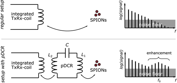
Figure 1. Working principle of the passive dual coil resonator (pDCR). Top: the SPIONs' signal is directly picked up by the integrated transmit/receive coil (TxRx). The induced signal in frequency space decreases with frequency and vanishes in the noise floor at higher frequencies. Bottom: the signal is picked up by the central pDCR coil L1 with high sensitivity and is coupled into the integrated TxRx-coil by the outer pDCR coil L2. The coils L1 and L2 are connected via a capacitor C enabling frequency-selective signal enhancement around the pDCR resonance frequency f0.
Download figure:
Standard image High-resolution imageNote that this is a simplified model, i.e. there will also be coupling between the particle magnetization and L2 as well as between L1 and the integrated Rx-chain. However, the impact of those can be regarded as minor compared to the above-mentioned signal pathway.
2.2. Mechanical design
We aimed to fulfill three main requirements with the mechanical realization of the pDCR: first, the used materials should not affect the MPI's imaging process; thus, electrically conductive and magnetic materials were unsuitable. Second, the pDCR needs to be easy to handle in a lab-environment and allow uncomplicated cleaning processes while withstanding disinfecting agents, e.g. after use for potential in vivo experiments. Third, the device should be fastly adaptable and cost-effective.
To fulfill these demands, we chose a combination of machined acrylic glass (PMMA) tubes as carriers for the inner and outer coil as well as 3D-printed alignment plates. The inner tube was designed to host the animal support. It is elongated towards the user end, which allows it to serve as mechanical fixation and reference with respect to the animal bed holder (Minerve SA, Esternay, France). The alignment plates ensure the concentric alignment of the coil carrier and allow fixation in the MPI's bore. Several holes placed in the alignment plates ensure air exchange between the inner and outer coil in the case of thermal heating. All connections use plastic screws, which allow easy maintenance and adaption of the device. A technical drawing, a 3D CAD model and a photograph of the pDCR in front of the scanner bore are shown in figure 2.
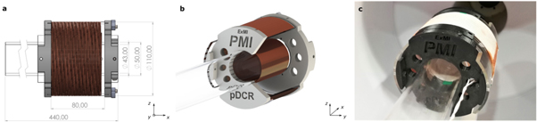
Figure 2. Technical drawing, 3D CAD model and photograph of the assembled pDCR: (a) technical drawing of the pDCR (side view) with the most relevant dimensions specified. (b) CAD design of the pDCR. A three quarter section view of the pDCR reveals the inner coil. (c) Photograph of the assembled pDCR in front of the preclinical MPI system's bore. The Litz wire cables that lead to the capacitor are visible in the front.
Download figure:
Standard image High-resolution image2.3. Specifications
Each of the solenoid coils is made of 31 turns that are continuously wound on the respective carrier cylinder. The diameter of the inner and outer carrier is 50 mm and 110 mm, respectively. Copper Litz wire (Rupalit V155, Rudolf Pack GmbH & Co. KG, Gummersbach, Germany) with a diameter of 1.5 mm (2300 × 0.02 mm) was used. The total inductance of both coils in series is Ltot = 210 μH at 700 kHz. The capacities C were varied to realize different resonance frequencies f0. The pDCR aims to enhance the SNR of frequency components, which usually vanish in the noise floor. This often happens at the right edge of the maximum of the integrated LNA's frequency response (approx. 400 kHz), which is the target region of the pDCR resonance frequency. Finally, the pDCR was tuned to {685, 710, 750, 800} kHz. In the following, each version will be called according to its specific resonance frequency in kHz.
Inserted into the scanner bore, the resonance frequency of the pDCR shifts due to interactions with hardware components as shielding components, focus field coils and the transmit/receive setup of the MPI system. The resonance frequencies outside and inside the scanner bore f0 out and f0 in, as well as the capacities C used for tuning can be taken from table 1.
Table 1. Specifications of pDCR Versions. The resonance frequency of the pDCR outside the MPI system  changes when the device is inserted into the scanner bore
  .
.
| Label |

|

| Capacitance C |
|---|---|---|---|
| pDCR-685 | 685 kHz | 585 kHz | 340 pF |
| pDCR-710 | 710 kHz | 620 kHz | 314 pF |
| pDCR-750 | 750 kHz | 660 kHz | 273 pF |
| pDCR-800 | 800 kHz | 710 kHz | 246 pF |
2.4. Receive chain characterization
In order to characterize the receive chain, the power transfer through the Rx-channel was determined. This was done for the regular Rx-channel only (bore diameter: 119 mm; TxRx-coil diameter: 156 mm), for each version of the pDCR inserted into the MPI bore, and for the dedicated rat-sized receive coil (bore diameter: 65 mm). The rat coil is a commercial product that comes along with an own matched receive chain.
To measure the power transfer, a small transmit coil was built that can be driven to the bore center with the help of the MPI robot. The coil is made of enameled copper wire that is wound three times on a 3D-printed cubic carrier with 7 mm edge length. The coil was connected to the output of a network analyzer and the output of the integrated LNA of the scanner's Rx-channel was connected to the input. The power transmission measurement was performed in the frequency range of 10 kHz to 2 MHz. The receive bandwidth of the scanner is 1.25 MHz.
The pDCR was positioned in the bore center by slowly pushing it further until the resonance peak intensity of the transmission function reached its maximum. The end position of the elongated inner pDCR coil carrier was marked at the animal bed rail to enable reproducible positioning of the pDCR.
2.5. System matrix acquisitions
System matrices were acquired to evaluate the performance of the pDCR with respect to SNR and as calibration for later measurement-based image reconstruction. All system matrix acquisitions and phantom measurements were performed with a 10 mg(Fe) ml−1 dilution of in-house developed SPIONs called C2 (Dadfar et al
2020). The size-isolated and almost monodisperse magnetic nanoparticles are obtained by co-precipitation. The mean core size and hydrodynamic diameter are 9–11 nm and 49 mm, respectively. C2 provides 2.3 times higher SNR per iron mass than Resovist (Bayer Pharma AG, Berlin, Germany) (Lawaczeck et al
1997) and a similar full width at half maximum (FWHM) of the point spread function (PSF). The volume of the reference sample for each acquired SM was 8 μl. The SMs are composed of 25 × 20 × 8 voxels (x, y, z) with a size of 1 × 1 × 1.5 mm3, resulting in a SM FOV of 25 × 20 × 12 mm3. The resolution in z-direction could be reduced, since the spatial resolution is evaluated in the x–y-plane. The maximum gradient strength was set to  = 2.5 T m−1 in z-direction. The drive field amplitudes in all three spatial directions were
  = 14 mT. The SMs were averaged 500 times. For background correction, the background is acquired intermittently during the SM acquisition. The mean SNR of the SM as computed by the Bruker software Paravision was used for SNR evaluation. It is defined for each frequency fj
as the mean signal across all SM voxels
= 14 mT. The SMs were averaged 500 times. For background correction, the background is acquired intermittently during the SM acquisition. The mean SNR of the SM as computed by the Bruker software Paravision was used for SNR evaluation. It is defined for each frequency fj
as the mean signal across all SM voxels  divided by the mean of the background signal
  , both after background correction (Franke et al
2016).
, both after background correction (Franke et al
2016).
For evaluation, the number of frequency components with an SNR above a certain threshold was analyzed. Cutting of all frequency components below a selected SNR threshold is a common approach that removes noisy frequency components from the SM to enhance image quality and accelerate the reconstruction process. The investigated cutoff values varied from 1.5 up to 10 in steps of 0.1. In addition, the frequency components of each acquired SM, which feature an SNR value above 2, were analyzed regarding their mixing orders.
Prior to image reconstruction, SM denoising was applied with a frequency domain filter based on a discrete cosine transform (Weber et al 2015). 'Soft' thresholding with the threshold value of 0.03 was used.
2.6. Phantom measurements
The resolution phantom is made out of PMMA. Bores with a diameter of 0.5 mm and a depth of 3 mm are arranged with increasing distance. The distance between the bores increases from 2 mm to 6 mm center-to-center, which corresponds with 1.5–5.5 mm edge-to-edge. All dimensions of the phantom can be taken from the technical drawing that is shown in figure 3. The bores were completely filled with a 10 mg(Fe)/ml dilution of C2 and sealed with epoxy resin. The tracer that is filled inside a bore will be called rod in the following.

Figure 3. Technical drawing of the resolution phantom (dimensions in mm). The phantom is made out of PMMA. It features bores with a diameter of 0.5 mm and a depth of 3 mm. The distance between the bores increases from 1.5 mm to 5.5 mm (edge-to-edge). The bores are filled with a 10 mg(Fe) ml−1 dilution of SPIONs (rod) and sealed with epoxy resin.
Download figure:
Standard image High-resolution imageThe resolution phantom was positioned in the center of the bore with the help of the robot. The orientation of the phantom can be taken from the coordinate system displayed in figure 3. For background correction, an empty measurement was taken after each phantom acquisition. Each image acquisition was performed with the same acquisition parameters (number of averages navg = 1000,  = 14 mT,
  = 2.5 T m−1) for all investigated setups.
For image reconstruction, the Kaczmarz algorithm with physical constraints enforcing positive and real values implemented in Python was used. The image reconstruction was performed on the full set of acquired data from all three receive channels. For each image reconstruction, the same parameters were set (number of iterations niter = 500, regularization parameter λ = 1e−5, SNR threshold = 2), except for the image reconstruction of the phantom acquired with the rat coil, where λ = 1e−7. The resulting total number of frequencies that were used for reconstruction depended on the individual SMs.
To evaluate the spatial resolution, the line profile through the two rods with a distance of 2.5 mm (edge-to-edge) is observed, since these can just be separated.
3. Results
3.1. Receive chain characterization
The measured power transfer functions are depicted in figure 4. At 25 kHz, the transmission functions show a dip that originates from the band-stop filter that is integrated in the scanner's receive chain. The band-stop functionality is not perturbed by the pDCR. The maximum gain between 300 kHz and 400 kHz is caused by the resonance of the integrated LNA.
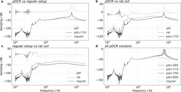
Figure 4. Absolute power transfer through the different investigated receive chains. The damping is measured in dB (voltage level): (a) MPI system's (Bruker Biospin MRI GmbH, Ettlingen, Germany) x-receive channel only (regular) and setup with inserted pDCR-710. (b) pDCR-710 setup and the dedicated rat coil setup (Bruker Biospin MRI GmbH). (c) Regular setup and the dedicated rat coil setup. A difference plot of the mentioned transfer functions is added to the respective figures. (d) The transfer functions of all pDCR versions with varying resonance frequency.
Download figure:
Standard image High-resolution imageIn figure 4(a), the transfer function of the regular Rx-chain and the pDCR-710 setup is shown together with a difference plot. The difference plot shows that both functions closely match up to approximately 200 kHz. Then, the resonance effect of the pDCR becomes visible and it peaks at the resonance frequency f0. The maximum gain at the peak compared to the regular Rx-chain is +43.5 dB (voltage level). At 1.25 MHz, which is the maximum receive bandwidth of the preclinical MPI system, the gain is still +6 dB.
Comparing the transfer function of the pDCR-710 to the dedicated rat coil setup (figure 4(b)), only the resonance peak of the pDCR-710 from 530 kHz up to 920 kHz rises up against the transfer function of the rat coil setup. At peak, the gain by the pDCR is +31.9 dB.
The rat coil setup provides an almost uniform gain between +11.4 dB and +14.4 dB for frequencies >100 kHz compared to the regular Rx-chain. This is shown in figure 4(c).
In figure 4(d), the transfer functions of all assembled pDCR versions are shown together with the transmission function of the regular setup. The transfer function of the different pDCR versions only vary near the resonance peak and converge departing from the resonance frequency. The amplitude at peak is almost uniform across the different coil inserts at approx. −1.7 dB.
3.2. System matrix acquisitions
The mean SNR of the system matrices in frequency space is shown in figure 5. Overall, the SNR plots mirror the frequency response of the respective receive chains. This is illustrated in figure 5, bottom right.
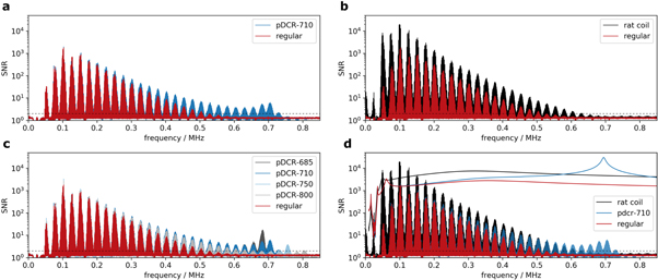
Figure 5. Mean SNR over all spatial positions of the system matrices acquired using the (a) pDCR-710 versus regular setup, (b) dedicated rat coil versus regular setup, (c) all pDCR versions versus regular setup, (d) rat coil, pDCR-710 and regular setup. The SNR threshold of 2 is highlighted by the dashed line. Figure (d) further illustrates that the SNR of the SM acquired using the pDCR is enhanced at the resonance. This is indicated by the depicted measured power transmission functions.
Download figure:
Standard image High-resolution imageComparing the mean SM SNR plots of the pDCR versions with the regular setup, the SNR gain achieved by inserting the pDCR increases up to the resonance frequency of the respective pDCR. Then, the SM SNR of each pDCR rapidly converges to the noise floor.
The mean SM SNR of the different setups at resonance can be taken from table 2. The SNR at resonance is maximum for the pDCR-685 and then decreases for increasing resonance frequency.
Table 2. Parameters for system matrix evaluation: SNR at pDCR resonance SNR(f0) (for the regular and the rat coil, the SNR at 685 kHz is shown). The max. frequency component with an SNR above 2  (SNR > 2). The number of frequency components after SNR cut-off nf.c.(SNR > 2). The max. mixing order after SNR cut-off
  (SNR > 2).
| Label | SNR(f0) |
 (SNR > 2) (SNR > 2) | nf.c.(SNR > 2) |
 (SNR > 2) (SNR > 2) |
|---|---|---|---|---|
| pDCR-685 | 17.2 | 711.4 kHz | 3742 | 29 |
| pDCR-710 | 6.4 | 732.8 kHz | 3792 | 30 |
| pDCR-750 | 3.9 | 763.5 kHz | 3207 | 30 |
| pDCR-800 | 2 | 806.3 kHz | 3132 | 32 |
| Regular | <2(685 kHz) | 507.7 kHz | 2458 | 21 |
| Rat | <2(685 kHz) | 632.5 kHz | 4736 | 25 |
The highest frequency component with an SNR > 2 of each investigated setup is listed in table 2. The value is lowest for the regular setup, followed by the rat coil and is max. for the pDCR SMs, where the value increases with f0.
The mean SM SNR for the different setups was analyzed with respect to the number of frequency components above the SNR thresholds between 1.5 and 10. The results are shown in figure 6(a) and in table 2 for the SNR threshold of 2. The dedicated rat coil setup performs best for all SNR thresholds. The SMs of all the examined pDCR setups provide an increased number of frequency components over the observed SNR range compared to the regular setup. Within the examined pDCR versions, the pDCR-710 performs best.

Figure 6. (a) Number of system matrix frequency components above a certain SNR threshold for the different receive chain setups (x-channel). (b) Abundance distribution of high mixing orders (20–32) in the acquired system matrices that exceed the SNR of 2 (x-channel).
Download figure:
Standard image High-resolution imageFigure 6(b) shows the abundance distribution of mixing orders in the acquired SMs. Only frequency components that exceed the SNR of 2 are considered. Since we are interested in the number of frequency components with high mixing order, the figure shows the frequency of mixing orders from 20 to 32. The maximum mixing order for each acquired system matrix is listed in table 2. The pDCR SMs contain the highest mixing orders compared to the regular and the rat coil setup.
The signal distributions of the acquired SMs at specifically selected frequency components are depicted in figure 7. The component with maximum SNR close to the respective resonance frequency was selected for each system matrix. For each SM frequency component, the z-slice with maximum signal intensity is depicted. The pixel intensities are normalized to the maximum signal intensity of the respective SM frequency component. The signal phases and amplitudes are rgba-color encoded as proposed in Heinen et al (2017).
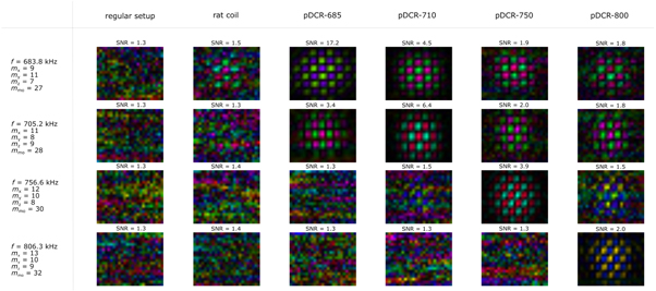
Figure 7. Spatial signal distributions of the acquired system matrices at specifically selected frequency components close to the resonance frequencies f0 of the pDCR versions. For each system matrix, the z-slice with highest signal intensity is shown. The signal intensities are normalized and the phases and amplitudes are rgba-color encoded. The mixing factors and the resulting mixing orders are shown below the respective selected frequencies on the left.
Download figure:
Standard image High-resolution imageThe SM of the regular setup (left column) does only show noise at the selected frequencies. The rat coil SM (second column) only provides the expected spatial pattern at 683.8 kHz, however, it is still very noisy. In contrast, the characteristic spatial intensity distribution of the SM measured with the pDCR-685 (third column) at 683.8 kHz is clearly visible with high mean SNR and is visible at 705.2 kHz as well. The other pDCR versions also provide the expected spatial signal distributions at their specific resonance frequencies. In general, the frequency range, where components with visible spatial patterns are located, increases with increasing pDCR-resonance frequency. However, the SNR at resonance of those setups decreases with increasing resonance frequency.
3.3. Phantom image reconstructions
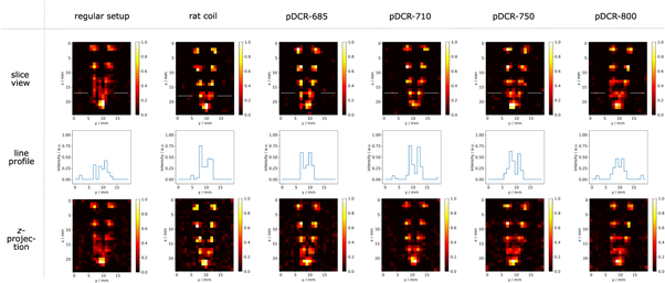
The reconstructed images of the resolution phantom are shown in figure 8. The upper row shows the slices in the x–y-plane, which feature the highest signal intensity of each 3D dataset. The line profiles (y-direction) that cross the two rods with 2.5 mm distance (edge-to-edge) are depicted in the middle row. The y-position of the line profile is indicated by two white lines in the respective slice view. It varies slightly due to positioning. The bottom row shows the projection along the z-axis of each 3D dataset. Each image is normalized to its maximum signal intensity.
Figure 8. Image reconstructions of the resolution phantom. Top row: slices in x–y-plane, which feature the maximum signal intensity of the respective image reconstruction. Middle row: respective line profiles (y-direction) through the rods with 2.5 mm distance (white lines). Bottom row: z-projection through the whole 3D dataset. Each image is normalized to its maximum signal intensity.
Download figure:
Standard image High-resolution image
Observing the phantom image acquired using the regular TxRx-coil, the rods with a distance of 3.5 mm can be distinguished well in the slice view as well as in the projection view. The rods with smaller distance cannot be identified clearly, the area around these rods is strongly blurred.
In the phantom image acquired using the dedicated rat coil, the rods with 2.5 mm distance can be distinguished well. This holds true for the slice as well as for the projection view. On the other hand, these two rods still appear slightly blurred. In the profile view, especially the right rod is poorly pronounced. Here, the signal intensity might be distributed into two bins. Further, the intensity between the rods drops only weakly.
Among all the pDCR setups, the pDCR-710 performs best regarding the spatial resolution. The rods with 2.5 mm distance can be distinguished very well, especially in the slice view, but also in the projection view. The line profile also shows that the rods are represented very sharply, with a steep dip in between the maxima.
Comparing the phantom image reconstruction from the acquisition using the regular setup with the sharpest image acquired using a pDCR (achieved with pDCR-710), the pDCR provides considerable spatial resolution enhancement. The rods with a distance of 2.5 mm can be clearly separated, which is not the case for the regular setup.
The phantom image quality obtained using the rat coil and the pDCR-710 appear similar at first glance. Focusing on the pair of rods with 2.5 mm distance, they can be distinguished slightly better in case of the pDCR-710, since the dip in between the rods is deeper and the right rod in the rat coil image is slightly blurred.
4. Discussion
Four different pDCR setups varying in resonance frequency have been evaluated and compared to the integrated receive chain and a dedicated rat coil insert in this study. For evaluation, the power transmission through the receive chain, the system matrix mean SNR at resonance, the number of frequency components of the SM above a certain SNR threshold, the mixing order of the SM frequency components with an SNR > 2 and the spatial resolution of phantom image reconstructions were analyzed.
Regarding safety of the receive electronics, overvoltage at the analog-to-digital converter (ADC) might be an issue. Measurements of the current in the pDCR have shown that the current is mainly flowing at the drive field frequency (approx. 40 mA amplitude at 14 mT drive field), thus overvoltage at the pDCR resonance can be excluded.
The power transfer function shows the frequency-dependent signal transfer through the receive chain and thus mirrors the frequency-dependent sensitivity of the respective channel. Analyzing the transfer functions depicted in figure 4, we could show that the pDCR provides frequency-selective sensitivity enhancement compared to the integrated receive chain. Compared to the dedicated rat coil, the pDCR provides increased sensitivity over a narrower frequency region (530–920 kHz for pDCR-710). However, there is still a considerable sensitivity gain of 31.9 dB at resonance.
Figure 4(d) further shows that the pDCR can be designed with different resonance frequencies without any considerable loss of sensitivity at resonance between 685 kHz and 800 kHz. The optimal pDCR resonance frequency with respect to image quality may depend on different parameters as tracer behavior (e.g. tracer volume of measured object, tracer distribution and concentration, SNR per iron mass), scanner properties and acquisition parameters that affect the SNR pattern in frequency space.
For potential future applications, it may be advantageous to use a tunable pDCR, where the resonance frequency can be easily tuned according to the planned MPI measurement. For instance, if the expected tracer concentration or amount is low, it will be more advantageous to use a lower resonance frequency and vice versa.
The mean SNR spectra (see figure 5) of the acquired SMs prove that the pDCR enhances the SNR at and nearby the resonance frequency. The mean SNR spectra qualitatively validate the frequency-dependent sensitivity curves of the receive chains (see figure 4), since the regions of SNR gain achieved by the pDCR correspond to the regions of sensitivity gain (see figure 5 bottom right).
The pDCR-800 provides the highest frequency component with an SNR > 2. However, it only features an SNR of 2. Between approx. 650 kHz and 800 kHz, all frequency components are below 2 and only some are slightly above the noise floor. An SNR threshold of min. 2 is usually applied during image reconstruction. Thus, these frequency components would be neglected and above 650 kHz, only some frequency components at resonance would be taken into account. The pDCR-750 shows a similar behavior between approx. 650 kHz and 720 kHz.
The number of frequency components that are considered during image reconstruction strongly affects the reconstruction quality. If the added information is not redundant, increasing the number of frequency components reduces the condition number of the linear equation system, which increases the stability of the reconstruction result against noisy or corrupt frequency components.
Figure 6(a) proves that the pDCR is able to increase the number of frequency components above a certain SNR threshold compared to the regular setup. All pDCR versions outperform the regular setup. Although the maximum frequency component of the rat coil SM with an SNR value above 2 is at 632.5 kHz, this setup provides the most frequency components above the considered thresholds. This enhancement mainly stems from the intermediate components in between the harmonics.
The spatial patterns of specifically selected SM frequency components (see figure 7) validate the SNR gain of the pDCR compared to the regular setup and the rat coil at their specific resonance frequencies. The expected spatial signal distributions can be recognized very clearly in case of all the different pDCR versions at their specific resonance frequencies. This proves that the lifted frequency components include spatial information. The expected number of extrema in the spatial patterns cannot be observed, which is most probably due to the fact that the drive field FOV exceeds the system matrix FOV in y-direction. Additionally, the signal at the edges of the FOV is low and thus, some maxima are not visible. Besides that, relaxation effects and aliasing effects due to the sample size and SM grid may play a role.
Image reconstructions of a resolution phantom (see figure 3) were analyzed with respect to spatial resolution (see figure 8). Since the edge-to-edge distance of the rods that could be clearly separated is 2.5 mm, the achieved spatial resolution is below 2.5 mm. The distance between the maxima in the spatial patterns of the SMs indicate that the achievable spatial resolution with the pDCR is higher than the actually achieved image resolution.
The spatial resolution could potentially be further enhanced with using a smaller SM reference sample, reducing voxel size or using different SPIONs. A direct integration of a mechanical reference point inside the bore and mechanical fixation of the capacitor outside the bore would increase f0 stability and probably further improve the image quality. Heating of the pDCR was evaluated with an infrared camera. Although no heating was found using the measurement routine, slight temperature shifts cannot be excluded and could be further investigated. However, the gain of stability needs to be weighed against the effort and costs of a cooling strategy.
The reconstruction parameters were selected based on the subjective impression of the highest spatial resolution, while minimizing the overall noise in the image. To ensure a fair comparison, the reconstruction parameters were kept constant for all image reconstructions, except for the reconstruction of the rat coil image. Here, less regularization was needed to achieve the best trade-off between spatial resolution and noise, probably due to the increased number of frequency components above the selected SNR threshold 2 and the higher mean SNR over the used frequency components.
Comparing the four different pDCR versions, one can conclude that the pDCR-710 performs best regarding spatial resolution. These results correspond to the performance of the different setups regarding the SM SNR and the number of frequency components above the SNR threshold of 2. While the SNR at resonance is higher for the pDCR-685, the pDCR-710 provides slightly more frequency components above the SNR of 2 and the enhanced frequency components of the pDCR-710 are at higher frequencies, which are related to higher mixing orders.
The images acquired with the regular TxRx-coil provide the worst spatial resolution among all investigated setups. This result matches the findings from the SM SNR and the mixing orders of the respective SM frequency components. One can conclude that the pDCR demonstrates spatial resolution enhancement compared to the regular setup.
The images acquired using the dedicated rat coil provide good spatial resolution but do not outperform the images acquired with the pDCR-710. This is remarkable considering the great overhead of the dedicated rat coil coming along with high costs and installation effort compared to the simplicity and cost-efficiency of the pDCR. The rat coil was not able to outperform the pDCR, although the SM acquired with the rat coil provides more frequency components above the SNR threshold of 2. This is most likely due to the fact that the pDCR-710 provides many frequency components with high mixing orders from 26 to 30 resulting from the pDCR resonance, while the maximum mixing order provided by the rat coil is 25.
5. Conclusion
In this manuscript, we present a novel concept for frequency-selective signal enhancement enabled by a cost-effective and purely passive coil insert. The pDCR fits the bore of a preclinical MPI system and comes along without any additional receive equipment. In order to lift frequency components featuring high mixing orders out of the noise, the pDCR was tuned to resonance frequencies between 685 kHz and 800 kHz. We have shown that using the pDCR increases the mean system matrix SNR at and nearby the resonance frequency. The pDCR system matrices feature higher mixing orders when considering frequency components with SNR > 2, compared to the integrated transmit/receive coil only and a dedicated rat coil with separate receive unit. Image reconstructions of a resolution phantom have shown that the pDCR is able to increase the image quality in terms of spatial resolution.
Acknowledgments
This work was supported in part by the German Research Foundation (DFG, project number 441892463).