
Abstract
The empirical conversion of the treatment planning x-ray computed tomography (CT) image to ion stopping power relative to water causes dose calculation inaccuracies in ion beam therapy. A patient-specific calibration of the CT image is enabled by the combination of an ion radiography (iRad) with the forward-projection of the empirically converted CT image along the estimated ion trajectories. This work investigated the patient-specific CT calibration for list-mode and integration-mode detector configurations, with reference to a ground truth ion CT (iCT) image. Analytical simulations of idealized carbon ion and proton trajectories in a numerical anthropomorphic phantom and realistic Monte Carlo simulations of proton, helium and carbon ion pencil beam scanning in a clinical CT image of a head-and-neck patient were considered. Controlled inaccuracy and noise levels were applied to the calibration curve and to the iRad, respectively. The impact of the selection of slices and angles of the iRads, as well as the choice of the optimization algorithm, were investigated. Accurate and robust CT calibration was obtained in analytical simulations of straight carbon ion trajectories. Analytical simulations of non-straight proton trajectories due to scattering suggested limitations for integration-mode but not for list-mode. To make the most of integration-mode, a dedicated objective function was proposed, demonstrating the desired accuracy for sufficiently high proton statistics in analytical simulations. In clinical data the inconsistencies between the iRad and the forward-projection of the ground truth iCT image were in the same order of magnitude as the applied inaccuracies (up to 5%). The accuracy of the CT calibration were within 2%–5% for integration-mode and 1%–3% for list-mode. The feasibility of successful patient-specific CT calibration depends on detector technologies and is primarily limited by these above mentioned inconsistencies that slightly penalize protons over helium and carbon ions due to larger scattering and beam spot size.
Export citation and abstract BibTeX RIS

Original content from this work may be used under the terms of the Creative Commons Attribution 3.0 license. Any further distribution of this work must maintain attribution to the author(s) and the title of the work, journal citation and DOI.
1. Introduction
Although physical and radiobiological properties of ion beams foster an improved targeting in radiation therapy when compared to photon beams, the superior dose conformality offered by scanned ion beams comes at the expense of enhanced sensitivity to inaccuracies (Durante and Loeffler 2010). Among others, inaccuracies are intrinsically related to the current clinical treatment planning, due to uncertainties in the knowledge of the ion stopping power properties of different tissues (Schneider and Pedroni 1995, Schaffner and Pedroni 1998). Treatment planning is typically performed on x-ray computed tomography (CT) images, expressed as relative photon linear attenuation coefficients (Hounsfield Unit, HU). In order to match the specific physical and radiological properties of the therapeutic radiation, the CT image undergoes an empirical calibration, usually relying on a plastic phantom provided with tissue equivalent inserts. In ion beam therapy, the CT image is converted to ion stopping power relative to water (RSP) (Schneider et al 2000), referred to as rspCT image, as this ratio is needed by analytical dose calculation algorithms to scale the well-known depth dose distribution in water to any arbitrary tissue (Hong et al 1996, Schaffner et al 1999). A stoichiometric calibration is usually adopted, based on a parameterization of the HU in elemental composition and mass density (Schneider et al 1996). Information about different elemental compositions can be also derived from dual-energy CT image (Bourque et al 2014). Although the stoichiometric calibration overcomes the approximation of the elemental composition for biological tissue with tissue equivalent inserts, tissue-specific and patient-specific variations of elemental compositions are responsible for up to 3% of remaining inaccuracies in the calibration curve (Jiang et al 2007, Yang et al 2012), thus translating into inaccuracies in range estimation up to several millimeters (Rietzel et al 2007, Paganetti 2012).
Ion imaging has the potential of directly measuring the tissue stopping power properties to overcome intrinsic inaccuracies in treatment planning (Parodi 2014). The residual energy of energetic ions after traversing the object of interest is measured relying on a total absorption detector and then calibrated to the equivalent ion beam range in water or water equivalent thickness (WET). The WET matches the integral RSP along the traversed object of interest. When the ions are individually tracked, each ion carries a WET. This 'list-mode' detector configuration is typically synchronized with a tracking system before and after the object of interest, thus enabling the estimation of the ion trajectories (Schulte et al 2008). Scanned ion beams offer the possibility to simplify the detector configuration by removing the tracking system and synchronizing the total absorption detector with the pencil beam delivery system. With this 'integration-mode' detector configuration, the WET is carried by the ensemble of ions in the pencil beam. The ion trajectories are statistically distributed according to the beam spot size (BSS) and the multiple Coulomb scattering (MCS) model. Although ions are not individually tracked, information about WET inhomogeneity can be retrieved by discretizing the total absorption detector (Rinaldi et al 2013), thus detecting range mixing effects in the discrete energy loss signal. For each pencil beam, a WET histogram expressing the weight of each WET component can be obtained by means of a linear decomposition of the signal (Meyer et al 2017). Accounting for the estimation of the ion trajectories provided by different detector configurations, the measurements covering the object of interest at a certain angle are typically organized in an ion radiography, or iRad. The combination of an iRad with the rspCT image enables a patient-specific calibration of the CT image to RSP (Schneider et al 2005). This calibration relies on the forward-projection of the rspCT image along an estimation of the ion trajectory (yielding the water equivalent Digitally Reconstructed Radiography, weDRR). The patient-specific calibration of the CT image to RSP can be implemented as a linear minimization if prior segmentation of the rspCT image is applied. Alternatively, an optimization algorithm embedding forward-projection and segmentation of the iteratively adjusted rspCT image can be adopted. Despite the computational advantage of a linear minimization (Collins-Fekete et al 2017, Zhang et al 2018, Krah et al 2019), the adoption of a non-linear optimization algorithm enables to overcome the limitation of the prior segmentation and the forward-projection of the rspCT image (Schneider et al 2005, Doolan et al 2015). Depending on the detector configuration, the trajectory is either estimated for each ion (list-mode) (Collins-Fekete et al 2017) or assumed to be a straight line for each pencil beam (integration-mode) (Doolan et al 2015, Zhang et al 2018, Krah et al 2019).
In this work, the patient-specific calibration of the CT image based on iRads is extensively investigated in analytical simulations of idealized carbon ion and proton trajectories in a numerical anthropomorphic phantom (Göppel et al 2017). The role of the MCS as well as the BSS in both ideal list-mode and integration-mode detector configurations is assessed. Two different non-linear optimization algorithms are compared to linear minimization. The first one is adopted from a previous work targeted to integration-mode detectors (Doolan et al 2015) and the second one is chosen for its flexibility, as required by CT calibration when no assumption about the inaccuracy model of the calibration curve is made. To make the most of integration-mode detector configuration, a dedicated objective function based on the entire WET histogram is proposed. Relying on the investigation in analytical simulations, the patient-specific calibration of the CT image based on iRads for different detector configurations in proton, helium and carbon ion pencil beam scanning is investigated in Monte Carlo simulations at clinically acceptable imaging dose in a clinical CT image of a head-and-neck patient.
2. Materials and methods
2.1. Analytical simulations in numerical anthropomorphic phantom
The photon linear attenuation coefficients of a numerical anthropomorphic phantom (Segars et al
2002) were linearly transformed to HUs. Subsequently, the generated CT image was converted to the ground truth ion CT (iCT) image relying on a monotonic calibration curve, referred to as true calibration curve. The calibration curve was made of 13 points, one for each linear attenuation coefficient of the numerical anthropomorphic phantom, according to a histogram-driven point selection of the calibration curve. Each point was associated with a point weight equal to the corresponding abundance in the image. The size of the images was  voxels. The pixel size was
  cm3. An inaccurate calibration curve was created by applying controlled inaccuracies Δ to the points of the true calibration curve. The inaccurate calibration curve was then used to generate the rspCT image. The inaccuracies were generated under the constraint of monotonically increasing calibration curve, randomly sampled from a uniform distribution over realistic intervals.
The idealized carbon ion and proton trajectories outline the best and the worst cases of MCS, respectively. The idealized carbon ion trajectories were traced as straight lines along the pencil beam direction to simplify the negligible MCS and smaller BSS compared to protons. Therefore, no distinction between list-mode and integration-mode detector configurations was enabled. The idealized proton trajectories were simulated relying on a recently proposed analytical framework for both list-mode and integration-mode detector configurations in proton pencil beam scanning (Gianoli et al 2019). The proton trajectories were traced within the statistical distribution of the BSS and MCS model, neglecting energy straggling and nuclear interactions. The physical parameters of the analytical simulations were summarized in table 1. The iRad was simulated as forward-projection of the ground truth iCT image along the simulated trajectories. The iRad for list-mode corresponded to the WET for each ion of the pencil beam. In contrast, a WET histogram for each pencil beam was obtained for integration-mode, thus referred to as integration-mode hist. The WET histogram enabled the computation of a weighted mean WET (WET components weighted by the occurrences and averaged) and a mode WET (WET component with the maximum occurrence), thus referring to integration-mode mean and mode, respectively.
Table 1. Physical parameters of the analytical simulations of iRads for idealized proton trajectories.
| Idealized protons | |
|---|---|
| Proton pencil beam energy | 280 MeV |
| Number of protons per pencil beam (proton statistics) | 100, 75, 50, 25, 10, 5 |
| Standard deviation of the BSS (σBSS) | 0.0 cm (i.e. ideal pencil beam), 0.3 cm |
For the analytical simulations of idealized carbon ions, the weDRR was based on the straight lines coinciding with the simulated carbon ion trajectories. For the analytical simulations of idealized protons, the weDRR for list-mode was based on proton trajectories estimated using the Most Likely Path (MLP) algorithm (Schulte et al 2008). For integration-mode mean and mode, the estimated proton trajectories were traced straight along the pencil beam direction. Conversely, for integration-mode hist the proton trajectories were estimated according to a random sampling of the statistical distribution within BSS and MCS model along the pencil beam direction. The number of these samples, or proton statistics for the weDRR, was set equal to 100 protons per pencil beam. The weDRR was calculated as the forward-projection of the rspCT image along the estimated trajectories. For integration-mode hist, the forward-projection of the rspCT image generated a WET histogram for each pencil beam, similar to the corresponding iRad.
2.2. Monte Carlo simulations in clinical data
A clinical CT image of a head-and-neck patient from the Department of Radiation Oncology of the university hospital of the LMU Munich undergoing intensity modulated photon therapy treatment was considered. The CT image was converted to the ground truth iCT image relying on a calibration curve defined by 11 points, similar to the one used at the Heidelberg Ion Beam Therapy Center for treatment planing of head-and-neck patients. This calibration curve was assumed as true calibration curve. The size of the CT image was  voxels. The pixel size was
  mm3. The iRads for proton, helium and carbon ion were simulated in FLUKA (Ferrari et al
2005, Böhlen et al
2014) (public release version 2011.2c.6 using HADROTHE defaults without explicit delta-ray production), relying on a customized simulation framework (Meyer et al
2019) provided with phase space files of the Heidelberg Ion Beam Therapy Center (Tessonnier et al
2016). The weDRRs for proton, helium and carbon ions were based on trajectories estimated according to the cubic spline approximation of the MLP algorithm (Fekete et al
2015). The ion statistics for the weDRR, as required for the objective function dedicated to integration-mode hist, was set equal to the ion statistics of the iRad. The physical parameters summarized in table 2 resulted in a comparable physical dose for proton, helium and carbon ion iRads (0.01 mGy for low ion statistics and 0.26 mGy for high ion statistics).
mm3. The iRads for proton, helium and carbon ion were simulated in FLUKA (Ferrari et al
2005, Böhlen et al
2014) (public release version 2011.2c.6 using HADROTHE defaults without explicit delta-ray production), relying on a customized simulation framework (Meyer et al
2019) provided with phase space files of the Heidelberg Ion Beam Therapy Center (Tessonnier et al
2016). The weDRRs for proton, helium and carbon ions were based on trajectories estimated according to the cubic spline approximation of the MLP algorithm (Fekete et al
2015). The ion statistics for the weDRR, as required for the objective function dedicated to integration-mode hist, was set equal to the ion statistics of the iRad. The physical parameters summarized in table 2 resulted in a comparable physical dose for proton, helium and carbon ion iRads (0.01 mGy for low ion statistics and 0.26 mGy for high ion statistics).
Table 2. Physical parameters of the Monte Carlo simulations of iRads for proton, helium and carbon ion pencil beam scanning.
| Protons | Helium ion | Carbon ion | |
|---|---|---|---|
| Nominal pencil beam energy | 199.44 MeV | 199.03 MeV/u | 385.18 MeV/u |
| Number of ions per pencil beam (ion statistics) | 400 (low), 10 000 (high) | 100 (low), 2500 (high) | 20 (low), 500 (high) |
| Full width at half maximum of the BSS | |||
| (FWHMBSS) a | 8.5 mm | 5.1 mm | 3.5 mm |
a In air at the isocenter (Meyer et al 2019).
2.3. Patient-specific CT calibration based on iRads
The patient-specific CT calibration was implemented as an optimization algorithm that estimated the inaccuracies Δ to adjust the weDRR based on the iRad. Expressing the weDRR as the forward-projection (matrix-vector product) of the rspCT image (column vector, function of Δ) along the estimated trajectory (column vector in the matrix A, for all the trajectories),  , the optimization algorithm searches for the inaccuracies Δ as
N being the dimension of the weDRR and the iRad.
Accordingly, the optimization algorithm is expected to adjust the inaccuracies of the calibration curve towards the true calibration curves. The forward-projection and the segmentation of the iteratively adjusted rspCT image were embedded in the optimization algorithm. The objective function of the optimization algorithm was the root mean square error (RMSE) between the iRad and the weDRR. This objective function was expressed in voxels for list-mode as well as for integration-mode mean and mode. For integration-mode hist, the dedicated objective function was expressed as normalized WET occurrences (probability) for each pencil beam.
Five different seeds were selected to initialize the random number generator in order to obtain reproducible inaccuracies of the inaccurate calibration curve. The accuracy of the CT calibration was quantified as mean absolute relative error (MRE) between the points of the true and the optimized calibration curves. Median and interquartile range (iqr) MRE among the different random seeds were quantified. Successful CT calibration was defined as MRE below 1%.
2.4. Investigation in numerical anthropomorphic phantom
Relying on idealized carbon ion trajectories, two different non-linear optimization algorithms implemented in MATLAB (Matlab, MathWorks, Natick, MA, USA), namely Nelder–Mead (Lagarias et al 1998) and particle swarm (Kennedy 1995), were compared. In addition, linear minimization relying on the least-squares solver implemented in MATLAB was considered. The angles of the iRads was 0° (frontal iRad), 45°, 90° (lateral iRad) and 135°. The impact of the number of iRads at different angles and the number of slices for each iRad were investigated. In addition to the histogram-driven point selection of the calibration curve, an equally-spaced point selection within the minimum and the maximum of the linear attenuation coefficients was considered. The controlled inaccuracies Δ were applied according to both additive (RSP + Δ) and multiplicative (RSP ×(Δ + 1)) inaccuracy models in combination with histogram-driven and equally-spaced point selection of the calibration curve. To investigate the effect of an increase in inaccuracy level, the inaccuracies were applied within an interval spanning from ± 0.05 to ± 0.30 at additive steps of +0.05. The inaccuracies were applied to a progressively increasing number of points of the calibration curve (from one to all the 13 points of the calibration curve), according to both increasing and decreasing point weights. The effect of an increase in noise level on the iRads was also assessed. Either the experimental or the statistical nature of the noise was considered. Relying on idealized carbon ion trajectories, nine multiplicative noise levels simulating experimental noise were investigated. The variance spanned from 10–4 to 104 mm2, logarithmically spaced by 101 mm2. Relying on idealized proton trajectories, the effect of the statistical noise was assessed by decreasing proton statistics. Moreover, list-mode, integration-mode hist and integration-mode mean and mode were compared.
An overview of the investigation in numerical anthropomorphic phantom is reported in figure 1.
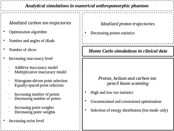
Figure 1. Overview of the investigation in numerical anthropomorphic phantom (dashed lines) and clinical data (continuous line).
Download figure:
Standard image High-resolution image2.5. Investigation in clinical data
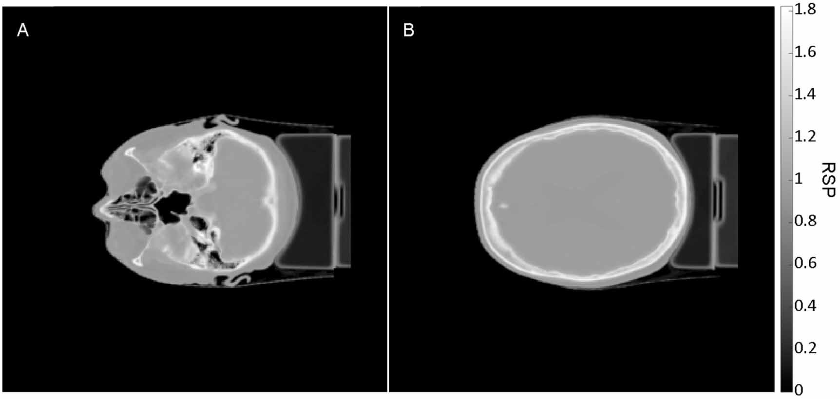
Inaccuracies were applied according to multiplicative inaccuracy models. The particle swarm was selected as optimization algorithm. The standard deviation of the WET for the ions of the pencil beam was calculated. In list-mode detector configuration, the ion trajectories were also selected based on 1, 2 and 3 times this standard deviation. The pencil beam scanning enabled the implementation of a data-driven, instead of the originally proposed model-driven, sigma cut (Schulte et al 2008). The lateral and the frontal iRads, as well as one slice crossing the nasal air cavity (nasal cavity slice) and one slice crossing the brain (brain slice) were selected (figure 2). For this selection, the normalized root mean square error (NRMSE) between the iRad and the weDRR of the ground truth iCT image, normalized by the latter, was quantified. The Wilcoxon signed rank test (5% significance level) was applied to support the statistical interpretation of results.

Figure 2. Nasal cavity slice and brain slice of the ground truth iCT image in clinical data.
Download figure:
Standard image High-resolution imageAn overview of the investigation in clinical data is reported in figure 1.
3. Results
3.1. Analytical simulations of idealized carbon ion trajectories in numerical anthropomorphic phantom
With an inaccuracy level within ± 0.05, the linear minimization resulted in median MRE equal to 3.30 × 10⁻⁹% and iqr MRE equal to 0.70% for the multiplicative inaccuracy model. The corresponding results for the additive inaccuracy model were 1.53% and 0.51%, respectively. With the same inaccuracy level, the Nelder–Mead algorithm demonstrated different results depending on additive or multiplicative inaccuracy models, reaching median and iqr MRE in the order of 10−11% for the multiplicative inaccuracy model but unstable results among the different random seeds for the additive inaccuracy model, with median MRE equal to 1.53 × 10⁻²% and iqr MRE equal to 8.47 × 10⁻²%. In contrast, the particle swarm algorithm reached instead median and iqr MRE in the order of 10−9% for both additive and multiplicative inaccuracy models. Relying on the particle swarm algorithm, the number of iRads at different angles and the number of slices demonstrated to have no impact, given that the iRad included all the points of the calibration curve. A CT calibration based on points that are not included in the iRads generated suboptimal results, as demonstrated by the equally-spaced point selection (median MRE of 2.09% and iqr MRE of 0.43%) or, although successful, the selection of slices that do not contain all the 13 points of the calibration curve (table 3). The effect of applying inaccuracies to a progressively increasing number of points of the calibration curve, according to both increasing and decreasing point weights, was negligible, with median MRE less than 10–8%. Selecting all possible combinations of number of iRads at different angles, the median and iqr MRE remained in the order of 10–9%–10−10%. Selecting two slices of the lateral iRad (figure 3), an increase in the inaccuracy level did not affect the CT calibration (figure 4). Instead, the increase in noise level (with an inaccuracy level within ± 0.05) severely affected the CT calibration, showing successful results only for small variance, equal to or less than 0.1 mm2 (figure 4).
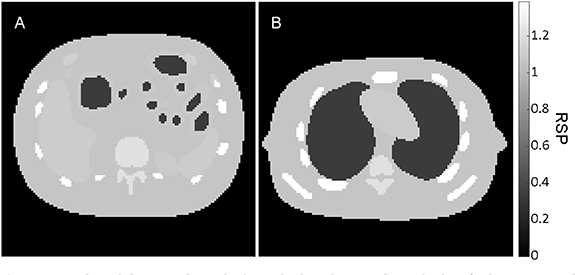
Figure 3. The abdomen slice {16} and the thorax slice {76} of the numerical anthropomorphic phantom.
Download figure:
Standard image High-resolution image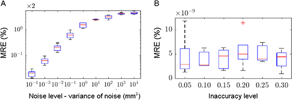
Figure 4. Median MRE (red line) and iqr MRE (blue box) for increasing noise (A) and inaccuracy (B) levels.
Download figure:
Standard image High-resolution imageTable 3. Selection of slices and the corresponding number of points of the calibration curve included in the iRad. Slices {16,76}, corresponding to abdomen and thorax respectively, contain all the 13 points of the calibration curve.
| Selected slices | {15,75} | {16,76} | {17, 77} |
| Number of points included in the iRad | 12 | 13 | 12 |
| Median MRE (iqr MRE) (%) | 3.1 × 10⁻¹ (1.1 × 10⁻¹) | 2.8 × 10⁻⁹ (4.2 × 10⁻⁹) | 3.8 × 10⁻¹ (8.6 × 10⁻²) |
3.2. Analytical simulations of idealized proton trajectories in numerical anthropomorphic phantom
Selecting two slices of the frontal iRad (figure 3), list-mode and integration-mode hist performed differently under reduction of proton statistics with an inaccuracy level within ± 0.05. Whereas list-mode yielded stable results (median MRE 0.12%, iqr MRE 1.33 × 10⁻⁴%) for all considered proton statistics, integration-mode hist revealed generally larger MRE and successful CT calibration for proton statistics down to five protons per pencil beam and (figure 5). Integration-mode mean and mode resulted in unsuccessful CT calibration. For 100 protons per pencil beam, the median MREs were 2.12% and 1.84%, respectively (the iqr MREs were 1.46 × 10⁻¹% and 1.59 × 10⁻¹%, respectively). The BSS caused unsuccessful CT calibration for integration-mode, whereas the accuracy for list-mode was better than 1% down to proton statistics equal to five protons per pencil beam (figure 5).

Figure 5. Median MRE (black line) and iqr MRE (colored box) for list-mode and integration-mode hist for σBSS equal to 0.0 cm (A) and 0.3 cm (B).
Download figure:
Standard image High-resolution image3.3. Monte Carlo simulations in clinical data
The optimization algorithm successfully converges in both detector configurations. List-mode enabled an improved accuracy of the CT calibration compared to inaccurate calibration curve (figure 6), but the accuracy was not always improved to be better than 1% as defined as successful calibration. Integration-mode gave worse results than simply relying on the inaccurate calibration curve (figure 7). The inaccuracies remained above 1% with an inaccuracy level within ± 0.05, thus determining an unsuccessful CT calibration. The NRMSE between the iRad and the weDRR of the ground truth iCT image expressed inconsistencies that explained the unsuccessful CT calibration (table 4). These inconsistencies reached about 9% for integration-mode mean and mode in proton pencil beam scanning and were hardly reduced below 1% for list-mode detector configuration in carbon ion pencil beam scanning. Larger NRMSE was quantified for integration-mode hist due to the normalization by smaller WET occurrences. These inconsistencies enabled a fluctuation of the optimized calibration curve in the order of the inaccuracies, thus preventing successful CT calibration. In general, integration-mode mean and mode performed worse than integration-mode hist. The latter remained worse than list-mode. Helium and carbon ions demonstrated slightly better accuracy than protons. The high ion statistics did not significantly benefit the CT calibration compared to low ion statistics. The statistical test applied to proton pencil beam scanning showed that there were no significant differences between low and high ion statistics. Statistically meaningful differences were instead observed in high ion statistics between protons and helium ions, as well as between protons and carbon ions.

Figure 6. Inaccurate and optimized calibration curves for list-mode detector configuration in proton pencil beam scanning at low ion statistics for nasal cavity slice (A) and brain slice (B) and for selected angles of the iRad and for inaccuracy level within ± 0.05.
Download figure:
Standard image High-resolution image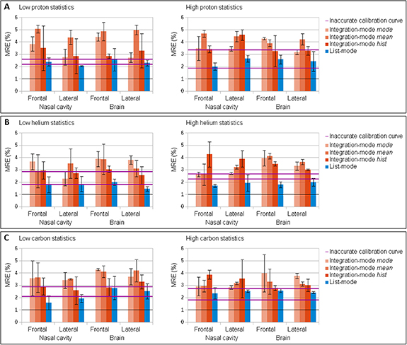
Figure 7. Median MRE (bar) and iqr MRE (error bar) for different detector configurations in proton (A), helium (B) and carbon (C) ion pencil beam scanning at low (left) and high (right) ion statistics for selected slices and angles of the iRad and for inaccuracy level within ± 0.05. The iqr MRE for the inaccurate calibration curve is traced by the two pink bold horizontal lines (25th and 75th percentiles). The MRE equal to 1%, as defined for successful CT calibration, is traced by a black horizontal line.
Download figure:
Standard image High-resolution image
Table 4. NRMSE (expressed in %) between the iRad and the weDRR of the ground truth iCT image, for different detector configurations in proton, helium and carbon ion pencil beam scanning at low and high ion statistics, for selected slices and angles of the iRad.
| Selected slices | Nasal cavity | Brain | |||
|---|---|---|---|---|---|
| Selected angle | Frontal iRad | Lateral iRad | Frontal iRad | Lateral iRad | |
| Low proton statistics | Integration-mode mode | 4.09 | 4.29 | 2.50 | 2.56 |
| Integration-mode mean | 4.79 | 8.93 | 4.23 | 8.18 | |
| Integration-mode hist | 13.16 | 8.91 | 18.74 | 4.89 | |
| List-mode | 2.12 | 2.54 | 1.44 | 2.01 | |
| High proton statistics | Integration-mode mode | 3.36 | 5.51 | 2.69 | 3.41 |
| Integration-mode mean | 5.38 | 9.50 | 4.24 | 7.96 | |
| Integration-mode hist | 4.74 | 13.33 | 11.58 | 30.27 | |
| List-mode | 2.13 | 2.64 | 1.48 | 2.06 | |
| Low helium statistics | Integration-mode mode | 2.61 | 2.99 | 1.52 | 3.67 |
| Integration-mode mean | 2.30 | 3.60 | 1.55 | 2.81 | |
| Integration-mode hist | 24.36 | 17.90 | 35.17 | 24.66 | |
| List-mode | 1.24 | 1.39 | 0.87 | 1.06 | |
| High helium statistics | Integration-mode mode | 3.46 | 3.95 | 3.89 | 2.48 |
| Integration-mode mean | 2.49 | 4.51 | 1.67 | 3.29 | |
| Integration-mode hist | 3.29 | 13.42 | 12.72 | 25.89 | |
| List-mode | 1.50 | 1.85 | 1.16 | 1.49 | |
| Low carbon statistics | Integration-mode mode | 2.59 | 2.59 | 2.23 | 2.07 |
| Integration-mode mean | 2.36 | 2.77 | 1.69 | 2.57 | |
| Integration-mode hist | 53.81 | 64.09 | 50.44 | ||
| List-mode | 0.95 | 0.96 | 0.77 | 0.80 | |
| High carbon statistics | Integration-mode mode | 2.36 | 3.13 | 1.77 | 2.49 |
| Integration-mode mean | 1.90 | 3.73 | 1.62 | 2.51 | |
| Integration-mode hist | 4.59 | 15.37 | 7.18 | 14.40 | |
| List-mode | 1.36 | 1.80 | 1.15 | 1.53 | |
To improve the accuracy of the CT calibration the constraint of monotonically increasing calibration curve was embedded in the optimization algorithm (appendix-table A1). Significant differences between constrained and unconstrained optimization, although small, were found in low proton statistics. The selection of multiple slices (appendix-table A2) and multiple angles (appendix-table A3) did not decisively improve results. Even the results for the lateral iRad resulted comparable to the results for the frontal iRad. The choice of the lateral iRad over the frontal one was supported by the separation of the treatment couch and the supporting pillow from the patient. Statistically meaningful differences between single angle and multiple angles as well as single slice and multiple slices were detected in low proton statistics when considering the highly inhomogeneous nasal cavity slice. For this slice, the lateral iRad statistically differed from the frontal iRad. The statistical test applied to high proton statistics showed that there were no significant differences between selections based on 1, 2 and 3 times the standard deviation of the ion energy (appendix-table A4).
4. Discussions
In this study, a patient-specific CT calibration based on iRad was investigated in a CT image of a head-and-neck patient, at clinically acceptable imaging doses, for both list-mode and integration-mode detector configurations. Proton, helium and carbon ion pencil beam scanning, with realistic energy compatible to current accelerator and detector technologies, were considered.
The selection of slices and angles of the iRads, as well as the choice of the optimization algorithm, was guided by an extensive investigation in analytical simulations in a numerical anthropomorphic phantom. In particular, the iRad should include all the points of the calibration curve matching the HUs of the CT image. Hence, the calibration curve should be defined as a function of the tissue linear attenuation coefficients or HUs of the CT image. Once this condition is met, a single iRad could be sufficient for the patient-specific CT calibration. To further investigate in this direction, a selection of the points of the calibration curve guided by their relevance in treatment planning (i.e. dose calculation inaccuracies) is currently under consideration. When comparing different optimization algorithms, better performance was obtained with the particle swarm algorithm independently of the inaccuracy models. Particularly, the multiplicative model can add more inaccuracies to RSP values larger than one and less inaccuracies to RSP values smaller than one. In other words, the multiplicative inaccuracy model shortens the axes of the multidimensional variable space corresponding to the points of the calibration curve from air to water (with smaller inaccuracies) and stretches those from water on (with larger inaccuracies). The update of the simplex of the Nelder–Mead algorithm seems favored by these shortening and stretching of the axes (appendix). This was likely the cause of the better performance with respect to the additive inaccuracy model. With the particle swarm algorithm, the motion of the particles is always consistent to the axes of the multidimensional variable space, either with additive or relative inaccuracy models. However, since the inaccuracy model in reality is unknown, an optimization algorithm sufficiently insensitive to the inaccuracy model, as demonstrated by the particle swarm, should be chosen.
The robustness against controlled inaccuracy levels of the calibration curve observed in analytical simulations of idealized carbon ion trajectories put forward the CT calibration feasibility based on less accurate in-room cone beam CT systems or even non-ionizing magnetic resonance imaging (Dowling et al 2012). However, in clinical data and in analytical simulations of idealized proton trajectories the CT calibration, although robust against high inaccuracy level (within ± 0.30), did not succeed at realistic inaccuracy level (within ± 0.05) because the inconsistencies between the iRad and the weDRR of the ground truth iCT image were in the same order of magnitude as the applied inaccuracies. In analytical simulation of idealized carbon ion trajectories, these inconsistencies were not present by construction.
These inconsistencies are differently present in list-mode and integration-mode detector configurations. Integration-mode is affected by range mixing, caused by MCS and BSS. The range mixing in integration-mode mean is literally mixed by assigning the most probable straight ion trajectory to the most probable range component. On the other hand, in integration-mode mode the range mixing for relatively high ion statistics is solved as the most probable range component is replaced by the range component with maximum occurrence. It should be noted that these inconsistencies are differently present in proton, helium and carbon ion pencil beam scanning. Particularly, larger MCS and BSS slightly penalize protons over helium and carbon ions, although ion statistics (for the same physical dose) work in favor of them. Energy straggling and non-ideal detectors, the latter not considered in this study, are sources of noise in the iRad that translates into additional inconsistencies in both detector configurations. For the integration-mode detector configuration, the noise increases in presence of low ion statistics, as the linear decomposition of the discrete energy loss signal is required. List-mode is affected by inaccuracies of the estimation of ion trajectory under the assumption of uniform water, with particular reference to the unavoidable treatment couch and the supporting pillow. These inaccuracies are also present in integration-mode hist, when the proposed dedicated objective function is applied. Finally, anatomical changes between treatment planning and delivery scenarios, not considered in this study, could be an additional source of inconsistencies, demanding appropriate compensation (Gianoli et al 2014, 2016, Palaniappan et al 2019, 2020).
The proposal of the dedicated objective function for integration-mode detector configuration based on the entire WET histogram (hence, integration-mode hist) found the motivation in the poorer results obtained with integration-mode mode and integration-mode mean. Results benefited from the full exploitation of the information (the entire WET histogram). Neglecting some of the WET components increased the inconsistencies due to range mixing between the weDRR and the iRad that affected the CT calibration. Particularly, fluctuations of the estimated inaccuracies have been observed (Krah et al 2019). These fluctuations have been mitigated by regularization in the optimization (Zhang et al 2018), that causes undesired insensitivity to inaccuracies when based on the (actually unknown and not unique in reality) true calibration curve (Krah et al 2019), and/or minimized by removing from the optimization the regions relevant to range mixing (difficult in patient anatomy) (Doolan et al 2015, Zhang et al 2018).
The CT calibration based on proton radiography has been so far experimentally obtained in phantom and numerically observed in anthropomorphic phantoms for list-mode detector configurations at relatively high energy (Collins-Fekete et al 2017) and for integration-mode detector configuration guided by information about range mixing (Doolan et al 2015, Zhang et al 2018) and/or provided with information about the inaccurate calibration curve (Zhang et al 2018) or the true one (Krah et al 2019). Realistic calibration curves have been adopted as inaccurate, without controlling the applied inaccuracies. The CT calibration has been also performed by excluding from the optimization non-straight ion trajectories in a pioneer prototype of list-mode detector in a dog patient at high dose (Schneider et al 2005) or by excluding regions relevant to range mixing in real tissue samples in an integration-mode detector (Doolan et al 2015). However, in these two latter works the ground truth iCT image was not available, thus making the optimization of the objective function hardly interpretable as a minimization of the inaccuracies in the optimized calibration curve.
5. Conclusions
The feasibility of successful patient-specific CT calibration depends on detector technologies and is primarily limited by the inconsistencies between the iRad and the ground truth, unknown in reality. Only in absence of these inconsistencies, the optimization algorithm, which is desirably insensitive to the inaccuracy model and provided with reasonable constraints, robustly adjusts the calibration curve. The importance of the definition of the calibration curve, as well as the selection of angles and slices, is demonstrated. The integration-mode detector configuration is limited by range mixing due to MCS and the BSS when limited to the weighted mean (integration-mode mean) or the mode (integration-mode mode) of the WET components. Potentialities of integration-mode detector configuration are entrusted to the full exploitation of the entire WET histogram of components (integration-mode hist). List-mode detectors represent the configuration of choice. However, their technological complexity does not work in favor of clinical translation. Protons are slightly penalized over helium and carbon ions due to larger MCS and BSS. Ion statistics (for the same physical dose) play a secondary role. Clinically acceptable imaging dose, patient anatomy and setup do not generally prevent the feasibility of successful patient-specific CT calibration.
Acknowledgments
The work is supported by the Deutsche Forschungsgemeinschaft (DFG) project Hybrid ImaGing framework in Hadrontherapy for Adaptive Radiation Therapy (HIGH ART). Authors acknowledge Dr. Andrea Mairani and Dr. Thomas Tessonnier for providing phase space files of the Heidelberg Ion Beam Therapy Center.
Additional results
Table A1. Median/iqr MRE (%) of the inaccurate and optimized calibration curves provided with constraints in the optimization algorithm for different detector configurations in proton pencil beam scanning at low ion statistics for selected slices and angles of the iRad and for inaccuracy level within ± 0.05.
| Selected slices | Nasal cavity | Brain | ||
|---|---|---|---|---|
| Selected angle | Frontal iRad | Lateral iRad | Frontal iRad | Lateral iRad |
| Inaccurate calibration curve | 2.36/0.08 | |||
| Integration-mode mode | 3.20/0.08 | 2.95/0.46 | 4.10/0.15 | 2.76/0.57 |
| Integration-mode mean | 4.26/1.18 | 3.82/0.87 | 3.33/1.00 | 3.90/1.13 |
| Integration-mode hist | 2.54/0.32 | 2.78/0.31 | 2.23/0.19 | 1.91/0.07 |
| List-mode | 2.08/0.71 | 1.98/0.50 | 2.59/0.37 | 1.92/1.27 |
Table A2. Median/iqr MRE (%) of the inaccurate and optimized calibration curves for different detector configurations in proton pencil beam scanning at low ion statistics for selected angles but multiple slices of the iRad and for inaccuracy level within ± 0.05. Slice {41} corresponds to the nasal cavity slice, slice {61} corresponds to the brain slice.
| Inaccurate calibration curve | 2.54/0.68 | 2.38/0.24 | 2.24/0.24 | |||
| Integration-mode mode | 3.49/0.36 | 2.73/0.39 | 3.14/0.78 | 2.40/0.53 | 3.55/0.59 | 3.64/0.47 |
| Integration-mode mean | 4.26/0.75 | 3.86/0.37 | 3.24/1.29 | 2.88/1.18 | 3.70/0.57 | 4.27/0.77 |
| Integration-mode hist | 4.11/0.48 | 3.36/0.68 | 2.73/1.01 | 2.55/2.22 | 2.94/0.81 | 2.56/0.40 |
| List-mode | 1.88/0.44 | 1.48/1.44 | 1.47/0.24 | 1.85/0.69 | 1.43/0.36 | 2.39/1.03 |
Table A3. Median/iqr MRE (%) of the inaccurate and optimized calibration curves for different detector configurations in proton pencil beam scanning at low ion statistics for selected slices but multiple angles of the iRad and for inaccuracy level within ± 0.05.
| Selected slices | Nasal cavity | Brain | Nasal cavity | Brain |
|---|---|---|---|---|
| Multiple angles | Frontal and lateral iRads {0°,90°} | Frontal and lateral iRads {0°,90°} | {0°,20°,40°,60°,80°, 90°, 100°,120°,140°,160°} | {0°,20°,40°,60°,80°, 90°, 100°,120°,140°,160°} |
| Inaccurate calibration curve | 2.39/0.72 | 2.51/0.33 | ||
| Integration-mode mode | 3.00/0.67 | 3.52/0.15 | 3.96/1.08 | 2.89/0.86 |
| Integration-mode mean | 4.20/0.55 | 4.27/0.29 | 4.10/0.77 | 3.64/1.15 |
| Integration-mode hist | 4.91/0.74 | 4.62/0.05 | 5.28/0.69 | 5.29/1.10 |
| List-mode | 2.34/0.32 | 2.41/0.42 | 1.72/0.28 | 2.25/0.37 |
Table A4. Median/iqr MRE (%) of the inaccurate and optimized calibration curves for different detector configurations in proton pencil beam scanning at high ion statistics, selected based on 1, 2 and 3 times the standard deviation of the ion energy, for selected slices and angles of the iRad and for inaccuracy level within ± 0.05.
| Selected slices | Nasal cavity | Brain | |||
|---|---|---|---|---|---|
| Selected angle | Frontal iRad | Lateral iRad | Frontal iRad | Lateral iRad | |
| 1× | Inaccurate calibration curve | 2.17/0.47 | |||
| Integration-mode mode | 3.80/1.07 | 2.55/1.17 | 4.16/0.40 | 4.20/0.12 | |
| Integration-mode mean | 4.14/0.83 | 3.89/0.71 | 3.38/0.85 | 3.31/0.90 | |
| Integration-mode hist | 4.48/0.56 | 3.26/0.42 | 3.91/1.19 | 3.38/0.06 | |
| List-mode | 2.72/0.39 | 2.24/0.69 | 2.69/0.56 | 1.84/0.69 | |
| 2× | Inaccurate calibration curve | 2.38/0.26 | |||
| Integration-mode mode | 4.21/0.83 | 3.20/1.14 | 4.29/0.44 | 3.10/0.63 | |
| Integration-mode mean | 4.75/0.87 | 4.25/0.61 | 3.66/0.54 | 4.49/0.95 | |
| Integration-mode hist | 3.37/0.57 | 3.94/0.72 | 3.91/1.69 | 3.60/0.32 | |
| List-mode | 1.93/1.13 | 2.03/1.00 | 1.57/0.41 | 2.11/0.95 | |
| 3× | Inaccurate calibration curve | 2.17/0.16 | |||
| Integration-mode mode | 3.67/0.89 | 3.15/0.09 | 4.78/0.39 | 3.10/0.70 | |
| Integration-mode mean | 4.67/0.71 | 4.20/0.38 | 4.59/1.09 | 4.43/0.97 | |
| Integration-mode hist | 4.41/2.26 | 4.36/0.52 | 3.51/0.36 | 3.22/1.00 | |
| List-mode | 1.89/0.14 | 2.15/1.04 | 2.23/0.81 | 2.08/0.62 | |
: Appendix
Appendix. Optimization algorithm for the patient-specific CT calibration based on iRads
The CT calibration is based on optimization algorithms searching for the minimum of the objective function  in an unconstrained multidimensional variable space
  , so that n represents the variable degree of freedom in terms of points of the calibration curve (in this work n is equal to 11 or 13). A linear solver embedded in Matlab (lsqlin.m) based on Hessian matrix and provided with the optimization algorithm Interior-Point without inequality constraints was chosen for linear minimization. Two direct (without objective function derivative) non-linear optimization algorithms embedded in Matlab were also considered. First, the Nelder–Mead algorithm (fminsearch.m) considers a simplex with n + 1 vertices, where each vertex is described in terms of position
  in the multidimensional variable space. The algorithm iteratively updates the simplex based on the evaluation of the objective function at each vertex position. In particular, the worst vertex is replaced with the reflected centroid of the remaining n vertices across the opposite best face of the simplex (reflection). Afterwards, either expansion or contraction and shrinkage are applied. As the volume of the simplex decreases, the minimum of the objective function is found. The convergence is defined when the relative changes in both the objective function and the vertex position are less than 10–10. Second, the particle swarm algorithm (particleswarm.m) considers a population (swarm) of candidate solutions (particles) and describes them in terms of position
  and velocity
  in the multidimensional variable space. The algorithm iteratively searches for the best current position at the minimum of the defined objective function. The particles move toward the best current position according to their current position and velocity. The best current position is updated as a better position is found by other particles. The convergence is defined when the relative change in the objective function is less than 10–10.