
Abstract
Accurately predicting distant metastasis in head & neck cancer has the potential to improve patient survival by allowing early treatment intensification with systemic therapy for high-risk patients. By extracting large amounts of quantitative features and mining them, radiomics has achieved success in predicting treatment outcomes for various diseases. However, there are several challenges associated with conventional radiomic approaches, including: (1) how to optimally combine information extracted from multiple modalities; (2) how to construct models emphasizing different objectives for different clinical applications; and (3) how to utilize and fuse output obtained by multiple classifiers. To overcome these challenges, we propose a unified model termed as multifaceted radiomics (M-radiomics). In M-radiomics, a deep learning with stacked sparse autoencoder is first utilized to fuse features extracted from different modalities into one representation feature set. A multi-objective optimization model is then introduced into M-radiomics where probability-based objective functions are designed to maximize the similarity between the probability output and the true label vector. Finally, M-radiomics employs multiple base classifiers to get a diverse Pareto-optimal model set and then fuses the output probabilities of all the Pareto-optimal models through an evidential reasoning rule fusion (ERRF) strategy in the testing stage to obtain the final output probability. Experimental results show that M-radiomics with the stacked autoencoder outperforms the model without the autoencoder. M-radiomics obtained more accurate results with a better balance between sensitivity and specificity than other single-objective or single-classifier-based models.
Export citation and abstract BibTeX RIS
1. Introduction
Head & neck (H&N) cancer is the sixth most common malignant tumor worldwide (Cognetti et al 2008). Developments in medical knowledge and technology for treating this cancer have increased the survival rate. Although the locoregional control of early stage H&N cancer after radiotherapy has been improved, the development of distant metastasis (DM) remains one of the leading causes of treatment failure and death (Baxi et al 2014), accounting for up to 15% (Duprez et al 2017), which adversely impacts patient survival (Ferlito et al 2001, Vallières et al 2017). For patients at high risk of early DM after definitive treatment, intensification with immediate systemic therapy may reduce the risk of distant relapse and improve overall survival. However, whether intensification of systemic treatment is done through induction chemotherapy and/or immunotherapy, it comes with significant toxicities. The morbidity—and even mortality—of induction chemotherapy is well-established (Hitt et al 2014), and immune-related events can be life-altering. Therefore, it is crucial to identify the patient population at highest-risk for subsequent metastatic failure to avoid unnecessary short- and long-term morbidity.
18 F-fluorodeoxyglucose positron emission tomography (FDG-PET) and x-ray computed tomography (CT) images are routinely acquired in the standard of care for H&N cancer patients. Through analyzing a large number of quantitative image features (Kumar et al 2012, Lambin et al 2012, 2017, Gillies et al 2015) extracted from standard care of imaging, radiomics provides an opportunity to improve personalized treatment assessment (Aerts et al 2014), cancer screening (Bickelhaupt et al 2017), and treatment outcome prediction (Zhou et al 2017). It has been successfully applied to many treatment outcome prediction scenarios, such as distant failure prediction in lung cancer (Zhou et al 2017), prediction of lung metastasis in soft-tissue sarcomas (Freeman et al 2015), lymph node metastasis prediction in colorectal cancer (Huang et al 2016) and H&N cancer (Zhou et al 2018, Chen et al 2019).
While radiomics has shown promise in various applications, current radiomics approaches face several challenges. First, most radiomics-based approaches combine the features from multiple modalities by simply concatenating them into a long vector to achieve fusion. However, different imaging modalities measure different intrinsic characteristics of a lesion. For example, FDG-PET scanning measures glucose metabolism, while CT scanning provides attenuation coefficient information to x-rays. A simple combination of the features extracted from these different modalities may not yield an optimal predictive model. Second, current radiomics methods often adopt a single objective function (e.g. overall accuracy or area under the receiver operating characteristic (ROC) curve or (AUC)), which may lead to ambiguity when building the predictive model, especially when positive and negative cases are imbalanced. For example, assume there is a radiomics model trained by maximizing AUC and figure 1 shows ROC curves of two candidate models. Although both models have the same AUC value, the ROC curves are different. In clinical applications, one curve would be preferred over the other depending on clinical needs. However, a preferred model cannot be obtained when training through a single objective. Third, a single classifier is typically used in constructing a radiomics model. However, many different types of classifiers are available, and a 'preferred' classifier is often application- or problem-specific and strongly depends on training/testing data (Parmar et al 2015).
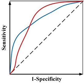
Figure 1. Two ROC curves with the same AUC value.
Download figure:
Standard image High-resolution imageTo handle the aforementioned three challenges, a unified framework termed as multifaceted radiomics (M-radiomics) was proposed for DM prediction in H&N cancer. M-radiomics deals with these challenges by introducing the following strategies:
(1) Instead of concatenating radiomic features extracted from different modalities directly, a deep learning with stacked sparse autoencoder (Hinton and Salakhutdinov 2006) is utilized to fuse the features from different modalities into one representation feature set. Autoencoder is an unsupervised learning technology developed for representation learning through a neural network (Vincent et al 2010), which has been successfully used for multimodal representation in various applications (Hong et al 2015, Ma et al 2018, Shahroudy et al 2018). As the stacked sparse autoencoder (Shin et al 2013, Xu et al 2016) can capture the joint information from different modalities (Baltrušaitis et al 2019) and increase sparsity, it is incorporated into M-radiomics for multimodal image representation.
(2) Instead of using AUC as a single objective, a multi-objective model is developed to avoid the ambiguity of maximizing AUC (figure 1). By explicitly considering sensitivity and specificity as objective functions during the model training, a preferred model with emphasis on sensitivity or specificity can be trained according to different clinical needs in the multi-objective model (Zhou et al 2019b). Furthermore, to obtain more reliable results, we designed a new probability-based objective functions to avoid the need of setting a probability threshold in classifying a prediction as positive or negative for the calculation of both sensitivity and specificity.
(3) Instead of choosing a preferred classifier, M-radiomics employs multiple base classifiers to build the predictive model. Combining different kinds of classifiers can increase the model diversity and improve its stability (Feurer et al 2015). Each base classifier in M-radiomics generates a Pareto-optimal model by employing multi-objective model. The final Pareto-optimal model set is obtained by sorting models from all the classifier-specific Pareto-optimal model sets in a non-dominated way. Since all the Pareto-optimal models are useful depending on the clinical needs, the probability outputs of all the models are fused in the testing stage.
To fuse the probability outputs from multiple models for the final prediction, a new evidential reasoning rule-based fusion (ERRF) (Yang and Xu 2013) strategy was proposed in this study, where both relative weight and reliability was introduced into the fusion process. The relative weight of individual model is frequently used during fusion process, while the reliability has not been well studied. In ERRF, the reliability is used for describing intrinsic property of the model, which greatly influences the final decision results. For example, we wish to make a decision by combining the decisions from multiple experts which is similar to classifier fusion. The relative importance (weight) of each expert is always considered when making the final decision in most situations. However, the reliability of each expert also has a great effect on the final decision. The reliability is different from the relative importance, as the reliability describes the intrinsic property of expert while the relative importance is the expert's extrinsic feature when comparing with other experts. Therefore, besides the relative importance, the reliability is designed to describe the model intrinsic property in ERRF to make a final decision.
2. Method
2.1. Overview
Before training and testing, a deep learning with stacked autoencoder strategy is designed to transform the features from PET, CT features as well as clinical parameters into one representation feature set in M-radiomics. We aim to generate a comprehensive Pareto-optimal model set through sorting classifier specific Pareto-optimal models in a non-dominated way in the training stage. The goal of testing stage is to fuse the non-zero weight models through analytic ER rule and get the final output probability. The problem formulation is described as follows.
The training stage of M-radiomics is shown in figure 2. Assume that the radiomic features and clinical parameters are denoted by  , where Mi represents the feature number for each modality and I is the modality number. Before training, an autoencoder model is generated using all the features from the different modalities, and the hidden layer is taken as the final feature set which is fed into the model, that is:

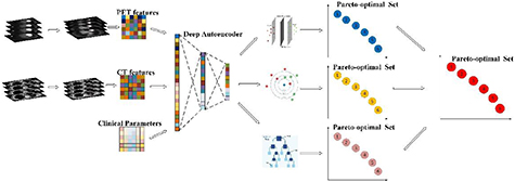
Figure 2. Illustration of the training stage of M-radiomics.
Download figure:
Standard image High-resolution imagewhere  represents stacked autoencoder and
  is the feature set generated from the hidden layer in training stage. Assume that there are N base classifiers and the model parameter set for each classifier is denoted by
  . Since the feature selection influences the model performance, we perform feature selection and model training simultaneously for each base classifier which is:

where  is the objective functions, and
  , and
, and  represent similarity-based sensitivity and specificity, respectively. After optimizing by an iterative multi-objective immune algorithm (IMIA), the classifier-specific Pareto-optimal model set
  is obtained and the final Pareto-optimal model set
  is generated as:

where  represents the non-dominated sorting strategy (Deb et al 2002). The NS strategy is used for sorting all possible solutions in the population and updating the current population to generate a new population with the same size as the initial setting.
Before performing the test as shown in figure 3, the feature set denoted by  is generated through
  . Since we hope to obtain the balanced results, models that achieve good balance between sensitivity and specificity are remained, while the other models are pruned. Assume there are M models with non-zero weight, and probability output is denoted by
  . The final output P can be obtained by fusing the M models with weight
  and reliability
  through ERRF, that is:

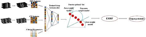
Figure 3. Illustration of the testing stage of M-radiomics.
Download figure:
Standard image High-resolution image2.2. Multimodal representation with SSAE
The features from different modalities are jointed represented through SSAE in M-radiomics. An illustration of two hidden layer stacked sparse autoencoder is shown in figure 4. SSAE (Suk et al 2015, Pan et al 2016, Zhou et al 2019a) consists of a single layer sparse autoencoder (AE) based on a neural network, which consists of an encoder and a decoder. The input vector is fed into a concise representation through connections between input and hidden layers in encoding step, while the decoding step is trying to reconstruct the input vector precisely through encoded feature representation.

Figure 4. Construction of deep learning with two layers stacked sparse autoencoder.
Download figure:
Standard image High-resolution imageAssume that x is an input vector with the D dimension containing the radiomic features and clinical parameters in our study. Then the encoder is performed by mapping x to another vector denoted by z, that is:

where h1 is a transfer function for encoder, W1 is a weight matrix and b1 is a bias vector in the first layer. The decoder is to map the encoded representation z1 back into an estimate of x, that is:

where  is a transfer function for decoder,
  is a weight matrix and
  is a bias vector in the second layer. The average output activation measure
  of
of  input vector in training set is calculated as:

where  is the number of training samples and
  represents
  training sample.
  is the
  row of the weight matrix
  and
and  is the
  entry of the bias vector. Then the sparsity denoted by
  is calculated by measuring the dissimilarity between
  and its desired value denoted by
  through Kullback–Leibler divergence (KL), that is:

By minimizing the cost function,  and
and  will be closer to each other. Additionally, it is possible that the sparsity regularizer become small with increased
  and decreased
  . To avoid this issue,
  regularization is added, that is:

where  is the number of hidden layer,
  is the number of training samples and
  is the feature number. Therefore, by adjusting the mean squared error, the cost function denoted by
  for the training sparse autoencoder is:

where  is the coefficient for
  regularization and
  is the coefficient for sparse penalty. The objective for sparse AE is to minimize the reconstruction error by optimizing above function. The SSAE is a deep learning architecture of sparse AE which can be constructed by stacking another hidden layer. Then the second hidden layer is taken as the final feature set that we will use in the next step.
2.3. Probability-based objective function
As the feature selection influences the model training, feature selection and model parameter training are performed simultaneously (Zhou et al 2017). Assume we  training samples with the label vector
 ![$T = \left[ {{T_1},{T_2}} \right]$](https://content.cld.iop.org/journals/0031-9155/65/15/155009/revision2/pmbab8956ieqn45.gif) ([1,0] for patients without distant metastasis and [0,1] for patients with distant metastasis). The model parameter set is denoted by
([1,0] for patients without distant metastasis and [0,1] for patients with distant metastasis). The model parameter set is denoted by  and the feature set is denoted by
  . In our previous model (Zhou et al 2017), sensitivity denoted by
  and specificity denoted by
  are used, and calculated them as follows:

where  is the number of true positives,
  is the number of true negatives,
  is the number of false positives, and
  is the number of false negatives.
However, the above objective functions are calculated based on the label, which may lead to less reliable results (Chen et al 2018) as the predicted output probability could be further away from the true label vector. For example, we consider a model with output of [0.9, 0.1] is more reliable than a model with output of [0.55, 0.45] as the output of the former model is closer to the ideal label vector [1,0]. In the label-based multi-objective model, sensitivity and specificity are calculated by setting the probability threshold at 0.5, which does not push the solution of output probability vector to the ideal label vector [0,1] or [1,0]. When we design a probability-based objective function without setting any threshold, we can obtain more reliable results by pushing the output probability to the ideal vector.
If we consider the label vector as a probability distribution, the problem is converted as measuring the similarity between predicted probability output and the label vector. Since Jaccard distance (Cha 2007) is an effective probability density distribution measurement, it is adopted here, that is:

where  represents the similarity measurement. The objective function becomes:

Then we define the similarity-based sensitivity and specificity, which are denoted by  ,
,  , respectively. Assume that
  represents the probability output of true positives and the corresponding labelled vector is
  . The similarity measure of true positives
  is:
is:

Similarly, we can get the similarity measure of true negatives, false positives and false negatives, which are denoted by  ,
,  and
and  , respectively. They are:
Similar to the sensitivity and specificity, we can also calculate  ,
,  :
:

Finally, the probability-based objective function is defined as:

2.4. IMIA-II
Iterative multi-objective immune algorithm (IMIA) is a multi-objective evolutionary algorithm which has shown improved performance in obtaining solutions with more balanced sensitivity and specificity as compared those single-objective bases approaches (Zhou et al 2017). However, IMIA can only handle the problem with one base classifier, while M-radiomics contains multiple base classifiers. Therefore, an enhanced version of IMIA termed as IMIA-II is developed in this work. The procedure of IMIA-II is shown as follows and a brief workflow in summarized in table 1.
Table 1. Procedures of IMIA-II.
Input: Initial population, set  |
while  , , |
| Step 1: Proportional clonal operation. |
| Step 2: Static mutation operation. |
| Step 3: Deleting operation. |
| Step 4: AUC based fast nondominated sorting approach for updating solution set. |
| End while |
| Step 5: Classifier-specific Pareto-optimal model combination and population updating. |
| Output: Pareto-optimal model set. |
Step 1—Initialization: Model parameters are optimized directly as the value is continuous. We use  to denote the maximal generation and
  denote the population, with
  as the number of individuals in one population and
  is the solution in current generation. For each base classifier, Step 2- step 5 are performed until the algorithm achieves
  .
.
Step 2—Clonal operation: Proportional cloning is used (Gong et al 2008). To diversify the population, an individual with a larger crowding-distance is reproduced more times, and the clonal time  for each individual is calculated as:
  where
where  is the expectant value of the clonal population and
  is the ceiling operator.
  represents the crowding distance.
Step 3—Mutation operation: The mutation operation (Hang et al 2010) will be performed on the cloned population . For each locus in the individual, a random mutation probability (
 ) will be generated. If
  is larger than a general mutation probability (
 ), the mutation will occur. The mutated population is denoted by
  .
.  and
and  are combined to form a new population
 .
.
Step 4—Deleting operation: If there are duplicated solutions in the new population  , we will only keep the unique one and delete other duplicated solutions. If the size of
  is less than P, step 2 should be used to generate more mutated individuals; otherwise, step 5 should be used. When the same solutions are generated in the Pareto-optimal set, the diversity of the individuals in a population will be reduced. We perform the deleting operation to ensure that all the solutions in the Pareto-optimal set are different after executing the clonal and mutation operations.
Step 5—Updating population: The selected features and model parameters for each individual are taken as the input for model (Yu et al 2005). Then,  and
and  are calculated through cross-validation. The individual in all feasible solutions is sorted in the descending order using a fast non-dominated sorting approach (Deb et al 2002) according to the AUC of each solution. We will obtain the Pareto-optimal set according to AUC because it is one of the most important criteria for the performance evaluation of a predictive model.
Step 6—Termination detection. When the algorithm reaches  , go to the next step; otherwise, go to step 2.
Step 7—Classifier-specific Pareto-optimal model combination. The final Pareto-optimal model set is generated by combining all the classifier-specific Pareto-optimal models through a AUC-based non-domainted sorting method.
Compared with traditional radiomics, more base classifiers are integrated into M-radiomics. Therefore, the main difference between these two algorithms is that IMIA-II can optimize a model with multiple base classifiers, while IMIA can only train a model with single classifier. Moreover, as each base classifier generates a Pareto-optimal model set, an additional step (Step 5 in table 1) for combining classifier-specific Pareto-optimal models is introduced into IMIA-II. As such, IMIA-II can be considered as a generalized optimization algorithm which can train the model with one or more classifiers.
2.5. ERRF-based multi-classifier fusion
Before fusing the probabilities of all the individual models through ERRF, reliability and weight are calculated. The fusion is performed through evidential reasoning (ER) rule (Yang and Xu 2013) which is a generic probabilistic inference tool and takes both relative weight and reliability into account. ER rule is a generalization of the ER approach (Yang and Xu 2002) that was originally developed for multiple criteria decision analysis based on the D-S theory (Shafer 1976). It has been applied to multiple group decision analysis (Fu et al 2015), safety assessment (Zhao et al 2016), and data classification (Xu et al 2017). However, the current ER rule is a recursive algorithm, which is difficult to perform fusion directly. Therefore, we theoretically inferred a new analytic ER rule with an analytic expression in this work.
Assume that there are  Pareto-optimal models denoted by
  with
with  classes, where
  is the output probability for a test sample
  . In our case study,
  equals 2. The reliability and weight for each individual model are denoted by
  and
and  , and the validation set is denoted by
  . Reliability is defined as the similarity between the output probability of the test sample
  and output probabilities of K nearest samples in validation set
  , that is:
where  is the output labels of test sample
  .
.  are the output labels of K nearest neighbor samples in
  , and
, and  are the corresponding output probabilities.
To better understand the reliability, we use decision making by group experts as an example. When we evaluate the reliability of an expert, a reasonable solution is that we can find several experts who have the similar background with this expert; and the reliability can be evaluated by comparing the decision result with all of other experts. In this study, as the nearest samples (e.g. K samples) of current test sample has the similar background, the reliability of each model can be evaluated through the output probabilities of these samples. Since the output probability for model  is the probability distribution, calculating the reliability of
  for test sample
  is transformed into measuring the similarity of probability distribution. Dice distance is a commonly used probability distribution measurement (Cha 2007), which is adopted here. We first define the dissimilarity among different classifiers. Assume that output probability of test sample
  is denoted by
  and output probability of one validation sample
  in K nearest neighbors is denoted by
  . The dissimilarity measure denoted by
  between test sample
  and validation sample
  is calculated as:

where  represents
  model and
  represents the
  class.
  is the
  validation sample in in K nearest validation samples. As described in equation (20), when
  ,
,  . Therefore,
  is changed as:

where  is the maximal output probability for test sample
  . Then
  is simplified as:

The similarity is then calculated as:
where  represents the similarity measurement. As there are
  validation samples, the overall similarity denoted by
  is:
is:
Assume that  (
( ) is the number of validation samples of which the output labels are the same as the test sample. Then we add
  into
into  so that it can satisfies all the constraints defined in equation (20). The reliability is then calculated as:

As predictive models are desired to have balanced sensitivity and specificity, the weight for the model with extremely imbalanced sensitivity and specificity is set as zero, whilst the weight for the remaining Pareto-optimal models are set as non-zero as shown in figure 5. As AUC is a good measurement for evaluating the model performance, it is considered for weight calculation as well. In summary, by considering the above two factors, the weight is calculated as:
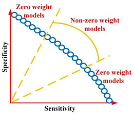
Figure 5. Pareto-optimal model with two type weights.
Download figure:
Standard image High-resolution imagewhere  ,
,  and
and  represent the similarity-based sensitivity and specificity, and AUC for model
  in training stage.
The final output probability denoted by  for test sample
  is calculated by fusing the output probabilities of all the Pareto-optimal models through analytic ER rule, that is:

where  represents analytic ER rule. The details of ER rule and the inference procedure of analytic ER rule are described in appendix A and B, respectively. After introducing analytic ER rule expression,
  is calculated as:
where the normalization factor  is:
is:

3. Experiments and analysis
3.1. Materials
In this study, FDG-PET and radiotherapy planning CT (figure 6) from 188 patients are used. All these patients had pre-treatment FDG-PET/CT scans between April 2006 and November 2017, which were downloaded from the cancer imaging archive (TCIA) (Vallières et al 2017). The follow up time ranges from 6 months to 112 months and the median follow up are about 43 months. Sixteen percent (16%) of these patients had distant metastasis. We also used clinical parameters extracted from clinical charts, including gender, age, T stage, N stage, M stage, TNM group stage. There are 257 features extracted from PET and CT images, respectively, including intensity, texture and geometry features.
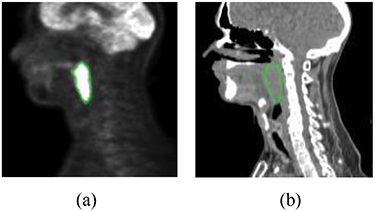
Figure 6. Illustration of FDG-PET and CT images. The green contour is the tumor: (a) FDG-PET and (b) CT.
Download figure:
Standard image High-resolution image3.2. Setup
The hidden layer size in SSAE is set as 100 based on the recommendation from reference (Guo et al 2016). Three base classifiers including radial basis function-based support vector machine (SVM), decision tree (DT) and K-nearest neighbor (KNN) are used. When training the model using IMIA-II, the population size is set as 100 and generation time is 50. The mutation rate is set as 0.9. The validation sample number K is set as 10 for reliability calculation. Five group experiments are designed as follows. (1) We compared M-radiomics with and without SSAE to see how much benefit SSAE brings. Same as most radiomics strategies, the features from different modalities are directly combined into a single vector and are fed into the model in the comparative model (without SSAE). (2) To show the improved performance when adopting multiple base classifiers, each base classifier was used for building a model and all the other setting was same as the M-radiomics. (3) We compared IMIA-II with IMIA to test the reliability of the new training algorithm. All the experimental settings were the same for these two optimization algorithms. (4) We also evaluated the reliability of ERRF strategy. Evidential reasoning-based fusion (ERF) (Chen et al 2019) and weighted fusion (WF) are used for comparison in this experiment. (5) To evaluate the overall performance, we compared M-radiomics with multi-objective (MO) radiomics model (Zhou et al 2017) and single-objective (SO) model. In MO, all the features from three modalities are concatenated into a long vector and one optimal model is selected from Pareto-optimal model. Meanwhile, SVM is used as base classifier in MO.
Five-fold cross-validation with 60% training, 20% validation and 20% testing was performed for all the experiments. AUC, accuracy (ACC), sensitivity (SEN) and specificity are used for model evaluation. Note that SEN and SPE are calculated when the cutoff value for probability output is set as 0.5. Besides these criteria, we also use similarity-based sensitivity (SIM-SEN) and specificity (SIM-SPE) to evaluate the model reliability.
3.3. Results with and without SSAE
Figure 7 shows the comparison results for M-radiomics with and without SSAE. When introducing the SSAE, M-radiomics can obtain better performance in SEN, SPE, ACC, AUC and SIM-SEN. The improved performance can be attributed to that SSAE extracts more discriminative high-level features and discovers the joint information among different modalities. The difference between SEN and SPE on the model with SSAE (0.06) is lower than the model without SSAE (0.15). Compared with the improvement on SPE and SIM-SPE, SEN and SIM-SEN are greatly improved further for the model with SSAE. These results indicate that SSAE can capture more discriminative feature such that more samples are correctly predicted for both positive and negative cases. As the dataset used in this study contains much more negative cases (84%) than positive cases (16%), greater improvement is observed in SEN and SIM-SEN than SPE and SIM-SPE.

Figure 7. Compared results for M-radiomics with and without SSAE.
Download figure:
Standard image High-resolution image3.4. Results on single and multiple base classifiers
In this experiment, we compared the single base classifier model with M-radiomics and the results are summarized in table 2. The performance of different models is compared with the paired t-test at a significance level of 0.05. The results show that there is a statistically significant difference between M-radiomics and other single-classifier-based models. Although SPE for DT is higher than M-radiomics, SEN for DT is much lower than M-radiomics. Meanwhile, SEN and SPE are highly imbalanced in DT and KNN. SVM can obtain more balanced results, but M-radiomics obtains better performance than SVM. The overall performance of M-radiomics outperforms single classifier model. The reason is that the performance of different base classifiers varies greatly for test samples with different distributions. When fusing multiple base classifiers in M-radiomics, the model diversity is greatly increased and can handle the test data with different distributions better.
Table 2. Evaluation results on three single classifiers and combined results.
| Classifier | AUC | SEN | SPE | ACC | SIM-SEN | SIM-SPE | P-value |
|---|---|---|---|---|---|---|---|
| DT | 0.82 ± 0.02 | 0.61 ± 0.03 | 0.87 ± 0.02 | 0.83 ± 0.02 | 0.94 ± 0.02 | 0.94 ± 0.03 | < 0.01 |
| KNN | 0.80 ± 0.02 | 0.59 ± 0.03 | 0.86 ± 0.01 | 0.81 ± 0.02 | 0.88 ± 0.03 | 0.91 ± 0.01 | < 0.01 |
| SVM | 0.80 ± 0.03 | 0.72 ± 0.03 | 0.78 ± 0.02 | 0.77 ± 0.02 | 0.94 ± 0.02 | 0.93 ± 0.01 | < 0.01 |
| M-radiomics | 0.84 ± 0.02 | 0.78 ± 0.03 | 0.84 ± 0.02 | 0.83 ± 0.02 | 0.98 ± 0.01 | 0.94 ± 0.03 | — |
3.5. Comparative study between IMIA and IMIA-II
This experiment is to compare the model performance after optimizing through IMIA and IMIA-II, and the results are shown in figure 8. Compared with IMIA, the model trained by IMIA-II can obtain better performance, which shows that our newly defined probability-based objective function can get a more reliable model. Specifically, IMIA-II can obtain higher AUC and SIM-SEN, which suggests that the model trained by IMIA-II is more reliable.
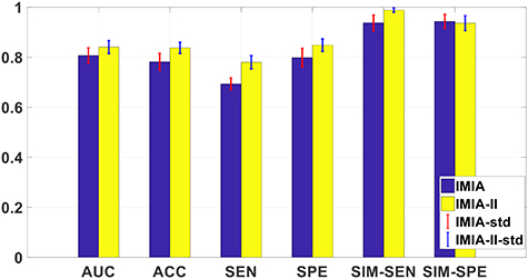
Figure 8. The reliability evaluation results for IMIA and IMIA-II.
Download figure:
Standard image High-resolution image3.6. Comparative study among three fusion strategies
We compare the model reliability when using different fusion strategies and the results are shown in figure 9. ERRF can obtain best results in six evaluation criteria among three strategies. Compared with another two strategies, the main difference of ERRF is it introduces the model reliability during the fusion process, which makes the model more reliable. Meanwhile, both ERF and ERRF outperform WF. ER is a special case of ER rule (Yang and Xu 2013), which demonstrates that ER rule is an outstanding probabilistic inference tool for information fusion.
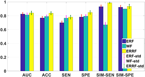
Figure 9. The reliability evaluation results for three fusion strategies.
Download figure:
Standard image High-resolution image3.7. Overall performance evaluation
The overall performance of M-radiomics is evaluated in this experiment and radiomics models with multi-objective (MO) and single objective (SO) are used for comparison. The ROC curves for SO, MO and M-radiomics on one running time are shown in figure 10. M-radiomics outperforms both SO and MO models. The average AUC for MO, SO and M-radiomics are 0.76, 0.81 and 0.84, respectively. These results demonstrate that the newly developed strategies in M-radiomics can overcome the challenges in commonly used radiomics approaches and the overall performance is improved.

Figure 10. ROC curves for M-radiomics, SO and MO.
Download figure:
Standard image High-resolution image
4. Discussions and conclusions
In this work, a unified framework, termed as multifaceted radiomics (M-radiomics), was proposed for DM prediction in H&N cancer after radiation therapy. M-radiomics overcomes three main challenges in commonly used radiomics including multimodal representation, multi-objective model optimization, and multi- classifier utilization and fusion. Since deep learning with stacked sparse autoencoder is good at multimodal representation and can catch joint information among different modalities, it was incorporated into M-radiomics to fuse the radiomic features from different modalities into one representation set. A multi-objective model with a newly designed probability-based objective function was also developed to maximize the similarity between the output probability and label vector. Furthermore, based on our previously proposed IMIA, an enhanced IMIA-II algorithm was developed to train the model. To increase the model diversity and stability, three base classifiers were used in M-radiomics. Then ERRF was developed for fusing the output probabilities of all the Pareto-optimal models. The comparative studies demonstrated that M-radiomics can obtain better performance when introducing SSAE and multiple base classifiers. Meanwhile, the model reliability is also improved when using the developed IMIA-II and ERRF. Compared with standard radiomics strategies, the overall performance of M-radiomics was greatly improved as well.
In this work, we mainly focused on predictive model construction of radiomics. However, the performance of radiomics is also affected by other aspects such as image acquisition, segmentation and feature extraction. When images are acquired at different institutions, variations of the image acquisition protocol will lead to uncertainties of feature quantification. Standardization of image acquisition protocols is desired to harmonize datasets across different institutions. The tumor contours used in this study are from the clinical target tumor of treatment plan for radiation therapy, which are manually segmented by treating physicians. While those contours are approved in clinical treatment plans, automatic segmentation is desired to minimize inter-observer variations. Furthermore, the features used in this work are extracted from segmented tumors only. Regions surrounding the tumor may additional information for DM prediction. Therefore, features extracted from tumor peripheral regions, such as shell feature (Hao et al 2018), can be incorporated into M-radiomics to further improve its performance. Finally, only hand-crafted features are used in the current M-radiomics model. Several recent studies have demonstrated that learned features and handcrafted features can be complimentary for various tasks (Li et al 2019, Lou et al 2019). As such, to fully use of all the valuable information, the features learned by deep learning can be integrated with hand-crafted radiomic features for M-radiomics.
In current M-radiomics, stacked autoencoder is employed for multimodal representation. Several new representation learning strategies have been developed recently, which may be used for multimodal representation to further improve the performance of M-radiomics (Chen et al 2020). Moreover, only three base classifiers are considered in current work. However, all the advanced classifiers can be integrated into the M-radiomics framework, such as deep learning-based classifiers and XGBoost algorithm (Chen and Guestrin 2016). In the present M-radiomics framework, the features from different sources (e.g. clinical parameters and imaging features) are jointed represented through SSAE. Alternatively, we can use a multi-task learning approach to include both imaging features and clinical feature (Guo et al 2020). For example, Guo et al proposed a new multi-task learning model for mortality prediction using low-dose CT (LDCT) images (Guo et al 2020). In this model, the overall task is divided into several subtasks, where image feature extraction and clinical measurement estimation are performed simultaneously. The learned features in the multi-task framework are jointly used when training all the subtasks. Such a strategy can be considered during the model training in M-radiomics.
The performance of M-radiomics was evaluated on a public dataset through cross-validation. Although M-radiomics outperforms several current radiomics methods, it is desired to evaluate its effectiveness on an additional dataset. We are currently constructing a dataset on H&N patients of our own institute and the performance of M-radiomics will be tested on our dataset in a future work.
Acknowledgments
The authors thank Dr Jonathan Feinberg for editing the manuscript. This work was partially supported by the US National Institutes of Health (R01 EB027898).
Appendix A.: Evidential reasoning rule
Assume that  is a set of mutually exclusive and collectively exhaustive hypotheses, where
  is referred to as a frame of discernment. So the power set of
  consists of all its subsets, denoted by
  or
or  , as follows:

where  are the local ignorance. In the ER rule, a piece of evidence
  is represented as a random set and profiled by a belief distribution (BD), as:

where  is an element of evidence
  , indicating that the evidence points to proposition
  , which can be any subset of
  or any element of
  except from the empty set, to the degree of
  referred to as probability or degree of belief, in general.
  is referred to as a focal element of
  if
if  .
.
The reasoning process is performed by defining a weighted belief distribution with reliability (WBDR) (Chen et al 2015):

where  measures the degree of support for
  from
from  with both weight and reliability being taken into account, defined as follows:

 is a normalization factor, which satisfies
  .
.  , is acting as a new weight. In the next step, the ER rule combines multiple pieces of evidence recursively. If two pieces of evidence
  and
and  are independent,
  and
and  jointly support proposition
  denoted by
  , which is generated as follows:

When there are  pieces of independent evidence, the jointly support proposition
  denoted by
  can be generated by the following two equations:


After normalization, the combined BD  is calculated as:

Appendix B. Analytic ER rule
As there's no local ignorance in our problem, they are not considered in ER rule. Therefore, the BD under no local ignorance for each evidence  is represented as:

Then WBDR is:

where  represents the class and
  is the output probability of individual classifier
  .
.  is the new weight.
Since normalization in the evidence combination can be performed in the end and does not change the results, it is applied it in the end. Assume that  and
and  denote the WBDR generated by combining the first
  evidence. The combination of two evidences with
  is considered at first. And the combined WBDR which is generated through integrating the two evidences using orthogonal sum operation are calculated as:
And

Assume that the following equations are true for the (l-1) evidences. Let  and:
and:


The above combined probability output is further aggregated with the lth evidence. So the combined probability masses are given as:
And,

In the following, the combined WBDR results are normalized. Assume that  is the normalization factor, therefore,

That is:


So,

Therefore,

where  and
and  are the combined WBDR after normalization. So the BD
  after combining l evidence is:

Based on equation (A.4) and  , the final BD is:
and  is:
is:
