Flexible numerical simulation framework for dynamic PET-MR data

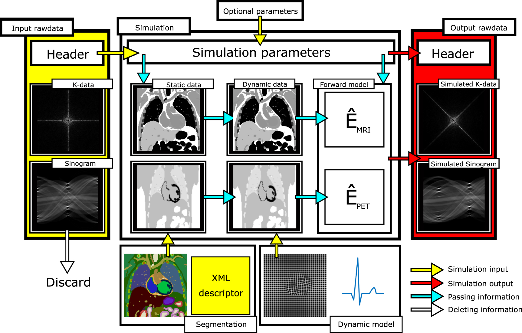
An overview of the framework design is given in figure 1. Input and output for the simulation is provided in standardised community format (ISMRMRD (Inati 2017) format https://github.com/ismrmrd/ismrmrd for MRI¹ , and Interfile for PET (Todd-Pokropek et al 1992)). The acquisition parameters (e.g. $\text{T}_\text{E}$, $\text{T}_\text{R}$, flip angle, sequence type, image resolution, number of receiver coils and k–space trajectory for MR or detector geometry for PET) are automatically set based on the header information of MR and PET raw data files. This enables and reproduction of a phantom or in–vivo scan carried out on a PET-MR scanner using the exact same hardware—and sequence–related parameters in the simulation framework, or the user can choose to overwrite them.

Zoom In Zoom Out Reset image size

During the simulation, the data part of the input file is replaced by the generated simulation data yielding a raw data output file, which is fully compatible with any image reconstruction framework capable of dealing with ISMRMRD and/or Interfile raw data. In this manner, the simulation can emulate the acquisition of already available in–vivo data while simultaneously providing GT information. Furthermore, this allows using the simulation output in already existing reconstruction workflows without modifications otherwise necessary to read and process the simulation output.

In addition to the raw data file, an anatomical segmentation combined with an XML descriptor detailing the tissue parameters for each voxel in the segmentation must be supplied. Each tissue type is characterised by $\text{T}_\text{1}$, $\text{T}_\text{2}$, spin density, chemical shift, PET tracer radioactive activity concentration and PET attenuation value which describes its MR and PET behaviour. In this study, the XCAT (Segars et al 2010) phantom was employed to generate a tissue segmentation and respiratory and cardiac motion models. However, the input format for the segmentation is vendor–independent and arbitrary voxelised anatomical segmentations and matching motion models can be used. The MR and PET scan parameters are then utilised to simulate realistic MR and PET signal intensities for the different tissue types present in the anatomical segmentation. The MR signal for each voxel is computed based on tissue parameters and sequence type using an effective signal model (Brown et al 2014). Currently, only a low flip angle FLASH contrast is available, but extensions to other sequences with a signal model available can be easily made. The PET signal assigns the activity concentration (defined in the XML descriptor) to each voxel and transforms it into specific activity (Bq) by multiplication with the voxel volume.

The signal encoding process is performed after the generation of PET and MR signal intensities. The MR raw data is generated by sampling the k–space of the three–dimensional (3D) signal. The default k–space shape and acquisition parameters are defined by the information contained in the header of the input file, but can also be changed by the user to simulate modifications to the sampling procedure. Furthermore, MR signal reception is simulated using multiple receiver coils to allow parallel imaging (Pruessmann et al 2001). Each sampled readout line is subsequently stored in the ISMRMRD data structure and written to file.

In contrast to MR, the parameters of PET raw data are defined by the geometry of the detector. This is provided by a template raw data file in Interfile format describing the desired scanner, which is currently limited to ring-shaped designs with possible future extensions to prototype architectures (Khateri et al 2019). The forward operator $\hat{E}_{\text{PET}}$ maps the activity distribution into sinogram space and includes tissue attenuation. During a simulation including motion, the motion model is applied simultaneously to the activity distribution and the attenuation map to ensure they are aligned for all simulated time points.

For MR, Gaussian noise is added to the real and imaginary part of the simulated k–space data based on an signal-to-noise ratio (SNR) parameter defined in the image as $\text{SNR} = \mathcal{S}/\sigma_n$, where $\mathcal{S}$ is the simulated signal and σ_n is the standard deviation of a complex Gaussian distribution in image space. The signal $\mathcal{S}$ in the MR image depends on sequence but also tissue–specific parameters ($\text{T}_\text{1}$, $\text{T}_\text{2}$, spin density). Therefore the user can set a reference tissue type in which the SNR is defined. This enables to simulate data with a predefined SNR in one region of the image, e.g. SNR = 15 in the liver. The noise is then added to the k–space data in Fourier space as a Gaussian distribution with a scaled width. The SNR is computed assuming data acquisition is carried out with the body coil. Therefore, using the simulation with multiple receiver coils the data will yield data with increased SNR compared to the simulation SNR parameter due to noise averaging. This has to be accounted for by the user.

The sinograms for the PET raw data given by the forward operation $\hat{E}_{\text{PET}}$ applied to the activity distribution $A({\boldsymbol r})$ describe the decay events along each line of response (LOR) per unit time. Poisson noise is added to them based on the acquisition time $\text{T}_{\text{acq}}$ defined by the user.

The framework is set up to flexibly accept arbitrarily many independent dynamic processes as input, in the following referred to as modes, which are combined into one simultaneous process during the simulation. Hence, the framework allows the inclusion of multiple four–dimensional (4D) motion models, e.g. 4D respiratory and cardiac motion as independent motion modes, that result in a data set containing cardio–respiratory motion.

To fully describe one such motion mode during the simulation, a set of motion vector fields (MVFs) describing the anatomical deformations and a motion control signal (CM) describing its temporal progression are required. The CM can be passed in the most generic format as a set of pairs (t, s) = (time–point, signal amplitude) with s ∈ [0, 1], which are interpolated onto continuous time during the simulation. Deformations must define the displacement of each voxel during the motion relative to the reference motion state given by the segmented image. The motion model must encompass all the affected organs, e.g. the entire abdomen for respiration, and must be self-consistent, such that different organs move correctly relative to each other. Anatomy and motion models available for individual organs must be combined and interpolated onto a grid matching the segmentation prior to using them as an input and must be supplied as a set of dense MVFs: ${\boldsymbol m} = \{{\boldsymbol m}_n\}, n \in \{1, \dots, N \}$ where ${\boldsymbol m}_1 = {\boldsymbol m}(s = 0)$ and ${\boldsymbol m}_{N} = {\boldsymbol m}(s = 1)$ respectively correspond to the borders of the interval on which the CM is defined. However, the number of supplied MVFs does not limit the number of simulated motion states. The simulation performs a continuous simulation of the entire motion range interpolating between the discrete motion states given by $\{{\boldsymbol m}_n\}$: for example, assume N = 3 with $\{{\boldsymbol m}_1 = {\boldsymbol m}(s = 0), {\boldsymbol m}_2 = {\boldsymbol m}(s = 0.5), {\boldsymbol m}_3 = {\boldsymbol m}(s = 1)\}$. Then the state s = 0.75 is generated using ${\boldsymbol m}(s = 0.75) = 0.5 \cdot ({\boldsymbol m}_2 + {\boldsymbol m}_3)$.

While motion deforms the anatomy, dynamic contrast modes can be included to modify the tissue parameters as a function of time, e.g. $\text{T}_\text{1}$ or activity concentration, translating into signal variation over time. Independent contrast modes can be included flexibly and are combined during the simulation to simultaneous contrast variations. As for motion, a contrast mode requires a contrast control signal (CC) describing the temporal variation of the tissue parameters. For each tissue type θ, (e.g. θ = liver) the user must define two border tissue parameter states, θ₀ = θ(s = 0) and θ₁ = θ(s = 1) and the normalised CC as pairs (t, s), s ∈ [0, 1]. Every tissue parameter θ_s can be described by a linear combination between the two border condition tissue states θ₀ and θ₁:

$$\begin{align} \theta_s = (1-s) \cdot \theta_0 + s \cdot \theta_1 . \end{align} \tag{ 1 }$$

For example to simulate the contrast changes in the liver upon injection of contrast agent, θ = liver. s = 0 means no contrast agent is in the tissue and s = 1 corresponds to the maximum concentration. For a contrast agent effecting the $\text{T}_\text{1}$ relaxation time the liver parameter in the simulation could be set up as $\text{liver}_0.\text{T}_1 = {900}\, {\rm ms}$ and $\text{liver}_1. \text{T}_1 = {300}\ {\rm ms}$. E.g. at s = 0.3 this yields $\text{liver}_{0.3}.\text{T}_1 = 0.7 \cdot \text{liver}_0.\text{T}_1 + 0.3 \cdot \text{liver}_1.\text{T}_1 = {720}\ {\rm ms}$. A dynamic behaviour is generated since s(t) is a function of time. Aside from the $\text{T}_\text{1}$ value, the contrast modes can for example also model the decay of activity over time or changes in the attenuation map linked to respiration in PET. The independent contrast dynamic modes are not limited to one tissue type, but each tissue type (i.e. liver parenchyma, blood, lesion etc) can be assigned its own contrast mode independently without computational overhead. Naturally, the simulation combines the added contrast modes with added motion modes, yielding their combined dynamic behaviour.

For MR, the time axis underlying the simulation process is defined by the timestamps of the MR template raw data. During a dynamic simulation it must be guaranteed that each readout line is acquired in the correct dynamic state defined by the simulation control signal at the readout's timestamp. In principle the above approach of interpolating the dynamic models onto a continuous time axis allows simulations with an arbitrary temporal resolution. In practice, however, only a finite number of dynamic states are simulated for computational reasons. This means that multiple time points are grouped together into a bin with a certain temporal width for contrast modes and with a certain motion amplitude for motion states. Readouts at these time points are acquired in the same dynamic state. Eventually, only one k–space is stored, whose individual points are sampled at different contrast and motion states. In most cases, motion leads to periodic changes in the anatomy which is different for contrast modes. Therefore, two alternative binning schemes are used (figure 2):

• For contrast modes the time axis is binned directly by grouping together a set of subsequent time points. The dynamic state is then defined by sampling the CC in the bin centre. This yields a unique partition of the time axis independent of the CC. Therefore contrast variations in many different tissue types can be simulated simultaneously without computational overhead.
• For motion modes, instead of the time axis, the CM axis is split into bins and the dynamic state is defined directly at their centre. The time axis binning results from grouping together time points from the same dynamic state interval. Since the same motion state occurs repeatedly throughout the simulation it is much more efficient to only apply the motion model a minimum number of times and sample the necessary k–space points depending on their timestamps. However, for each motion dynamic, an individual time axis partition must be computed. All time points corresponding to one signal bin can be simulated with a single application of the motion model (Modat et al 2010), avoiding redundant motion simulations.

Zoom In Zoom Out Reset image size

For each independent mode, their individual time axis partition is computed independently and intersected subsequently with the others to generate the simultaneous dynamic behaviour of the simulation.

For PET, however, each dynamic state is stored as an independent sinogram. The time spent in each bin defines how many counts contribute to each sinogram and hence its noise level which therefore differs between dynamic states.

Generally, for each mode the number of simulated motion states should be higher than the number of reconstructed motion states in order to accurately simulate effects such as intra-bin blurring. The suitable number of simulated states depends on the motion amplitude and should be such that the maximum amplitude in voxels divided by the number of simulated phases is below half the voxel size.

The MVFs ${\boldsymbol m}_a^b$ are defined to transform images I between motion states a and b:

$$\begin{align} &{\boldsymbol m}_a^b: \mathbb{R}^3 \rightarrow \mathbb{R}^3; I_a \mapsto I_b \end{align} \tag{ 2 }$$

$$\begin{align} &I_b({\boldsymbol r}) = I_a( {\boldsymbol m}_a^b ( {\boldsymbol r} ) ) \end{align} \tag{ 3 }$$

The framework yields one MVF for each of the N_sim simulated motion states. The set of GT MVFs are defined relative to a reference phase I₀, given by the segmentation input, and point to the simulated N_sim motion states:

$$\begin{align} & \mathcal{GT}_{sim}^\prime = \{{\boldsymbol m}_0^s \}\nonumber\\ & s \in [0,1], \; | \mathcal{GT}_{sim}^\prime | = N_{sim}. \end{align} \tag{ 4 }$$

The image reconstruction can yield a different number of dynamic states N_reco compared to the simulated ones N_sim and can also yield a different reference phase which is used in the image registration. In order to be able to compare the MVFs obtained from the reconstructed images, the GT motion information output $\mathcal{GT}_{sim}^\prime$ must be post–processed. This is discussed in more detail in the appendix in section A. To evaluate the registration output the simulation framework is able to generate regions of interest (ROIs) based on the underlying tissue segmentation for the different motion states.

All tissue segmentation and motion models were generated by the XCAT software (Segars et al 2010). A simulation of a PET-MR exam on a 3 T Siemens Biograph mMR was performed using raw data files from a patient data examination with the patient's self-navigator and ECG signal as CM input (figure 3). Continuous MR data acquisition during free-breathing was simulated for a triple-echo prototype Dixon-based GRE Golden angle Radial Phase Encoding sequence (TR = 5.9 ms, TE = 1.2/2.7/4.2 ms, FA = 10^°, #phase encoding points = $125 \frac{\text{pts}}{\text{angle}} \times 256\, \text{angles}$) (Prieto et al 2010, Kolbitsch et al 2018). The spatial resolution of MR was 1.9×3.2×3.2 mm³. The simulated coil sensitivities consisted of a simple setup of four 3D varying Gaussian profiles without phase variations between the different RF receive channels. However, more sophisticated coil map simulations or measurements from an existing scanner could be easily included and passed as a simulation parameter. The PET sinograms were simulated based on the same segmentation input as the MRI data. The forward model encoded the spatial resolution of a Biograph mMR detector using ray tracing. The individual PET images were reconstructed at different resolutions depending on the application. This is described below. Attenuation was included in the simulation but scatter and randoms effects were so–far omitted. The total acquisition time was set to match the MR scan at 3.2 min. These parameters were used for all subsequent PET simulations.

Zoom In Zoom Out Reset image size

The output of the simulation framework was reconstructed into different cardiac and respiratory motion states resulting in a series of 3D images {I_s}, s ∈ [0, 1]. To generate a motion model, this image series was registered to a reference phase $I_{s_0}$ evaluated against the GT in an ROI containing the left ventricle myocardium. Details on the post–processing procedure and definition of the registration error can be found in appendix (A and B). Using equation (B), the maximum error over all motion phases, i.e.

$$\begin{align} \Delta^{reg} = \max_s \biggl{(} \bigl{\langle} \Delta_s^{reg}({\boldsymbol r}) \bigr{\rangle}_{\text{ROI}} \biggr{)} \end{align} \tag{ 5 }$$

is computed to quantify the spatial accuracy of the registration output. Δ^reg will be referred to as the registration error in the following. When evaluating the registration error it was compared to the maximum amplitude of the GT MVFs which is the error made in neglecting motion and reconstructing the average motion. The application of a motion–compensated reconstruction can only expect to improve image quality if the motion model is more accurate than this threshold. This comparison is depicted in figures 5 and 6.

Zoom In Zoom Out Reset image size

Zoom In Zoom Out Reset image size

Zoom In Zoom Out Reset image size

3.2.1. Image registration using cardiac–resolved 4D PET

To quantitatively evaluate a registration algorithm a 4D PET dataset was simulated in 16 cardiac motion states. Eight motion states {I_t} were reconstructed at the signal locations $t = \{0.125, 0.25, \dots 1.0\}$ at a spatial resolution matching the MR reconstructions at 1.92×3.2×3.2 mm³. Attenuation correction was omitted to avoid the imprint of a static attenuation map veiling the actual motion content of the images at the cost of an apparently increased uptake in the lungs. The registration algorithm optimised an energy functional:

$$\begin{align} {\boldsymbol m}_{s}^{s_0} = \min_{\hat{{\boldsymbol m}}_{s}^{s_0}} \mathcal{E}(\hat{{\boldsymbol m}}_{s}^{s_0}) & = \min_{\hat{{\boldsymbol m}}_{s}^{s_0}} \mathcal{S}(I_s \circ \hat{{\boldsymbol m}}_{s}^{s_0},I_{s_0}) \end{align} \tag{ 6 }$$

where $\mathcal{S}$ is a similarity measure. In the case of this study, normalised mutual information was used as a similarity metric. The transformation was modelled as a free–form deformation (FFD) using B-spline interpolation (Rueckert 1999, Schnabel et al 2003) without further regularisation because these ensure a smooth motion field on the interpolation scale. The reconstructed images were registered for different spline control point distances ΔB to assess the influence of the intrinsic regularisation on the registration quality. The influence of the registration output on the image quality was assessed by summing the deformed image series:

$$\begin{align} I_{corr}({\boldsymbol r}) = \sum_{\sigma\in \{s\}}(I_{\,s_0}^{\,\sigma} \circ {\boldsymbol m}^{s_0}_\sigma)({\boldsymbol r}) \end{align} \tag{ 7 }$$

3.2.2. Synergistic registration using 4D PET-MR

Further application of the framework was the evaluation of an advanced synergistic motion estimation algorithm (Kolbitsch et al 2018). To this end two PET-MR datasets were simulated containing 4D cardiac and respiratory motion, respectively. The MR images were reconstructed using an iterative SENSE approach (Pruessmann et al 2001) for respiration and compressed sensing (CS) (Lustig et al 2007) for cardiac motion. Reconstructions yielded image series at the same motion states and with the same spatial resolution as the 4D PET data in section 3.2.1. An extended version of the image registration from equation (6) with energy functional:

$$\begin{align} \mathcal{E}({\boldsymbol m}_{\,s}^{\,s_0}) & = (1-\lambda) \cdot \mathcal{S}( I_{s}^{\,MR} \circ {\boldsymbol m}_{\,s}^{\,s_0}, I^{\,MR}_{\,s_0} ) + \lambda \cdot \mathcal{S}( I_{s}^{\,PET} \circ {\boldsymbol m}_{\,s}^{\,s_0}, I^{\,PET}_{\,s_0} ) \end{align} \tag{ 8 }$$

with I^MR/PET as the PET and MR image series relative to a phase $I^{\,MR/PET}_{s_0}$, and the synergy weight λ ∈ [0, 1] balancing the PET and MR contribution to the cost function. The synergy weighting parameter was varied in the range $\lambda \in \{0, 0.1, \dots , 0.9, 1.0 \}$ at ΔB = 12 for cardiac motion and ΔB = 24 for respiration.

All simulations were carried out using in–vivo PET-MR data as template input. Cardiac and respiratory motion were included as independent motion modes with $N_r = N_c = 8$ states respectively, yielding simultaneous cardio–respiratory motion in 64 combined motion states. This corresponded to a cardiac time interval of 125 ms at 60 bpm. Based on the cardiac and respiratory input signal the simulation output was double-binned into $N_r \times N_c = 4\times4$ motion states for both modalities, corresponding to a temporal resolution 250 ms at a motion frequency of 60 bpm. The reconstructions were performed with and without motion compensation (Batchelor et al 2005) using the ground truth motion fields. Subsequently, the resulting images were compared to corresponding reconstructions of the in-vivo patient data to verify that the proposed framework yields realistic output data. The PET images were reconstructed at a resolution of 2×2.1×2.1 mm³ matching the patient data used in the comparison. The MR simulation data were reconstructed using an iterative SENSE approach (Pruessmann et al 2001). For PET attenuation correction (AC) during reconstruction a static attenuation map used as the simulation input was employed. For a more detailed description of the employed motion–correction scheme, please refer to Kolbitsch (2017).

3.4.1. Data acquisition

3.4.2. Quantitative parameter estimation

An extended Toft's model for the temporal evolution of the gadoxeate disodium concentration in the tissue of interest (TOI) $\mathcal{C}_{toi}(t)$ was fitted based on an arterial input function (AIF) extracted from the hepatic artery in the template data (Ippoliti et al 2019):

$$\begin{align} \mathcal{C}_{toi}(t) = v_p \cdot \mathcal{C}_p(t) + k_{trans} \cdot \mathcal{C}_p(t - \Delta T) * e^{- \frac{k_{trans}}{v_e}t}, \end{align} \tag{ 9 }$$

with $\mathcal{C}_p$ the blood plasma contrast uptake, v_p the volume fraction of blood plasma, v_e the extravascular extracellular fractional volume, k_trans the volume transfer constant, ΔT the time delay of tissue enhancement with respect to the arterial concentration in plasma and * representing the convolution operator. Every parameter of the right–hand side of equation (9) depends on TOI except $\mathcal{C}_p$. The simulated tissues of interest were healthy liver tissue and a hepatic lesion with a necrotic core. The parameters used as simulation input can be found in table 1. The necrotic core was simulated as lesion tissue without any contrast agent kinetics. The resulting Toft's model and simulated $\text{T}_\text{1}$ variations are depicted in figure 4.

Table 1. Input parameters employed in the Toft's model described in equation (9).

Tissue type	Healthy Liver	Lesion	Lesion Core
ktrans	0.041	0.135	0
vp	0.025	0.141	0
ve	0.087	0.022	1
ΔT[min]	0.19	0.20	0

The concentration of contrast agent was converted into a temporal evolution of $\text{T}_\text{1}$ using $T_1(t) = \frac{1}{R_1(t)} = \frac{1}{R_1 + r \cdot \mathcal{C}_{toi}(t) }$ where r = 6.2 mmol s⁻¹ is the relaxivity of Primovist at 3 T (Rohrer et al 2005). The simulated Toft's model and the calculated change in the $\text{T}_\text{1}$ parameter extracted from patient data used as simulation input is depicted in figure 4.

The DCE simulation was performed for N_r = 16 respiratory states and N_c = 49 contrast states.

3.4.3. Image reconstruction and impact of motion field inaccuracies

From the simulation output a k–t–SENSE reconstruction was performed with and without respiratory motion correction (Batchelor et al 2005). In order to assess, how inaccuracies in the motion estimation would impact the assessment of the quantitative parameters such as k_trans, a bias of different strength σ was added to the GT motion fields using:

$$\begin{align} \mathcal{GT}_{\sigma} = \{{\boldsymbol m}_{\sigma}^{t} \} = {\boldsymbol m}_{0}^{t} + \sigma \cdot \frac{t}{N_{reco} - 1} \cdot {\boldsymbol n} \end{align} \tag{ 10 }$$

where ${\boldsymbol m}_{0}^{t}$ are the GT MVFs for reconstructed motion phase $t\in \{0 \dots N_{reco}-1\}$, σ is the bias strength, $\sigma \in \{0, \dots, 6 \}$ and ${\boldsymbol n}$ a spatially varying (but temporally constant) random unit vector field which fixes the direction of the bias for each voxel. This random unit vector was not drawn for each voxel independently, but on a larger grid and subsequently spline-interpolated to the resolution of the motion fields. This procedure took into consideration that the image registration algorithm used here is spline-based, and hence errors in the motion estimation are expected to vary smoothly between neighbouring voxels. The increase of bias with each reconstructed motion phase included potential accumulation of error with increasing registration amplitude in registration. Each of the motion field sets $\mathcal{GT}_{\sigma}$ were then used in the motion–corrected reconstruction and k_trans maps were computed from the dynamic contrast–resolved image time series. The between lesion and necrotic core for uncorrected and motion-corrected (with different values for σ) images was compared. CNR was computed as $\text{CNR} = \frac{\mathcal{S}_{\text{lesion}} - \mathcal{S}_{\text{core}} }{\sigma_{\text{lesion}}}$ where $\mathcal{S}_i$ and σ_i are the mean and standard deviation of the k_trans maps in the respective tissue regions. These were evaluated in a 2D axial slice through the lesion centre and segmented by hand.

4.1.1. Image registration using cardiac–resolved 4D PET

4.1.2. Synergistic registration using 4D PET-MR

Images reconstructed from the simulated PET-MR raw data are compared to the corresponding in–vivo patient data in figure 7. Respiratory and cardiac motion leads to similar motion artefacts in both datasets for PET and MR. In the MR images blurring of anatomical structures such as the heart or the liver can be clearly seen for both in–vivo data and numerical simulations. The PET images show blurring of the myocardium and papillary muscles. Motion correction of respiratory and cardiac motion in the in-vivo data improves the image quality, leading to a better depiction of the anatomy comparable to the motion-free reference image obtained with the simulation framework.

Zoom In Zoom Out Reset image size

The reconstructed DCE images are pictured in figure 8 for both simulation and patient data. For the two datasets both respiration averaged and motion compensated k–t–reconstructions are compared in selected phases. An ROI containing a lesion with a necrotic core is zoomed in on. The slice showing the respiration average has been selected to show the same anatomical region as the respiratory–compensated images. For the selected ROI the k_trans parameter of a Toft's model fit to the DCE images is depicted. In simulation and patient data motion compensation improves the visualisation of the necrotic core of the lesion with lower k_trans value compared to the lesion itself. In the k_trans maps computed from motion–averaged cases the necrotic core is strongly blurred.

Zoom In Zoom Out Reset image size

This finding is confirmed quantitatively by the results shown in figure 9. The left plot shows the deviation from the true motion for the different σ values of the maximum respiratory amplitude. Only the configuration of σ = 6 has a deviation larger than the GT amplitude marked by the dotted line. Upper right: the CNR in the k_trans fits between lesion and core as a function of MVF bias. A non–linear relationship is revealed resulting in a decrease in CNR between lesion and necrotic core in the k_trans. A ROI–averaged bias larger than 4 mm yields a reduced CNR, in which the core is not visible any more. Deviations larger than 5 mm yield a CNR of the same magnitude as if no motion compensation had been employed (indicated by the dotted line). The k_trans maps for the different bias strengths in which the CNR was evaluated are shown below the quantitative plots. While one can see a degradation in contrast for growing bias, between σ = 0 and σ = 3 the core stays clearly outlined.

Zoom In Zoom Out Reset image size

For most applications the precision of the registration output $\mathcal{REG}$ is only of interest in a certain region (ROI). However, in a MVF the motion of a voxel is not encoded in the voxel itself but rather at the location where it is going to be deformed to (cf equation (3)). Hence, the inverse MVF encodes the motion of the voxel. To compute the registration error both $\mathcal{GT}$ and $\mathcal{REG}$ must be inverted and evaluated in the ROI:

$$\begin{align} \Delta^{reg}_s(\text{ROI}) & = \lVert ({\boldsymbol m}_s^{s_0} - \tilde{{\boldsymbol m}}^{s_0}_s)(\text{ROI})\rVert_2. \end{align} \tag{ A4 }$$

The precision of the inversion algorithm can be set arbitrarily small, such that its effect is negligible on the accuracy of the registration output². Since the registration output must be inverted eventually, in practice the inverse is registered directly: $\mathcal{REG} = \{\tilde{{\boldsymbol m}}_{s}^{s_0}\}$. Note that the ROI must be deformed from the reference phase of the segmentation into the motion state to which the dynamic images were registered: $\text{ROI}_{s_0}({\boldsymbol r}) = \text{ROI}_0( {\boldsymbol m}_0^{s_0}({\boldsymbol r}))$.