Abstract
While the pursuit of better time resolution in positron emission tomography (PET) is rapidly evolving, little work has been performed on time of flight (TOF) image quality at high time resolution in the presence of modelling inconsistencies. This works focuses on the effect of using the wrong attenuation map in the system model, causing perturbations in the reconstructed radioactivity image. Previous work has usually considered the effects to be local to the area where there is attenuation mismatch, and has shown that the quantification errors in this area tend to reduce with improved time resolution. This publication shows however that errors in the PET image at a distance from the mismatch increase with time resolution. The errors depend on the reconstruction algorithm used. We quantify the errors in the hypothetical case of perfect time resolution for maximum likelihood reconstructions. In addition, we perform reconstructions on simulated and patient data. In particular, for respiratory-gated reconstructions from a wrong attenuation map, increased errors are observed with improved time resolutions in areas close to the lungs (e.g. from 13.3% in non-TOF to up to 20.9% at 200 ps in the left ventricle).
Export citation and abstract BibTeX RIS

Original content from this work may be used under the terms of the Creative Commons Attribution 3.0 license. Any further distribution of this work must maintain attribution to the author(s) and the title of the work, journal citation and DOI.
1. Introduction
The emergence of the first time of flight (TOF) positron emission tomography (PET) scanners brought a whole new dimension to nuclear imaging, by incorporating within the PET image reconstruction the time information from a coincidence pair to estimate more accurately the localisation of the originating annihilation event. The reconstruction problem is better determined and therefore less ill-posed, accomplishing an overall better image quality and better quantification (Conti 2011). Vendors and research teams are now improving the physical characteristics of their scanners in order to get better time resolution (Lecoq 2017, Cates and Levin 2018). Current PET scanners with TOF capabilities used in clinical settings have TOF resolution between 210 ps (van Sluis et al 2019, Pan et al 2019) and ≈ 550 ps (Bettinardi et al 2011, Rausch et al 2015), but sub-100 ps time resolutions are expected in the future. A current initiative is hoping to achieve 10 ps resolution (Lecoq 2017, The 10 ps Challenge committee 2019), which would possibly allow 'reconstruction-less' PET images, as the detected events could be placed directly in the images. However, effects such as photon attenuation and scatter will still have to be taken into account.
Attenuation is defined as the loss of coincidences resulting from the photon interactions occurring within the body of the patient. Whereas photon attenuation is the foundation of x-ray imaging, it represents a major issue in PET where the fraction of photons attenuated in a tissue is proportional to the tissue density and the distance travelled through medium. For large patients, the fraction can be up to 95% and needs to be accounted for (Mettler Jr and Guiberteau 2018). In practice, this requires an attenuation map (also referred as µ map). All current scanners are in fact dual modality: they are either combined with a CT gantry (PET/CT) or with a MRI gantry (PET/MR). In this case, the PET attenuation maps are in most cases derived from the coupled modality. A CT acquisition can usually provide quite accurate information to derive the attenuation factors used in the PET image reconstruction, usually via rescaling the CT attenuation values to PET 511 keV photon energy (Kinahan et al 1998, Alessio et al 2004) (although problems exist, e.g. metal artefacts, see Blodgett et al (2011)). MR-derived attenuation maps are usually less robust (Lillington et al 2019).
Another common cause of mismatch between the estimated and actual attenuation map is motion (Bousse et al 2016). Mismatched data are common, especially in case of respiratory motion: errors can be large when no motion correction/gating is used, although intra-gate motion is unavoidable.
The use of 'mismatched' attenuation maps in the PET reconstruction can induce large quantification errors in the reconstructed images, as discussed theoretically in Bai et al (2003), Thielemans et al (2008), Ahn et al (2014) and clinically in Geramifar et al (2013), Nyflot et al (2015) and Mehranian and Zaidi (2015).
In the lungs, the attenuation mismatch is not solely due to the 'displacement' caused by the compression and dilation, but also to the change of density while doing so. Cuplov et al (2018) has shown that up to 17.1% of mass density changes can be observed during respiration. The effect of motion mismatch in the lungs was assessed in Holman et al (2016) specifically for non-TOF reconstructions and demonstrated the importance of the density changes for quantification, additionally to the effect of mis-alignment due to motion displacement. Strategies to mitigate this exist (outside of correcting for motion), such as the use of average CT images for attenuation correction (Pan et al 2005).
In non-TOF reconstruction (i.e. when the time information is not used), when far away from the edges, for an 'emission object' that is large enough (for example, in the chest), the effect is mostly local and depends on the size of the perturbation area, as well as the amount of activity in the surrounding areas. This was used to derive approximations to quantify the error in the reconstructed PET image in the area where the mismatch occurs (Thielemans et al 2008, Bousse et al 2017). In Ahn et al (2014), the effect of mismatched attenuation maps in TOF reconstruction was also considered as local, which allowed the authors to obtain an approximation of the quantification errors. Under that assumption, if the object size is considered negligible compared to the time resolution, an estimation close to the one found in Thielemans et al (2008) can be found, now depending on the time resolution instead of the size of the emission object. In both cases, only the local effect of a perturbation in the attenuation map on the emission image was considered in the analysis.
This work aims to demonstrate the non-local effect of attenuation mismatches in the reconstructed PET images for high time resolution scanners, with a focus on Maximum Likelihood Expectation Maximisation (MLEM) and Ordered Subset Expectation Maximisation (OSEM) reconstructions. Particular attention will be given to non-local errors in quantification, i.e. in regions where there is no attenuation mismatch.
The paper will first briefly introduce mathematically the reconstruction problem in PET, including a demonstration of the non-local effect and its quantification error for perfect time resolution. Then, it will show the spatial extent of a localised attenuation mismatch in the reconstructed images for different time resolutions. Finally simulations and the reconstruction of patient data will demonstrate the quantification error that can arise from the use of mismatched data. The convergence rates will also be assessed in both cases.
2. Theory
2.1. PET imaging system
The measured data take the form of a random vector  , where
 ![$[\boldsymbol{g}]_i$](https://content.cld.iop.org/journals/0031-9155/65/8/085009/revision2/pmbab7a6fieqn2.gif) is the number of counts at bin
is the number of counts at bin ![$i \in \left[\kern-0.15em\left[ {1,{n_{\rm{b}}}} \right]\kern-0.15em\right]$](https://content.cld.iop.org/journals/0031-9155/65/8/085009/revision2/pmbab7a6fieqn3.gif) and
and  is the number of detection bins.
  depends on the PET system, i.e.
  for non-TOF PET and
  for TOF PET,
  and
and  denoting the number of detection bins for non-TOF reconstruction and the number of temporal bins, respectively. The imaging system is usually modelled as

where ![$\boldsymbol{p} = \mathbb{E}[\boldsymbol{g}]$](https://content.cld.iop.org/journals/0031-9155/65/8/085009/revision2/pmbab7a6fieqn10.gif) ,
,  is the unknown emission image,
  is the imaging system matrix,
  is the background term (comprising randoms and scatter), and
  is the number of voxels.
Each entry ![$[\boldsymbol{M}]_{i,j} = M_{i,j}$](https://content.cld.iop.org/journals/0031-9155/65/8/085009/revision2/pmbab7a6fieqn15.gif) represents the probability that a pair of unscattered photons emitted in a voxel j is detected at the detection bin i, and incorporates the attenuation. In principle, detector blurring should be modelled after attenuation; however, for simplicity, we will consider the factorisation of
represents the probability that a pair of unscattered photons emitted in a voxel j is detected at the detection bin i, and incorporates the attenuation. In principle, detector blurring should be modelled after attenuation; however, for simplicity, we will consider the factorisation of  as Leahy and Qi (2000)

where  is a
is a  diagonal matrix containing the attenuation factors corresponding to
  and
and  is a system matrix that incorporates a geometrical mapping between the source and the data—each entry
 ![$[\boldsymbol{H}]_{i,j} = H_{i,j}$](https://content.cld.iop.org/journals/0031-9155/65/8/085009/revision2/pmbab7a6fieqn21.gif) represents the probability that an emission from voxel j is detected by the detection bin i in the absence of attenuation.
represents the probability that an emission from voxel j is detected by the detection bin i in the absence of attenuation.
The background term  includes scatter, which in practice can be estimated from the attenuation map (Watson et al 1996, Ollinger 1996). In the remainder of this section, we will assume that
  , so that (1) becomes

This can be achieved, for example, by subtracting  from
from  and zeroing the negative values.
2.2. Spatial extent of activity errors due to local attenuation mismatch
We assume the true activity and attenuation images are respectively  and
and  . Furthermore, we assume that
  is full rank with
  such that the mapping
  is injective. The transmission system matrix—used to generate the attenuation coefficients—is the discretised line integral operator
  .
.
The attenuation coefficient diagonal matrix  is of size
  (in non-TOF PET,
  ) and for each bin detector pair
 ![$d \in {\rm{ }}\left[\kern-0.15em\left[ {1,{n_{\rm{d}}}} \right]\kern-0.15em\right]$](https://content.cld.iop.org/journals/0031-9155/65/8/085009/revision2/pmbab7a6fieqn35.gif) and time bin
and time bin ![$t \in {\rm{ }}\left[\kern-0.15em\left[ {1,{n_{\rm{t}}}} \right]\kern-0.15em\right]$](https://content.cld.iop.org/journals/0031-9155/65/8/085009/revision2/pmbab7a6fieqn36.gif) , the diagonal element at the detection bin [id = AB]
, the diagonal element at the detection bin [id = AB] 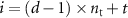
 is
is
that is to say, in TOF PET, the attenuation coefficients are independent of the time bin.
Let  be an idealised noiseless measurement of the true activity
  with attenuation
  , i.e.

In absence of noise, the PET image reconstruction problem becomes

and has a unique solution  .
.
Now assume that the attenuation map  used for reconstruction is a perturbed version of
  , i.e.
  where
where  is a small perturbation supported on a small region far from the edges. The reconstruction problem (5) is equivalent to solving
Non-TOF PET:
Along the lines of Thielemans et al (2008) and Bousse et al (2017), using a Taylor expansion around  , the problem is approximated in non-TOF PET as:

where ![$\mathrm{diag}[\cdot]$](https://content.cld.iop.org/journals/0031-9155/65/8/085009/revision2/pmbab7a6fieqn48.gif) is the operator that generates a diagonal matrix from a vector. In non-TOF, the PET system matrix
is the operator that generates a diagonal matrix from a vector. In non-TOF, the PET system matrix  and transmission matrix
  are equal. Furthermore,
  is sparse and its non-zero entries correspond to the lines of responses i intersecting the support of
  . Assuming that
  is approximately constant where
  is non-zero (this is the case, for example, when the perturbation is located far from the body contour), we can further approximate (6) as

where ρ is the mean projected activity along the lines of response intersecting the support of  . Approximation (7) shows that when
  and
and  differ from a local perturbation
  , then, by injectivity of
  , the solution to the approximated reconstruction problem is
  , which suggests that the error in the reconstructed activity remains localised on the mismatch.
TOF PET:
Equation (6) can be extended to TOF PET, i.e. for all line of response i intersecting the support of  and for all time bin t,

Approximation (8) implies that for all lines of response i intersecting the mismatch area, the error between the reconstructed activity  and
and  propagates to each time bin t by a factor proportional to
 ![$[\boldsymbol{R} \boldsymbol{\eta}]_d$](https://content.cld.iop.org/journals/0031-9155/65/8/085009/revision2/pmbab7a6fieqn64.gif) , which means the error can no longer be considered local.
, which means the error can no longer be considered local.
The previous equation (8) implies that in most cases the system to solve is made of inconsistent equations. For this reason, the solution depends on the cost function used for solving such reconstruction problem.
2.3. Maximum-likelihood expectation maximisation in perfect time resolution
In this section we deepen the analysis from section 2.2 by investigating the effect of the attenuation mismatch from the perspective of MLEM reconstruction. We will consider the highly idealised case of perfect spatial resolution here.
We denote for ![$(i,j) \in \left[\kern-0.15em\left[ {1,{n_{\rm{b}}}} \right]\kern-0.15em\right] \times \left[\kern-0.15em\left[ {1,{n_{\rm{v}}}} \right]\kern-0.15em\right]$](https://content.cld.iop.org/journals/0031-9155/65/8/085009/revision2/pmbab7a6fieqn65.gif) (here i is a TOF bin and
(here i is a TOF bin and  ):
):
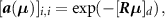
![$\widehat{\boldsymbol{\lambda}} = \left[\widehat{\lambda}_j\right]$](data:image/png;base64,iVBORw0KGgoAAAANSUhEUgAAAAEAAAABCAQAAAC1HAwCAAAAC0lEQVR42mNkYAAAAAYAAjCB0C8AAAAASUVORK5CYII=) the activity image reconstructed with the true attenuation map , i.e. using .
the activity image reconstructed with the true attenuation map , i.e. using .- the activity image reconstructed with a wrong attenuation map , where .
![$\widehat{\boldsymbol{\lambda}} = \left[\widehat{\lambda}_j\right]$](https://content.cld.iop.org/journals/0031-9155/65/8/085009/revision2/pmbab7a6fieqn67.gif)

![$\boldsymbol{M}^\star = \left[M^\star_{i,j}\right] = \boldsymbol{a}(\boldsymbol{\mu}^\star)\boldsymbol{H}$](https://content.cld.iop.org/journals/0031-9155/65/8/085009/revision2/pmbab7a6fieqn69.gif)
![$\widetilde{\boldsymbol{\lambda}} = \left[\widetilde{\lambda}_j\right]$](https://content.cld.iop.org/journals/0031-9155/65/8/085009/revision2/pmbab7a6fieqn70.gif)

![$\widetilde{\boldsymbol{M}} = \left[\widetilde{M}_{i,j}\right] = \boldsymbol{a}(\widetilde{\boldsymbol{\mu}})\boldsymbol{H}$](https://content.cld.iop.org/journals/0031-9155/65/8/085009/revision2/pmbab7a6fieqn72.gif)
We also define the sets

In a hypothetical case of an activity image reconstructed with perfect time resolution as well as perfect spatial resolution, the  are disjoint, so that

In other words, ![$[\boldsymbol{M}]_{i,j}$](https://content.cld.iop.org/journals/0031-9155/65/8/085009/revision2/pmbab7a6fieqn74.gif) is non-zero if and only if
is non-zero if and only if  . Given a system matrix
  , which can either be
  or
or  , and the measurement data
 ![${\bf{p}} = {\{ {p_i}\} _{i \in \left[\kern-0.15em\left[ {1,{n_{\rm{b}}}} \right]\kern-0.15em\right]}}$](https://content.cld.iop.org/journals/0031-9155/65/8/085009/revision2/pmbab7a6fieqn79.gif) , the MLEM algorithm (k + 1)-th iteration at a voxel j is
, the MLEM algorithm (k + 1)-th iteration at a voxel j is
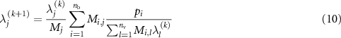
where  and
and  is the value of the activity image at a voxel j and iteration k (Dempster et al 1977, Shepp and Vardi 1982, Lange and Carson 1984).
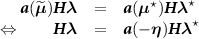
In TOF PET, assuming the temporal resolution is perfect, condition (9) holds and therefore  . Equation (10) simplifies to
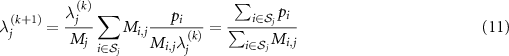
and convergence is achieved after one iteration. Substituting  with
with  and
and  successively in (11) leads to
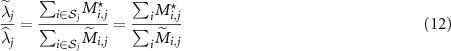
where the second equation follows from the fact that the  are disjoint. Therefore, the ratio between the 'wrong' and 'true' reconstructed images is equal to the ratio of the 'true' and 'wrong' sensitivity images. The quantification of the non-local effect due to a local error in the attenuation map, from equation (8) can therefore be quantified easily for MLEM/OSEM in the case of perfect time resolution by the relative error
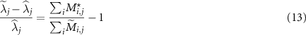
The maximum-likelihood (ML) solution being unique in this case, equations (12) and (13) are valid for other ML algorithms. It is worth noticing that for small attenuation mismatches and using the same first-order Taylor expansion around  , (13) resembles an image space version of (8). Similar results for other reconstruction algorithms are shown in the appendix.
3. Experiments and results
In this section we will study the quantification errors in TOF reconstruction due to attenuation mismatch for MLEM/OSEM.
3.1. Summary of simulated and patient data
We use four different datasets, either simulated for or acquired on a GE Discovery 690 PET/CT scanner (Bettinardi et al 2011). The PET reconstructions use two different attenuation maps: the true attenuation map  and a wrong attenuation map
  .
.
3.1.1. Simulations
The simulated datasets are the following:
Simulation 1:
A 28.8-cm diameter uniform cylinder (linear attenuation: 0.091 6 cm−1) is placed at the centre of the FOV. The wrong attenuation map  is known accurately in the reconstruction except for one small cylinder (diameter = 6 mm) at the centre of the FOV, where the attenuation is overestimated by 15%. This simulation is aimed at studying the impact of a very small attenuation mismatch on the reconstructed activity image. The phantom volumes are shown in figure 1.

Figure 1. Simulation 1 – Axial and coronal views of the input images used: (a) true activity, (b) true attenuation and (c) incorrect attenuation.
Download figure:
Standard image High-resolution imageSimulation 2:
An XCAT PET/CT simulation of an FDG oncological pulmonary acquisition at end-inspiration (tumour of 1 cm3 situated in the lower right lung). Two incorrect input  maps are assessed:
- Lung density changes only: The incorrect map (denoted ) is aligned with the structures in the PET data, however the density in the lung is not known accurately (overestimation of 15%). Note that the lung tumour density does not change, as the structure is considered rigid. Such simulation is relevant in motion-compensated image reconstruction (MCIR) or gated reconstruction, when a static map is warped to another respiratory gate (for which intra-motion is negligible), but the changes in density are not considered.
- Lung density changes + misalignment: The incorrect map (denoted ) corresponds to the end-expiration state, therefore both structure alignment and lung density are wrong. The input simulation images are given in figure 2.


Figure 2. Simulation 2 – Axial and coronal views of the input images used: (a) true activity  , (b) true attenuation
  , (c) incorrect attenuation
  , (d) absolute difference between
  and
and  (e) incorrect attenuation
  and (f) absolute difference between
  and
and  .
.
Download figure:
Standard image High-resolution image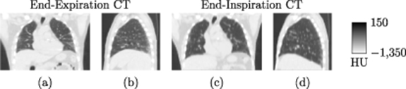
Figure 3. Patient Data – (a) Coronal and (b) sagittal view of the end-expiration CT image and (c) coronal and (d) sagittal view of the end-inspiration CT image, used to derive the attenuation maps in this study.
Download figure:
Standard image High-resolution imageData generation:
The simulations were performed using STIR with TOF (Efthimiou et al 2018) in the following order:
- Forward projection of the true activity image to obtain the non-attenuated projection data.
- Calculation of the attenuation coefficient sinogram from the true attenuation map and multiplication by the projection data.
- Reconstruction of the attenuated projection data using either the true attenuation map or the incorrect attenuation map .


To assess the effect of varying time resolution in the TOF reconstruction, the overall scanner geometry of the GE PET/CT Discovery 690 was used, but the TOF characteristics were altered:
- The maximal number of TOF bins extended to 175 (of width equal 28 ps) instead of the original 55 bins (of width ≈ 89 ps).
- The time resolution was modified to test a range of time resolutions, from 70 ps to 550 ps.
Image reconstruction:
For the simulations, the projection data were reconstructed with MLEM (image size: 256 × 256 × 47, voxel size: 2.130 6 × 2.130 6 × 3.27 mm3, no post-filter applied), using a sufficient number of iterations so that the mean difference between the last two iterations was less than 0.1% overall, when the correct attenuation map was used in the reconstruction. The numbers of iterations for the TOF reconstructions, depending therefore on the time resolution, are given in table 1. 1600 iterations were used in non-TOF reconstructions. For computational reasons, TOF 'mashing' was used in this work, therefore combining TOF bins together with only small loss reported for quantification (Efthimiou et al 2018).
Table 1. Time resolution FWHM simulated and the corresponding number of MLEM iterations used.
| TOF FWHM | 70 | 100 | 150 | 200 | 250 | 300 | 350 | 400 | 450 | 500 | 550 |
| MLEM iteration # | 80 | 160 | 160 | 240 | 240 | 240 | 240 | 240 | 240 | 240 | 240 |
3.1.2. Patient data
A 76-year-old male patient (clinical trial ID: NCT02 885 961) underwent a static FDG acquisition (injected activity: 170.8 MBq), on a GE Discovery 690 at the Institute of Nuclear Medicine, University College London Hospital (London, UK). Two different CT acquisitions were available: one at end-expiration (CTAC acquisition, multislice helical acquisition at shallow breathing, slice thickness: 3.75 mm, pitch: 1.375, voltage: 120 kVp, current: 40 mA, revolution time: 0.8 s) and one at end-inspiration (HRCT, multislice helical acquisition at breathhold, slice thickness: 1.25 mm, pitch: 0.516, voltage: 120 kVp, current: 149 mA, revolution time: 0.6 s). In addition, the listmode data were also (amplitude-) gated into 4 respiratory bins (no cardiac gating) based on the respiratory trace from a Varian RPM system. The end-expiration gated PET data were reconstructed using two µ maps  and
and  , computed from the end-expiration and the end-inspiration CT images, respectively. The alignment between the end-expiration PET data and CT image was visually assessed using non-attenuation-corrected (AC) TOF gated images. The patient data were reconstructed using GE proprietary software in MATLAB (Matlab 2016b), with OSEM using 8 subsets with 200 iterations for non-TOF data and 100 iterations for TOF data. A 2D Gaussian postfilter of FWHM 6 mm and a 1-4-1 weighted z-axis postfilter were applied to the final images (image size: 256 × 256 × 83, voxel size: 2.734 4 × 2.734 4 × 3.27 mm3).
3.1.3. Measures
At a given time resolution, we denote  and
and  the reconstructed images at the final reconstruction iteration, using the true attenuation map
  and the incorrect attenuation map
  , respectively. In the following, we will use the relative errors in absolute value defined in a region of interest (ROI)
  as
as
where  designates the mean value in
  .
.
We also define the relative difference image  (in absolute values) such that
3.2. Results
3.2.1. Simulation 1
We consider five rectangular ROIs (4 × 4 × 45 voxels, the first and last slices are excluded). The first one is placed at the centre of the field of view (FOV), therefore at the centre of the perturbation area. The four other ROIs are off-centre (distance between the centre of the FOV and the ROIs: 12.8 mm, 21.3 mm, 29.8 mm and 55.4 mm respectively). In order to minimise problems related to discretisation, off-centre ROIs measures average values in reconstructed images rotated about the centre of the cylinder (60 rotation angles considered).
We computed the relative error within the perturbation area and in the four off-centre ROIs. The plots showing the relative errors with respect to the time resolution are shown in figure 4, where the relative error at perfect time resolution was predicted by equation (13).
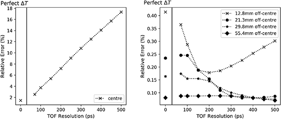
Figure 4. Simulation 1 – Relative errors versus time resolution at the centre of the cylinder (left) and for three off-centre ROIs (right), from the reconstructions and from equation (13). We used two subplots due to scale differences.
Download figure:
Standard image High-resolution imageThe first subplot is consistent with previous results on TOF, where improved time resolution decreases errors locally in the activity images. The second subplot confirms that the errors propagate globally in the image, in agreement with equation (8).
3.3. Simulation 2: lung XCAT simulation
3.3.1. Lung density changes only
In figure 5, the relative errors are plotted in different 3 × 3 × 3 voxel ROIs (left and right lungs, descending aorta and lung tumour), relative to time resolution. Similarly as for Simulation 1, the relative errors within the lungs (where the attenuation mismatch is located) decrease with improved time resolution. However, the errors increase in the lung tumour and the descending aorta. The same behaviour was observed for the right and left ventricles, as well as ascending aorta (results not shown). The results show the propagation of the errors outside of the lungs (where the attenuation mismatches lie), in neighbouring regions, as predicted by Formula (13).

Figure 5. Simulation 2 (Lung density changes only) – Relative errors versus time resolution in different ROIs: left lung, right lung, lung tumour and descending aorta.
Download figure:
Standard image High-resolution imageThe relative difference images corresponding to different time resolutions are shown in figure 6.
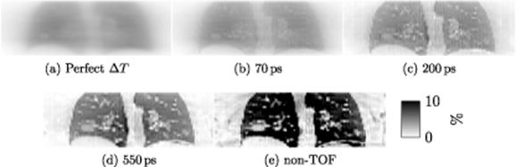
Figure 6. Simulation 2 (Lung density changes only) – Relative difference images  , in coronal view (a) expected at perfect time resolution and for four reconstructions with different TOF resolution: (b) 70 ps, (c) 200 ps, (d) 550 ps and (e) non-TOF.
Download figure:
Standard image High-resolution image3.3.2. Lung density changes + misalignment
In figure 7, the relative difference images in absolute values are shown.
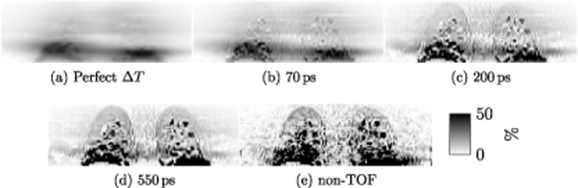
Figure 7. Simulation 2 (Lung density changes + misalignment) – Relative difference images  , in coronal view (a) expected at perfect time resolution and for four reconstructions with different TOF resolution: (b) 70 ps, (c) 200 ps, (d) 550 ps and (e) non-TOF.
Download figure:
Standard image High-resolution imageAdditionally, the relative errors  were quantified in different ROIs
  : ascending aorta (AA), descending aorta (DA), left ventricle (LV), right ventricle (RV) and liver. The relative differences
  between
  and
and  are given in table 2.
Table 2. Simulation 2 (Lung density changes + misalignment) – Relative errors  for different time resolutions and for non-TOF in different ROIs
  : ascending aorta (AA), descending aorta (DA), left ventricle (LV), right ventricle (RV) and liver.
| Perfect TOF | 12.8% | 3.3% | 22.9% | 25.5% |
| 70 ps | 12% | 1.0% | 23.0% | 26.6% |
| 200 ps | 8.8% | 1.7% | 20.9% | 27.9% |
| 550 ps | 6.5% | 4.5% | 14.2% | 21.8% |
| non-TOF | 8.3% | 5.4% | 13.3% | 16.6% |
3.4. Patient data
The two input CT images and the relative errors images are shown in figures 3 and 8, respectively.
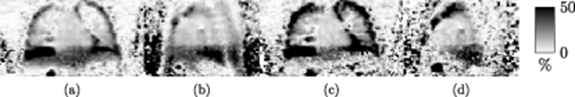
Figure 8. Patient data—Relative errors for TOF reconstruction (550 ps) in (a) coronal and (b) sagittal views and for non-TOF reconstruction in (c) coronal and (d) sagittal views.
Download figure:
Standard image High-resolution image
Additionally, spherical ROIs were drawn on the end-expiration CT for measurements using ITK-SNAP (Yushkevich et al 2006): Ascending Aorta (AA, 1.76 cm3), upper Descending Aorta (U-DA, 1.76 cm3), lower Descending Aorta (L-DA, 1.76 cm3), Left Ventricle (LV, 1.76 cm3), Right Ventricle (RV, 1.54 cm3) and Liver (7.33 cm3).
The relative differences  in different ROIs
  between
  and
and  are shown in table 3.
Table 3. Patient data—Relative errors  in TOF and non-TOF in different ROIs
  : ascending aorta (AA), upper descending aorta (U-DA), upper descending aorta (L-DA), left ventricle (LV), right ventricle (RV) and liver.
| TOF | 5.1% | 2.1% | 14.0% | 8.2% | 5.7% | 8.6% |
| non-TOF | 2.7% | 0.5% | 13.5% | 2.8% | 3.6% | 5.1% |
4. Discussion
System model inconsistencies in PET reconstruction are a cause of quantification errors. When improving the TOF resolution, local errors in the attenuation map will lead to non-local quantitative errors in the reconstructed activity image. Moreover, the errors in areas away from the attenuation mismatch increase with improved timing resolution. The errors depend on the optimisation chosen to reconstruct the data. Here we focused on MLEM/OSEM reconstructions, which are the most widely used algorithms in the clinics. We first derived a simple formula for the relative error for perfect time resolution. This formula was confirmed with simulations, by observing the trend for improved time resolution.
Results were first shown for a simple cylindrical simulation, to demonstrate the non-local effect with highly symmetrical structures. They were in agreement with Ahn et al (2014) at the centre of the mismatch, however we observed errors in areas outside of the mismatch, as predicted by the theory presented in this paper. The region in closest proximity to the mismatch (12.8 mm off-centre) presented a mixed effect: the corresponding relative error curve (figure 4) is not monotonic and resembles the curve for the ROI in the region of the mismatch at low time resolution. The study was then extended to XCAT simulations with activity at end-inspiration, first using an aligned µ map with incorrect values in the lung, and then a mismatched end-expiration µ map. As expected, the quantitative errors decreased in the lungs but increased in the neighbouring regions, such as the ventricles and the aorta. Finally patient PET data were gated (end-expiration) and reconstructed using two different µ maps: one close to the PET gate and the second one corresponding to end-inhalation. Both TOF (FWHM: 550 ps) and non-TOF were employed. The differences between the two sets of images were similar to those observed with the second XCAT simulation. While differences in the lung reduced with increased TOF timing resolution, they increased in most neighbouring ROIs, such as the ascending aorta (from 2.7% to 5.1%) or the left ventricles (from 2.8% to 8.2%), similarly to the 12.8 mm off-centre ROI of the cylindrical simulation.
The findings have clinical implications for PET in the thorax. The observed effects are likely to be most important for TOF PET/MR, where existing methods to compute the attenuation map from MR acquisitions are not quantitatively accurate in the thorax, although progress has been made to overcome this issue (Lillington et al 2019). It is likely that the problem would be largest in the case where the bones are not inserted in the MR-derived attenuation map used for the reconstruction. Effects due to errors in the attenuation map are also important for PET/CT as perfect alignment between PET and CT is usually impossible (especially in the thorax).
These results also show a possible impact on kinetic modelling. As previously stated, larger errors will be expected in regions commonly used to estimate image-derived input functions, such as the aorta or the left ventricle. From the values in tables 2 and 3, we suggest to use an input function derived from either the ascending aorta or an upper region of the descending aorta. A further complication is that errors due to attenuation mismatch depend on the surrounding activity distribution. This was reported in non-TOF PET (Thielemans et al 2008, Holman et al 2016, Merida et al 2017) but is also the case with TOF, although this dependency disappears at perfect TOF resolution (see equation (12)). As the activity distribution is globally changing over the duration of the dynamic PET acquisitions, we expect time-dependent errors in presence of an attenuation mismatch on both image-derived input function and reconstructed activity, which would affect estimated kinetic parameters. Kotasidis et al (2016) already discussed such errors and found that although the biases were reduced with improved time resolution, they could not completely be resolved.
Furthermore, as shown in figure 5 the observed effect has consequences for MCIR, where it would therefore be necessary to model the density changes in the lung Cuplov et al (2018), Emond et al (2019) in order to avoid intra-gate inconsistencies.
A possible way to correct the attenuation maps is by using an algorithm such as Maximum-Likelihood reconstruction of Activity and Attenuation (MLAA) Nuyts et al (1999). When TOF information is available, it is possible to determine, from the prompts only, the corrected attenuation sinogram up to a constant Defrise et al (2012). It becomes therefore possible to compute the entire attenuation sinogram when at least a part of it is known precisely (e.g. when a suitable region of the µ map is known). Rezaei et al (2019) has recently demonstrated clinical feasibility of MLAA, when robust calibration and corrections are used. The results in this paper imply that MLAA will become essential at higher TOF timing resolution. The effect observed in this paper also provides an alternative explanation for the fact that MLAA becomes more stable with improved TOF resolution: the non-locality of the error can be a reflection of the inconsistencies between the data and the system model if the wrong attenuation map is used (equation (8)).
This publication only focused on system model inconsistency linked to the attenuation map. The study could be extended to inconsistencies due to incorrect background term within the reconstruction (i.e. including estimation of randoms and scatters). An accurate estimation of the scatter sinogram was indeed shown to be of great importance to obtain quantitative measures in TOF-MLAA Rezaei et al (2019).
5. Conclusion
We have shown that the effect of using an incorrect attenuation map in the reconstruction on the activity image cannot be considered local in TOF reconstructions. The relative errors can be easily quantified for perfect time resolution, which should be very similar to high resolution reconstruction such as 100 ps or better.
In conclusion, even at high time resolution, using an accurate attenuation map within the PET reconstruction is essential to obtain robust quantitative measures. When the attenuation map is not known precisely enough (as is usually the case for lung imaging), the attenuation images would need to be systematically re-estimated, for example via MLAA. This is especially important in future scanners with sub-100 ps time resolution.
Acknowledgment
The authors acknowledge funding support from GlaxoSmithKline (BIDS3000030921) and research support from the National Institute for Health Research, University College London Hospitals Biomedical Research Centre.
We would also like to thank Robert Shortman for research governance and administration.
Finally, we would like to thank Michel Defrise (Department of Nuclear Medicine, Vrije Universiteit Brussel, B-1090 Brussels, Belgium) and Johan Nuyts (Department of Nuclear Medicine, Katholieke Universiteit Leuven, Belgium) for the insightful and stimulating discussion.
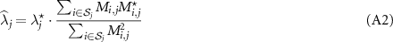
: Appendix A. Extension to other reconstruction algorithms
The notations in this appendix follows the one used in section 2.3. In this appendix, we derive formulas similar to equation (12) for unweighted least-squares reconstructions. When using pre-corrected data, this derivation is equivalent to that of filtered back-projection. The unweighted least-squares solution is obtained by solving

The solutions of (A1) with  and
and  are respectively

where ![$\left[\,\cdot\,\right]^\mathrm{T}$](https://content.cld.iop.org/journals/0031-9155/65/8/085009/revision2/pmbab7a6fieqn137.gif) is the transpose matrix operator. For a voxel pair
is the transpose matrix operator. For a voxel pair  and using (9), we have the following element of
  :
:
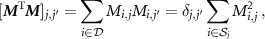
where  is the Kronecker delta. Thus,
  is a diagonal matrix and the solution
  corresponding to a given system matrix
  is therefore straightforward (provided that
  ):
):
In the noiseless situation  , then