
Abstract
In proton therapy, patients benefit from the precise deposition of the dose in the tumor volume due to the interaction of charged particles with matter. Currently, the determination of the beam range in the patient's body during the treatment is not a clinical standard. This lack causes broad safety margins around the tumor, which limits the potential of proton therapy. To overcome this obstacle, different methods are under investigation aiming at the verification of the proton range in real time during the irradiation. One approach is the prompt gamma-ray timing (PGT) method, where the range of the primary protons is derived from time-resolved profiles (PGT spectra) of promptly emitted gamma rays, which are produced along the particle track in tissue. After verifying this novel technique in an experimental environment but far away from treatment conditions, the translation of PGT into clinical practice is intended. Therefore, new hardware was extensively tested and characterized using short irradiation times of 70 ms and clinical beam currents of 2 nA. Experiments were carried out in the treatment room of the University Proton Therapy Dresden. A pencil beam scanning plan was delivered to a target without and with cylindrical air cavities of down to 5 mm thickness. The range shifts of the proton beam induced due to the material variation could be identified from the corresponding PGT spectra, comprising events collected during the delivery of a whole energy layer. Additionally, an assignment of the PGT data to the individual pencil beam spots allowed a spot-wise analysis of the variation of the PGT distribution mean and width, corresponding to range shifts produced by the different air cavities. Furthermore, the paper presents a comprehensive software framework which standardizes future PGT analysis methods and correction algorithms for technical limitations that have been encountered in the presented experiments.
Export citation and abstract BibTeX RIS

Original content from this work may be used under the terms of the Creative Commons Attribution 3.0 licence. Any further distribution of this work must maintain attribution to the author(s) and the title of the work, journal citation and DOI.
1. Introduction
Particle therapy is a widely accepted, promising option for tumor treatments, complementing conventional radiotherapy performed with megavolt (MV) x-rays and electrons. About 90 clinical particle-therapy facilities are in operation worldwide (PTCOG 2019). The well-defined range of protons or carbon ions, with a dose maximum (Bragg peak) close to the end of their trajectory followed by a sharp distal fall-off allows focusing the dose in the tumor while minimizing the damage of surrounding normal tissue. The accuracy of the expected proton range in tissue is, however, affected by uncertainties in converting CT images into particle stopping-power maps, by anatomical changes between planning and treatment, and by other factors that are hard to assess with the necessary precision in clinical routine (Harald 2012, Loeffler and Durante 2013). These uncertainties lead to rather large safety margins in the treatment planning and constrain potential benefits of particle over conventional therapies (Knopf et al 2009). In this context, considerable efforts have been made in the last two decades to develop clinically applicable methods and instruments for measuring the particle range and the dose profile in situ during treatments with millimeter accuracy (Knopf and Lomax 2013, Parodi 2016).
Particle-therapy positron emission tomography (PT-PET) is so far the only proven technique of in vivo range assessment that has been applied in comprehensive patient studies with carbon beams (Enghardt et al 2004). Efforts are ongoing to establish this technique in proton therapy as well (Lopes et al 2016).
Range verification utilizing the signature of prompt gamma (PG) rays is a promising alternative. PG radiation is produced along the beam path in nuclear reactions between the primary particles and atomic nuclei of the tissue. Its spatial emission distribution correlates well with the dose deposition map of the incident ions (Min et al 2006, Janssen et al 2014). Prompt gamma-ray imaging (PGI) can thus be used to reconstruct the range of particle beams in matter. PG cameras with passive collimation using a pin-hole (Seo et al 2006), a single slit (Smeets et al 2012), or multiple slits (Pinto et al 2014), have been investigated. So far, only the knife-edge slit camera (Smeets et al 2012, Perali et al 2014) developed by IBA (Ion Beam Applications, Louvain-la-Neuve, Belgium) has been clinically applied for PG based range verification (Richter et al 2016, Xie et al 2017). This camera is capable of detecting local range shifts of about 2 mm (Nenoff et al 2017). However, the heavy collimator may interfere with the patient and makes integration in a treatment facility challenging. An alternative approach, the Compton imaging (Everett et al 1977), was used by several groups which tried to tackle the associated challenges in the PG domain (Hueso-González et al 2014, Thirolf et al 2014, Krimmer et al 2015, McCleskey et al 2015, Llosá et al 2016). Despite encouraging results published recently (Draeger et al 2018), intrinsic hurdles like technical complexity, electronic expense, low overall efficiency, the intense flux of PG rays and the corresponding detector load to be handled, high radiation background, and the elevated percentage of random coincidences challenge the applicability of this technique, especially under consideration of therapy conditions (Golnik et al 2016, Hueso-González et al 2016, Hueso-González et al 2017, Pausch et al 2018).
Compared to Compton imaging, recent approaches using monolithic detectors instead of multi-stage arrays seem more promising and less expensive. Prompt gamma-ray spectroscopy (PGS) (Verburg and Seco 2014) analyzes intensity ratios of characteristic PG peaks measured with collimated detectors of adequate energy resolution. The nuclear reaction channels associated with relevant gamma-ray lines are distinguished by cross-sections with characteristic energy dependencies. Therefore, line intensity ratios measure the actual beam energy at the point of observation, or the residual range of the particles at the depth the collimated detector is looking at. Prompt gamma-ray timing (PGT) (Golnik et al 2014) is an alternative approach, based on the determination of the proton transit time within tissue. It is indirectly derived from the time distribution of the emitted PG rays generated by a bunched particle beam and measured with an uncollimated scintillation detector with respect to a bunch timing reference signal. Width and centroid of the PG timing peak are a function of the transit time of the particles in tissue, which is correlated with the particle range. Prompt gamma-ray peak integration (PGPI) determines the Bragg-peak position from PG count rate ratios measured with multiple detectors arranged around the target (Krimmer et al 2017). All these methods rely on relatively simple measurements that can, in principle, be performed with single scintillation detectors of reasonable energy or time resolution.
A common and crucial problem of all PG based approaches is obtaining the necessary number of events to verify the range with the reasonable precision of a few millimeters, especially in Pencil Beam Scanning (PBS) mode—the most advanced beam delivery technique (Pausch et al 2018). In PBS, the tumor is scanned in three dimensions with a particle beam focused to about the diameter of a pencil from 0.5 cm to 1.5 cm (FWHM). Lateral beam deflection by dipole magnets provides two scanning dimensions; the third one is due to the variation of the beam energy and consequently of the penetration depth (proton beam range). In a typical clinical treatment field, single PBS spots comprise up to about 108 protons (Smeets et al 2012) that are delivered in less than 10 ms (Pausch et al 2016, 2018). With a PG production rate of ∼0.1 per proton (Smeets et al 2012), around 109 gamma rays per second are emitted in 4 during beam delivery, which causes an enormous detector load. However, the time available for the range measurement is equal to the spot delivery time of a few milliseconds. Consequently, the number of measured PG events is basically determined by the achievable system throughput per detector times the number of detection units and spot duration. The detector load can be adapted by varying the detector size or the distance to the target.
After having explored the novel PGT technique (Golnik et al 2014) in first proof-of-principle experiments at clinical proton therapy facilities but far off treatment conditions (Hueso-González et al 2015, Petzoldt et al 2016), a clinically applicable hardware solution for energy and timing spectroscopy of PG rays at high throughput rates was developed (Pausch et al 2016). This work reports on the next step towards clinical application of the PGT method with the newly developed detection system. An experiment was performed in the gantry treatment room of the University Proton Therapy Dresden (UPTD) to answer two basic questions:
- (i)Is it possible to detect few-millimeter range deviations of individual proton pencil beams under clinical beam conditions by means of PGT using detection units as described in Pausch et al (2016)?
- (ii)What are the uncertainty limits, and what are the factors defining these limitations?
To answer these, an elementary experimental setup was designed. Range shifts were induced by inserting air cavities of defined thicknesses in a homogeneous polymethyl methacrylate (PMMA) target. A PGT detection unit as described in Pausch et al (2016) was used to collect data at high throughput rates for a series of single pencil beam spots. The time-resolved profiles (PGT spectra) of the promptly emitted gamma rays were acquired during the irradiation of the phantom. The data corresponding to range shifts with different cavities were compared with the reference spectra (taken without an air cavity). Such difference measurements prevent most of the systematic uncertainty introduced by modeling. At the same time, these measurements represent practical hardware tests disclosing strengths and weak points of the PGT detection system and method. Another aspect of this paper is the discussion of appropriate data analysis procedures including corrections for detector instabilities, electronic nonlinearities, background, and other effects. The software framework developed here will be used in forthcoming experiments.
2. Material and methods
2.1. Accelerator operation and beam delivery
The examination of the PGT method was performed at the University Proton Therapy Dresden (UPTD), a proton treatment facility comprising a Cyclone®230 (C230) isochronous cyclotron by IBA. The system was operated in PBS mode, where the dose is delivered in single spots to the target volume. The planned spot strength (delivered number of protons per spot) is system-internally encoded in so-called monitor units (MU). MU are a measure of the charge in an ionization chamber during the irradiation and are therefore proportional to the delivered numbers of protons. This device-specific calibration factor depends on the requested energy of the primary protons and the type of the built-in ionization chamber. In a real treatment, all information about beam delivery, as MU number, number of layers/spots, energy of layer, spot positions, spot weights are defined in the treatment plan. The treatment plan used in the experiment contains 100 equally weighted spots with a fixed proton energy (set to either 162.0 MeV or 226.7 MeV), which are all delivered to the center of the phantom (fixed position). Internally, the beam delivery system links the 100 spots to a single energy layer in the treatment plan. In the following, the term layer is used when the data are accumulated over the full irradiation time, so that the 100 single spots are considered. This plan is not intended for a realistic tumor irradiation, but its internal structure is similar to a realistic treatment plan. The main parameters of the two plans are summarized in table 1.
Table 1. PBS treatment plan parameters including the number of delivered spots  , the number of energy layers
  , the total number of monitor units
  , the number of protons per spot
  /spot, the incident beam current
  and the proton energy
  .
.
| Area |  |
 |
 |
 /spot /spot |
 /nA /nA |
 / MeV / MeV |
|---|---|---|---|---|---|---|
| Central | 100 | 1 | 1000 |  |
2 | 162.0 |
| Central | 100 | 1 | 1000 |  |
2 | 226.7 |
The selected energies result in proton penetration depths R (continuous-slowing-down approximation (CSDA)) in water of (18.04  0.05) cm and (32.15
  0.05) cm (Berger 2015). The smaller depth at 162.0 MeV resembles a clinically relevant case, while the high energy of 226.7 MeV is additionally ideal to test the capabilities of the PGT system. On the one hand, the smaller proton bunch time spread at higher energies (Petzoldt et al 2016) leads to a maximum 'sharpness' reflected in the PGT spectra (Hueso-González et al 2015). On the other hand, it allows clarifying if PGT can, unlike other PG methods (Smeets et al 2012), properly handle the higher neutron background at this energy.
For control and safety purposes, an ionization chamber monitors the charge during the irradiation. Taking into account the energy dependency of the MUs related to the number of protons, and the machine calibration factor for the conversion of MU to measured charge in the ionization chamber QIC (1 MU = 2.22 nC), the number of protons per spot can be derived. To have a comparable measure to previous experiments as well as clinical data from other centers, the presented results are always given with reference to the number of delivered protons and not to MU. As mentioned, all spots in the treatment plan have the same strength (10 MU), which results in numbers of protons per spot of  for E
for E MeV and
  for E
for E MeV (table 1). This is close to the number of protons in the strongest beam spots of clinical treatment plans (Smeets et al 2012).
2.2. The PGT detection system and module settings
The requirements concerning detector and readout electronics used in PGT were extensively studied in preliminary experiments (Hueso-González et al 2015), which lead to the detection system shown in figure 1.
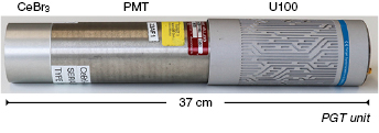
Figure 1. Photograph of the detection system consisting of a CeBr3 crystal coupled to a PMT, stacked on a U100 digital spectrometer—all together labeled as PGT unit.
Download figure:
Standard image High-resolution imageFor our experiment, we used a ø 2"  2" CeBr3 scintillation crystal, which is well suited for measuring high energy gamma radiation with an energy up to 8 MeV, while ensuring at the same time excellent timing properties. In Roemer et al (2015) the energy resolution for a CeBr3 crystal with a dimension of ø 1"
 1" was determined to be
  (FWHM) at 4.4 MeV. Additionally, the short decay time of the scintillator light of about 17 ns (Knoll 2010) allows to handle the expected high detector load in the planned experiment by minimizing pile-up.
The crystal is coupled to a Hamamatsu R13089-100 photomultiplier tube (PMT). Scintillator and PMT are housed in a common detector case with standard 14-pin PMT socket with a customized pin layout. A compact electronic unit (size: ø = 65 mm, length = 155 mm), the Target U100 spectrometer, developed specifically for this application (Pausch et al 2016), is plugged on the detector socket. It digitizes the signals with 14 bit resolution at a sampling rate equal to the system clock frequency. The U100 also comprises a software-controlled high-voltage unit with an active divider feeding the PMT dynodes with stabilized voltages, an ethernet interface for data readout, system control, and firmware updates, as well as coaxial connectors to be used for clock synchronization of multiple modules, an optional external clock reference, and optional hard-wired coincidence logics. Power is provided via the ethernet connector utilizing the power-over-ethernet (POE) standard.
The digital signal processing implemented in the U100 firmware is shared between a field programmable gate array (FPGA) and an Advanced RISC (reduced instruction set computer) Machine (ARM) processor. Every signal exceeding an adjustable threshold triggers the pulse analysis. First, the pulse charge (denoted by Q) is derived by integrating a fixed number of baseline corrected samples. Q is stored as a floating-point value normalized to the pulse charge of a signal fitting the analog to digital converter's (ADC) input range. Second, a 64 bit timestamp T is calculated. It comprises two components: (1) the coarse time  denoting the number of clock cycles elapsed since the last system start or clock reset, and (2) the fine time
  representing the pulse onset within the current system clock cycle. The latter is a 10 bit integer value provided by a timing algorithm that analyses some samples on the leading edge of the signal after baseline subtraction. The Q and T data of all valid events are streamed via ethernet to the data acquisition computer (DAQ-PC). The fixed dead time of about 1
  s per event, defined by the signal processing algorithm, determines the maximum (asymptotic) throughput rate to about 1 Mcps. The U100 unit is controlled and monitored either with a common web browser addressing the web server contained in the U100 firmware, or by using the application programming interface (API) documented in the U100 web server.
In case of the described experiment, the 106.3 MHz signal provided by the radio frequency (RF) mother generator of the proton accelerator was used as external clock reference for the U100. The built-in phase-locked loop (PLL) doubled the reference frequency to a 212.6 MHz system clock. The U100 system clock (and consequently the pulse sampling) was thus phase-locked with the accelerating RF. It provided just two clock cycles (two pulse samples) per RF period of 9.407 ns, the latter corresponding to the time interval between proton micro-bunches. The timing of a detector signal with respect to the proton bunches is then given by the 11 least significant bits of the timestamp and is denoted as relative time ( ). The full timestamp reflects the full time elapsed since clock reset and is labeled in the following as measurement time, given in seconds.
The data acquisition was performed by user software on the DAQ-PC by using the U100 API. The PGT detection system was mostly operated at a throughput around 500 kcps. This corresponds to a dead time of 50% and a detector load of around 1 Mcps. The combination of the CeBr3 scintillation detector with PMT connected to the U100 spectrometer is labeled as PGT unit (figure 1) in the following.
As investigated in Petzoldt et al (2016), the resolution of the PG emission time distribution is mainly given by the bunch time spread  of the incoming proton bunches. This is strongly depending on the requested energy and beamline settings of the proton beam and results in minimum values of around
  = 200 ps–250 ps for the maximum beam energy.
The PGT unit was characterized with an energy resolution of  E/E = 2.5% at 2.5 MeV (sum energy of 60Co) and a time resolution of
  T = 225 ps at 4.5 MeV at the ELBE bremsstrahlung facility (Wagner et al 2005) (values given as FWHM of the respective distribution). This matches well with the required parameters mentioned previously for the detection system. An energy range of 15 MeV was set with the PMT voltage (
 V) to cover the full PG energy spectrum with some reserve.
2.3. Experimental setup
The experiment was performed in the treatment room of the UPTD, which delivers a clinical proton beam by means of an isocentric, rotating gantry. We used the PBS mode in the horizontal position (270°) of the gantry. A schematic drawing of the experimental setup is given in figure 2.

Figure 2. Schematic drawing of the experimental setup in the treatment room of the UPTD. The phantom provides the opportunity to insert air cavities at a position z with a thickness s, which generate variations of the range R of the delivered fixed energy proton beam. The detector (Det) attached to the U100 (digital spectrometer) is connected via ethernet for controlling the data acquisition (DAQ) as well as for power supply using the power-over-ethernet (POE) standard. A time discriminator (Discr.) converts the sinusoidal cyclotron RF in a logical signal, which is used as external clock synchronization (Clock Sync.) of the U100 spectrometer.
Download figure:
Standard image High-resolution imageIn the experiment, two identical homogeneous PMMA targets (C5H8O2, density:  g cm−3, length: 200 mm, diameter: 150 mm), one behind the other with a total length of 400 mm, were used. A model of the combined phantom is shown in figure 3. Each target consists of two halfs of hollow PMMA cylinders, which allow the insertion of cylindric modules of different materials (e.g. air, tissue equivalent material) with a diameter of 50 mm and a variable thickness s. The identical halves were put together and the phantom, composed of the two targets, was placed on the treatment table.
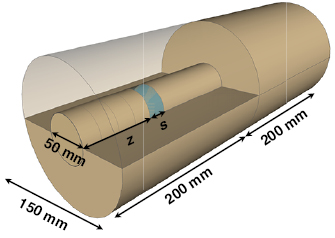
Figure 3. Phantom used in the experiment. It consists of two hollow PMMA cylinders which allow to place cylindric modules or distance rings with a diameter of ø = 50 mm and different thicknesses s at a certain depth z.
Download figure:
Standard image High-resolution imageThe PGT unit was located at an angle  of 130° with respect to the beam axis (see figure 2) at a distance of d = 60 cm. This distance represented a reasonable compromise between detector throughput and efficiency. The detector was aligned to half of the longitudinal range (R1/2) of the protons in the PMMA phantom, which is R1/2 = 140 mm for 226.7 MeV and R1/2 = 75.5 mm for 162.0 MeV (Berger 2015) (see figure 2). As the detector position was fixed, the target had to be shifted for each respective proton energy.
2.4. Measurement program and PGT analysis parameters
The treatment plan given in table 1 was delivered to the phantom (see figure 3), in which air gaps with a thickness s located at a certain depth z were introduced (see table 2). Thus, artificial range deviations of the proton beam were generated. The data analysis aims to detect relative deviations in the time resolved PG distribution with respect to a reference measurement (homogeneous PMMA target), which is recorded at the beginning or at the end of the experimental campaign. In detail, the identification of range shifts is based on the variation of the statistical momenta extracted from the measured PGT spectra of two different measurements. A detected change in the mean or the standard deviation of the PGT spectra between the related measurements serves as a measure for a proton range variation (Golnik et al 2014). The notation is chosen to be PGT mean ( ) for the first statistical moment and PGT width (
 ) for the second statistical moment. They are calculated as follows:
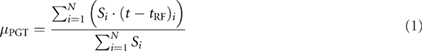

where Si denotes the content of bin i,  the center of bin i and N the total number of bins of the respective relative-time (
 ) histogram (PGT spectrum).
Table 2. Measurement program for the two energies (226.7 MeV and 162.0 MeV) at a beam current of 2 nA. The measurements are numbered in chronological order of data acquisition. The treatment plans are described in table 1.
| Energy | 226.7 MeV | 162.0 MeV | Cavity | |
|---|---|---|---|---|
| Measurement | # | # | Thickness s/mm | Depth z/mm |
| 1, 2 | 15 | 0 (reference) | 0 | |
| 3 | 11, 12, 13, 14 | 20 | 80 | |
| 4 | 10 | 10 | 90 | |
| 5, 6 | 9 | 5 | 95 | |
| 7 | 8 | 0 (reference) | 0 |
2.5. Data processing
Before the actual data analysis procedure can be performed, it is necessary to preprocess the raw data recorded during the experiment. This is organized in two separate blocks (see figure 4). The first block comprises the translation of raw data (Q, T) in to physical units (energy deposition, relative time, measurement time). Effects which have to be corrected for are drifts of the PMT gain and nonlinearities of the electronics. The results are stored as list-mode data in ROOT TTrees (Brun and Rademakers 1997). The second block generates and analyzes the PGT spectra per layer or PBS spot considering the structure of the treatment plan. The corresponding steps are explained in more detail in the following and form the software framework for PGT data processing.
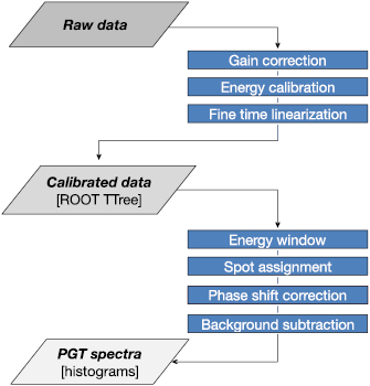
Figure 4. Overview of the correction and calibration steps, which have to be applied to the raw data. The individual steps are explained in the text.
Download figure:
Standard image High-resolution image2.5.1. Gain drift correction and energy calibration
In PBS mode, the transitions between layers with beam-on and beam-off phases lead to enormous count rate variations in the detector. In spite of stabilized dynode voltages, they cause retarded PMT gain shifts with a response time constant in the few hundred milliseconds range. This is illustrated in figure 5. The upper graphs depict count-rate histograms in a measurement-time range comprising one layer of a 226.7 MeV and a 162.0 MeV measurement, respectively. Here, 'rate' refers to the number of events actually processed per second by the U100 spectrometer (throughput). It reaches about 600 kcps or 400 kcps in beam-on phases, respectively, while the much lower rate remaining in beam-off phases is due to target activation and is dominated by 511 keV positron annihilation radiation. The lower graphs show the corresponding time evaluation of measured pulse-charge spectra in a range around the 511 keV peak. The prominent ridge in these plots represents the 511 keV full-absorption events. Its bends disclose gain shifts in the 10% range following the load leaps with some retardation. A time-dependent relationship between pulse charge and energy deposition is observed.
Figure 5. Top: the variation in the count rate for beam on and beam off intervals for proton beam energies of 226.7 MeV (left) and 162.0 MeV (right). Bottom: corresponding pulse-charge-over-time histograms for beam energies mentioned previously. The black curve indicates the shift of the 511 keV peak due to gain variations. Data were taken from the measurements in table 2 / #7, #8, where a single energy layer of 100 consecutive spots was delivered. The color scale refers to the number of collected counts per pulse-charge and time bin in the 2D histogram.
Download figure:
Standard image High-resolution imageTo correctly estimate the energy deposition for each event in spite of these gain fluctuations, a gain correction for the measured pulse charge Q is introduced. First, pulse-charge histograms are generated for consecutive measurement time bins of 60 ms width. This width is smaller than the characteristic retardation time constant of the gain response to load leaps. The position  of the 511 keV peak is determined for each time bin, as indicated by the black lines in the lower panels of figure 5. This is possible since annihilation radiation is present in the beam-on as well as in the beam-off phases. Finally, the measured pulse charge Q of each event is complemented with a gain-corrected pulse charge
  .
.  is the reference peak position determined for the last time bin and
  is the peak position in the corresponding measurement time bin. The analysis software stores
  in the output ROOT TTree. This event-wise mapping ensures that further analysis steps are independent of the binning grid used for determining the gain correction.
Figure 6 presents the evaluation of calibrated energy values, derived from the corrected pulse charge data, over the measurement time for the same measurements as shown in figure 5. The plots comprise the full energy range of interest and prove stable positions of prominent gamma ray lines. A linear energy calibration was performed by using the 511 keV and 4.44 MeV full-absorption peaks as well as the zero point ( , Energy = 0). The latter can be used since the U100 firmware corrects the pulse-charge tag Q event-by-event for a pedestal due to the actual baseline shift. Calibrated PG energy spectra comprising full measurements for the two different proton energies are given in figure 7. They show the expected characteristic structures, namely prominent PG full-absorption lines, corresponding single (SE) and double escape (DE) peaks, the 2.2 MeV gamma ray line from neutron capture on hydrogen, and the 511 keV annihilation radiation peak.
Figure 6. Energy-over-time histograms for 226.7 MeV (left) and 162.0 MeV (right) beam energies. After applying the event-wise gain correction, an energy calibration based on the prominent energy peaks can be performed. Data correspond to the measurement depicted in figure 5. The color scale refers to the number of counts per energy and time bin.
Download figure:
Standard image High-resolution image
Figure 7. The calibrated PG energy spectra of a reference measurement for 226.7 MeV (black) and 162.0 MeV (blue) proton beam energies. Clearly visible is the response to the PG rays arising from the ground state transition in 16O, 11B and 12C (Smeets et al 2012). The peaks are accompanied by their respective single (SE) and double escape peaks (DE). Additional PG ray transitions from 10B, 11C and 1H(n, )2H are also visible in the low energy part. No background subtraction or time filter was applied here. The data were taken from the measurements #7, #8 in table 2. The energy window used for the PGT analysis is indicated between 3 MeV–5 MeV (see section 2.5.3).
Download figure:
Standard image High-resolution image2.5.2. Correction of differential time nonlinearities (fine time linearization)
Time measurements with analogous as well as digital pulse processing techniques exhibit differential time nonlinearities due to imperfections in the hardware or imperfect time determination algorithms. In the current spectrometer firmware, the algorithm for the determination of the pulse onset within a clock cycle is based on a linear extrapolation of the rising pulse edge to the baseline. As already mentioned, the algorithm provides the fine time  as a 10-bit integer. The linear approximation leads to a slight dependence of the estimated timing point for a given pulse with realistic (nonlinear) slope from its position relative to the ADC sampling grid, reflected in a differential nonlinearity of the timing spectrum.
The effect becomes evident, if one analyzes events which are not correlated with the ADC sampling pattern (or, in our case, with the cyclotron RF). The expected timing distribution is uniform, corresponding to a cumulative distribution function  (figure 8, left (red)):
where i denotes the respective timing channel index [1,1024] and  the expected probability of the fine time value
  . Results of a corresponding
  measurement are shown in figure 8 (upper right panel). The timing distribution was obtained from uncorrelated events registered in a beam-off period and is obviously non-uniform. The corresponding cumulative distribution function
  (figure 8, left (black)) can be constructed from the measured timing spectrum:

where  is the measured probability to measure the fine time value and ck the channel content of the measured time distribution. This nonlinearity can be corrected for, if the measured fine time value
  is replaced by a corrected value
  fulfilling the condition
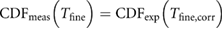
or

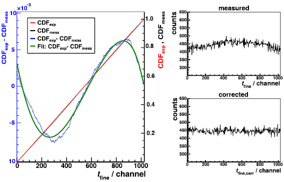
Figure 8. Due to timing nonlinearities, the fine time histogram (right/top) of events which are not correlated with the ADC sampling pattern, is not uniformly distributed. In the left panel, the measured  (black) and the expected
  (red) as well as their deviation
  –
– (blue) are shown. This deviation is fitted with a polynomial function (green) and the correction is applied event by event, which leads to the uniform distribution (bottom/right), as expected.
Download figure:
Standard image High-resolution imageThe deviation  –
– (figure 8, left (blue)) is fitted with a polynomial function (figure 8, left (green)) and the correction is then applied to all events including data taken during the beam-on periods, assuming that the differential timing nonlinearity depends on the pulse shape but not on the pulse amplitude. The analysis software includes the new event tag
  in the output ROOT TTree. The lower right panel of figure 8 proves that the correction indeed leads to a uniform time distribution of uncorrelated events.
2.5.3. Energy window
PGT spectra should ideally comprise only events due to prompt gamma-ray detections. In practice, activation and neutron-induced reactions produce an uncorrelated or delayed background, visible in the energy-over-relative-time histogram (figure 9, left) as well as in corresponding PGT spectra (i.e. corresponding projections on the ( ) axis) before (left of) or behind (right of) the prompt gamma-ray timing peak. This background can obviously be reduced by an energy window, though on the expense of statistics in the PGT spectrum (figure 9, right). Most uncorrelated events, in particular those due to gamma rays from positron annihilation and neutron capture on hydrogen, can be suppressed by considering only energy depositions above 2.2 MeV. Gamma-ray energies above 6.1 MeV are often due to neutron-induced reactions: an upper energy limit is therefore useful as well. The PGT spectra used for further analysis comprise only events distinguished by energy depositions between 3 MeV and 5 MeV. This energy window is additionally marked in the energy spectra in figure 7 and is set by means of the calibrated energy tag in the corresponding ROOT TTree.
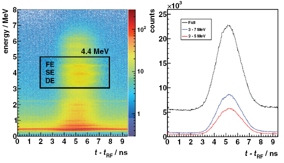
Figure 9. Left: Energy-over-relative-time spectra for a reference measurement (table 2, #15) comprising 100 spots for a proton beam energy of 162.0 MeV. The black frame indicates the considered events for subsequent data analysis (FE—full energy peak, SE—single escape peak, DE—double escape peak) from carbon and boron de-excitation. Clearly visible as a line at 2.2 MeV are uncorrelated gamma rays from neutron capture on hydrogen. Right: The corresponding relative-time spectra containing events after applying different energy windows around dominant PG peaks. This suppresses the background and improves the signal-to-background ratio but reduces the number of events in the PGT peak.
Download figure:
Standard image High-resolution image2.5.4. Spot assignment
A verification of range deviations on spot level requires the assignment of PGT data to single spots of the treatment plan. This can be done by combining knowledge about the structure of beam delivery, recorded in the PBS treatment plan and the corresponding machine log file, with an analysis of the count rate histograms.
Figure 10 shows that individual spots of a PBS plan are distinguishable due to a sharp count rate drop in the short beam-off period between two spots. The spot length depends on the beam current and the requested number of protons. Here it is, however, important to know that strong PBS spots are sometimes split in sub-spots by the beam delivery system. This happens whenever the spot charge to be delivered (measured in MU) exceeds a certain threshold. In the treatment plan applied, one PBS spot is actually delivered in three portions, each with a duration about 23 ms.
Figure 10. Count-rate-over-measurement-time histogram for a selected section between spot #29–#31 of measurement #1 in table 2. Due to the smaller bin width used here with respect to figure 5, it is possible to resolve individual spots in time by the count rate dropping down to a local minimum. One spot from the used treatment plan is internally split by the beam delivery system in three equal subspots with a length of around 23 ms, which causes the substructure. Consequently, a predefined single spot from the given plan is delivered in around 69 ms.
Download figure:
Standard image High-resolution imageKnowing this structure, the start and stop time for each individual spot can be extracted from the count rate variation as a function of the recorded timestamps. The analysis software assigns events in between these limits to the respective spots, and accumulates corresponding PGT single-spot spectra considering the energy window discussed previously.
2.5.5. Phase shift correction
As mentioned in section 2.2, the accelerator RF is used as external clock reference between the synchronized PGT unit and the proton bunch extraction. Ideally, the entrance time of the protons in the target with respect to this time reference and thus the rising edge of the PGT spectra should always stay at the same position as long as the beam energy is kept constant. However, minimal variations of the cyclotron's magnetic field (e.g. due to changing magnet temperature) slightly affect the orbital frequency of the accelerated protons and lead to a small phase mismatch per turn between proton movement and RF. With increasing number of turns, the little differences may add up to a measurable phase slip that varies in time, depending on the actual accelerator tuning. Corresponding long-term shifts of the PGT spectrum have already been observed (Petzoldt et al 2016) and can shadow range variations derived from the PGT spectrum.
As already concluded in Petzoldt et al (2016) a proton bunch monitor measuring the actual timing between RF and proton bunches could overcome this problem. Such a monitor could be based on the detection of scattered protons as proposed in Petzoldt et al (2016), or a pickup electrode measuring the beam phase directly (Timmer et al 2006). However, such a monitor has not yet been installed in the UPTD treatment beamline. Therefore, means for considering bunch-to-RF phase shifts in the PGT spectrum analysis had to be introduced. An obvious approach is to use the leading edge of the PGT spectra themselves as reference. If phase shifts occur at a time scale of minutes (Petzoldt et al 2016), the correction needs to be determined only once per measurement lasting only a few seconds (see figure 6), i.e. by using PGT spectra summed over the complete measurements. The better statistics of the summed spectra improves the accuracy of the leading-edge matching. Nevertheless, it is to state that this approach is not a means of choice for later clinical applications but only justified by the missing proton bunch monitor.
The phase shift correction is performed as follows: one of the measurements for a given beam energy is defined as reference. In the corresponding PGT spectrum R with the bin contents ri, a region of interest (ROI) is defined that comprises the leading edge of the PGT peak. The summed PGT spectrum M of a measurement to be analyzed with bin contents mi is subsequently shifted by an integer number of bins j in a reasonable range, and a set of correlation coefficients Kj is calculated in the given ROI between R and the shifted spectra:
Finally, the leading edge shift s is determined as the floating-point argument providing the maximum of a polynomial function representing the best fit of the set of points (j , Kj ).
To estimate the uncertainty of the phase-shift correction, each measured PGT spectrum M is 104 times replaced by a spectrum Mk following the same cumulative distribution function but obtained by Monte Carlo simulation considering the Poisson statistics of the distinct bin contents. For each generated spectrum Mk, the leading edge shift sk is determined and histogrammed. The standard deviation  of the Gaussian fit from the resulting sk distribution is then taken as the respective leading edge shift uncertainty
  .
.
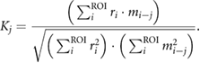
The left panel of figure 11 presents the leading edge shifts for the measurements at 226.7 MeV and 162.0 MeV proton energy, translated in picoseconds, together with an exemplary sk distribution (right) illustrating the uncertainty.
Figure 11. Left: The leading edge shift s over the number of measurements (chronological order) determined for all PGT spectra of the two proton beam energies (black: 226.7 MeV, blue: 162.0 MeV). Right: The distribution of the leading edge shifts sk obtained by Monte-Carlo simulation for the first recorded measurements (table 2 / #1, #2). The respective standard deviation  of the Gaussian fit (red) gives the uncertainty
  added to the respective data point in the left panel.
Download figure:
Standard image High-resolution imageTechnically, the phase shift correction is considered by subtracting the respective leading edge shift s (as well as a random value between 0 and 1 ps to prevent discretization effects) from the relative time tags read from the list-mode data before accumulating the respective PGT spectrum.
2.5.6. Background subtraction
When calculating the PGT mean and PGT width of the spectra, one has to consider a possible background. In spite of the energy window introduced previously, a significant amount of background remains (see figure 12). The parameters of interest for range verification given in equations (1) and (2) are therefore background corrected by using

where l and r mean the bin numbers of the left and right border of an appropriate time window comprising the PGT peak, and Bi is the background content comprised in bin i.

Figure 12. The reduced-layer (see section 3.3) PGT spectra (spot #31–#100) from protons with an energy of 226.7 MeV (left, table 2 / #1) and 162.0 MeV (right, table 2 / #15). The relative-time window set in the further analysis is marked in green. For background modeling, a linear function (red) was defined in the respective fit ranges marked with the black dotted lines.
Download figure:
Standard image High-resolution imageAs suggested by figure 12, a linear background model is used:

where  is the background pedestal and b the slope. Figure 13 shows the results of background fits performed for each single-spot PGT spectra of an exemplary measurement. The background pedestal (left) as well as the background slope (right) remains constant within the measurement and was determined to be (9.92
  0.06) counts and (1.95
  0.05)
0.05)  counts/channel as average value, respectively.
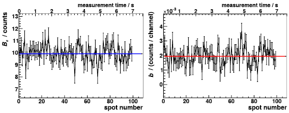
Figure 13. Background pedestal  (left) and background slope b (right) obtained from the 100 single-spot PGT spectra of a distinct measurement (table 2 / #1) by linear fits according to equation (5). The spot number (abscissa) is translated in a corresponding measurement time with respect to the start time of the first spot (second abscissa). The pedestal (
 = (9.92
  0.06) counts) as well as the slope (
 = (1.95
  0.05)
0.05)  counts/channel) stays constant within the measurement.
Download figure:
Standard image High-resolution imageFinally, the correction and calibration process results in a set of time-resolved-emission spectra—PGT spectra—for each single spot of the individual measurements, and can be used for the final analysis regarding range deviations.
3. Results
PGT spectra were generated on a full-layer and single-spot level to answer the questions posed in the introduction. The first subsection describes general features of the spectra. In the second subsection, the behavior of the PGT mean and PGT width for single-spot PGT spectra within a layer is discussed. Conclusions about the sensitivity of these parameters to range variations and on present limitations concerning minimum detectable range deviations are derived from uncertainty analysis presented in the third and fourth subsections.
3.1. General features of PGT spectra
Figure 14 shows background-subtracted, phase-shift corrected, and normalized PGT spectra of measurements without (reference) and with air cavities of different thicknesses s (see figure 3) for proton energies of 226.7 MeV (left) and 162.0 MeV (right). All histograms comprise the events of all 100 spots of the corresponding measurements and thus represent full-layer PGT spectra. The respective statistics are comparable to that of a single field from a clinical treatment plan.
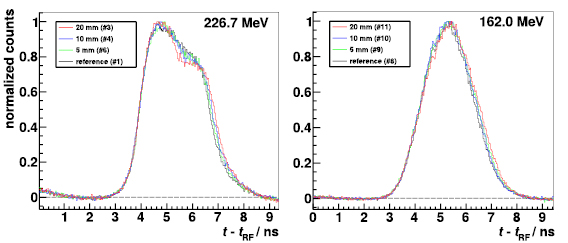
Figure 14. The PGT spectra of measurements comprising a full-layer of 100 spots (left: 226.7 MeV, right: 162.0 MeV). The black curve belongs to the homogeneous PMMA measurement which serves as reference. The different colors indicate air cavities with a thickness of 5 mm–20 mm inserted in the phantom. The distributions are shifted in time to match their leading edges as explained in section 2.5.5 and are normalized to their respective maximum.
Download figure:
Standard image High-resolution imageThe histograms corresponding to different air cavity thicknesses clearly show features as already described in Hueso-González et al (2016). At the highest available proton energy, the air cavities cause visible dips in the PGT peak indicating the reduced PG production at a certain target depth (the location of the cavity) corresponding to a certain time of PG detection. In addition, the longer range induced by the air cavity widens the PG emission time window and enlarges the time-of-flight to the detector for gamma rays produced at the end of the proton range, which shifts the trailing edge of the PGT peak to larger relative times. Such edge shifts are also visible at 162.0 MeV proton energy, but the dips disappear. This is due to the larger proton bunch width reducing the PGT resolution (Hueso-González et al 2016, Petzoldt et al 2016). Note that trailing-edge shifts are only visible if the phase-shift correction (see section 2.5.5) is applied; otherwise the PGT peak shifts, caused by an instable phase relation between proton bunch extraction and RF, would shadow this effect.
Figure 15 shows exemplary single-spot PGT spectra with and without a 20 mm air cavity corresponding to the two energies. It is evident that the low event statistics entirely hides all cavity-induced spectrum features that are nicely visible at the full-layer level. An analysis of the spectrum shape seems unfeasible. Following the idea pursued in Golnik et al (2014), further efforts have therefore been focused on a statistical analysis based on the universal PGT spectrum parameters given in equation (3) and (4) of the PGT peak derived from phase-shift and background-corrected PGT histograms.
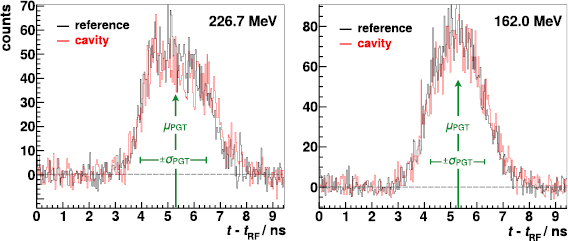
Figure 15. PGT spectra of a single spot for a proton energy of 226.7 MeV (left) and 162.0 MeV (right) from the 20 mm air cavity measurement (red) superimposed with a reference measurement (black). For a spot-wise analysis of range variations through the PGT spectra, it is necessary to determine the PGT mean ( ) and the PGT width (
 ) for each spot of the delivered PBS plan.
Download figure:
Standard image High-resolution image3.2. PGT mean and PGT width behavior within a single layer
Figure 16 shows the PGT mean and PGT width data for full sets of single spots delivered with the 226.7 MeV and 162.0 MeV PBS treatment plans of table 1 to a homogeneous (reference) and a phantom with 20 mm inserted air cavity. As all data discussed subsequently, they were computed for events with energy depositions E between 3.0 MeV and 5.0 MeV (see figure 7) and for relative-time values ( ) between 2.75 ns and 8.26 ns (time window, see figure 12), considering a phase shift correction derived for the corresponding full-layer spectrum (see section 2.5.5) as well as a spot-wise linear background subtraction (see section 2.5.6).
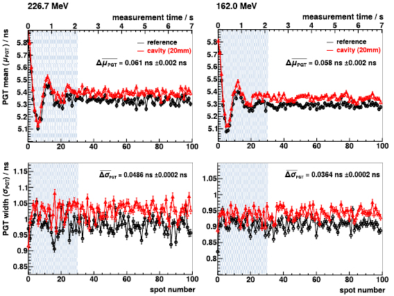
Figure 16. PGT mean (top row) and the PGT width (bottom row) extracted from the 100 spot PGT spectra for a reference measurement (black) and a 20 mm air cavity (red) for the two different proton beam energies 226.7 MeV (left) and 162.0 MeV (right). The given values  and
and  are average values for the respective deviation of spot #31–#100 (spots right from the blue shaded area). The oscillation of the PGT mean at the beginning (about the first 2 s, note the additional time axis at the top) occurs whenever the beam is switched on between the layers in the treatment plan. The PGT width is less influenced and is more robust against this effect.
Download figure:
Standard image High-resolution imageThe data exhibit the expected difference between PGT mean and PGT width for measurements with and without range extension caused by the air cavity, but also a strong and unexpected damped oscillation of the PGT mean in the first 1.5–2 s of the measurement with an amplitude exceeding the range-induced difference by about an order of magnitude. The oscillating PGT peak position obviously disturbs any range estimate based on the PGT mean. The PGT width keeps rather stable; only a slight reduction in the first spots is observed, which is obviously due to a trailing-edge cut when the PGT peak is right-shifted in the fixed time window during the first oscillation phase.
We assume that this oscillation is caused by the accelerator, namely by a swing into the full accelerating dee voltage at the beginning of each layer after a reduction in the beam-off phase between layers, which is a given feature of the IBA Proteus® PLUS operation. So far, there is no direct proof of this assumption, but there are several indications. First, different detectors behave in the same way; amplitude and period of the oscillations are not affected by changing detectors. Second, similar effects have never been observed at load-leap tests with macro-pulsed bremsstrahlung beams at the ELBE facility of Helmholtz–Zentrum Dresden–Rossendorf (HZDR) (see Pausch et al (2016)). Third, period and damping behavior of the PGT peak oscillation agree with that of tentative dee voltage logs taken during follow-up experiments.
Figure 15 implies that phase-shift corrections as determined for the full-layer PGT spectra could not be applied at spot level to eliminate the oscillations, just because of the low event statistics. A first attempt yielded uncertainties of 30 ps–40 ps or even more for determining leading edge shifts on single-spot level, which is much larger than the PGT mean shift due to a 20 mm air cavity (see figure 16). The problem could eventually be solved by an appropriate proton bunch monitor, which is, however, not yet at hand. Finally, the effect of these oscillations on the results discussed in the following could only be eliminated by excluding the first 30 spots of every layer from further analyses.
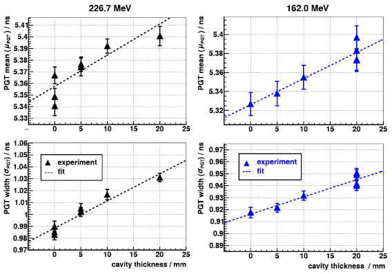
3.3. PGT mean and PGT width sensitivity to range variations
Following this insight, PGT spectra were computed for all measurements listed in table 2 by summing up the spot-level histograms corresponding to spots #31–#100 of each layer (i.e. measurement), respectively. The parameters  and
and  were then derived from these reduced full-layer spectra. Figure 17 illustrates the dependence of these parameters on the cavity thickness and thus on the excess range of the proton beam due to these cavities for proton energies of 226.7 MeV and 162.0 MeV. The error bars denote the measurement uncertainties, which are discussed in more detail in the following.
Figure 17. The statistical parameters (top: PGT mean, bottom: PGT width) of the PGT spectra are sensitive to the penetration depth of the primary protons. With increasing air gap (larger range in the target), the distribution becomes broader, which leads to an increasing PGT width and at the same time to a shift of the PGT mean to higher relative-time values. The experimental data points are extracted from the summed PGT spot spectra (spot #31–#100) of the respective measurements (table 2) after applying the discussed correction and processing algorithms (some cavities were measured multiple times).
Download figure:
Standard image High-resolution image
As expected, the distribution becomes broader with an extended cavity thickness or longer proton beam range, which leads to an increased PGT width and to a shift of the PGT mean to higher relative times. The linear fits (dotted lines) describe the correlation between spectrum parameters and cavity thickness quite well, within the uncertainty limits. The slopes of these fits are given in table 3. They describe the sensitivity of the statistical parameters to range variations and allow estimates of the range uncertainties that could be achieved by using PGT for range verification. We observed PGT mean shifts of 2.7 ps mm−1 to 2.8 ps mm−1 for both energies and a PGT width increasing by about 1.4 ps mm−1 or 2.2 ps mm−1 for the lower and the higher beam energy, respectively. These numbers illustrate the accuracy of timing required for PGT-based range verification: Timing shifts (e.g. due to time drifts or oscillations between the proton bunch and timing reference signal, or due to load effects changing the detector timing) and variations of the system time resolution (e.g. due to changing detector properties or a variation of the proton bunch width) must not exceed 2 ps–4 ps if the range should be monitored with 1 mm–2 mm precision.
Table 3. Sensitivity of PGT mean and PGT width on the excess range of the proton beam caused by air cavities inserted in the phantom. The slope parameters were obtained from linear fits of PGT data measured with air cavities of 0–20 mm thickness (see figure 17).
| Beam energy | Slope / (ps cm−1) | Beam energy | Slope / (ps cm−1) | ||
|---|---|---|---|---|---|
| 162.0 MeV |  |
27.6  0.6 0.6 |
226.7 MeV |  |
26.8  0.4 0.4 |
 |
14.4  0.2 0.2 |
 |
22.8  0.2 0.2 |
||
3.4. Uncertainty limits of PGT-based range verification
An estimate of uncertainty limits for PGT-based range verification according to the present state-of-the-art must be based on an analysis of systematic and statistical uncertainty contributions to the PGT mean and PGT width parameters. Therefore, these uncertainty contributions have to be discussed in more detail.
Tables 4 and 5 summarize the uncertainty contributions  and
and  to
to  and
and  for the two proton energies. The results were derived from the reduced-layer PGT spectra (70 spots) according to table 1 for all single measurements (table 2), and the respective average uncertainty contributions were listed in the tables. With the sensitivity (slope parameters, table 3) derived in the previous section, their contributions can be translated in corresponding range uncertainties, denoted as
 .
.
Table 4. Average uncertainties of the statistical parameters shown in figure 17 (left) for a proton beam energy of 226.7 MeV.
| Uncertainty contributions | ||||
|---|---|---|---|---|
| Source |  / ps / ps |
 / ps / ps |
 / mm / mm |
 / mm / mm |
| Phase shift correction | 6.4 | 1.4 | 2.4 | 0.6 |
| Gain correction | 2.1 | 0.8 | 0.8 | 0.4 |
| Counting statistic | 3.1 | 2.6 | 1.2 | 1.1 |
| Total | 7.4 | 3.1 | 2.8 | 1.3 |
Table 5. Average uncertainties of the statistical parameters shown in figure 17 (right) for a proton beam energy of 162.0 MeV.
| Uncertainty contributions | ||||
|---|---|---|---|---|
| Source |  / ps / ps |
 / ps / ps |
 / mm / mm |
 / mm / mm |
| Phase shift correction | 11.9 | 2.1 | 4.3 | 1.5 |
| Gain correction | 0.4 | 0.4 | 0.1 | 0.3 |
| Counting statistic | 2.7 | 2.4 | 1.0 | 1.7 |
| Total | 12.2 | 3.2 | 4.4 | 2.3 |
A first contribution arises from the phase shift correction. The correction procedure as well as the method to determine its uncertainty is described in section 2.5.5. The contributions given in tables 4 and 5 represent the square root of the variance of the respective leading edge shift distributions as illustrated in figure 11 (right panel).
The second contribution is due to detector gain variations that are not fully compensated by the gain drift correction (section 2.5.1). Remaining gain deviations lead to an incorrect energy calibration and actually result in event selection based on a shifted energy window. This might affect the shape of PGT spectra. To estimate the maximum uncertainty, the complete analyses were repeated with energy windows corresponding to gain drifts of  2% in case of 226.7 MeV and
  0.5% in case of 162.0 MeV proton energies, and the resulting PGT mean and width variations were assumed to represent maximum uncertainty contributions. These gain drifts correspond just to the maximum dynamic gain change within a 60 ms time bin as used for computing the gain drift correction. The larger gain drift at the higher proton energy is due to the sharper and stronger gain jump after starting dose delivery (see figure 5).
The third contribution results from the limited PGT spectrum statistics. On the one hand, the accuracy of determining the respective parameter (PGT mean, PGT width) depends of course on the number of collected events per PGT spectrum. On the other hand, the limited statistics in the PGT spectrum leads to an uncertainty of the estimated background underlying the PGT peak. Therefore, the resulting statistical uncertainty using the suggested linear background model (section 2.5.6) has to be determined.
For estimating the mentioned statistical contributions, a similar procedure as for the phase-shift correction was used. The respective measured PGT spectra were re-generated 104 times (104 iteration steps j ) by randomizing the content of each bin assuming a Poisson distribution around the original bin content Si. The number of entries in each generated PGT spectrum is constant and given by the number of entries of the measured PGT spectrum. The background contribution was individually fitted for each re-generated PGT spectrum. For every iteration j ,  and
and  were determined and histogrammed. The widths (square root of variances) of the two corresponding distributions were given as statistical uncertainties in the last row of table 5. They depend, of course, on the PGT spectrum statistics. Table 6 compares therefore different cases. First, data for the reduced-layer and single-spot PGT spectra as measured in our experiment are given, together with the corresponding number of protons delivered to the target. The second block comprises data derived for proton numbers of typical strong PBS spots in real treatments (Smeets 2012, Pausch et al 2018). They are discussed in more detail in the following. This table is restricted to data for 162.0 MeV proton energy, since this is a more clinically realistic and also more critical case. The error bars in figure 17 illustrate the root sum squared of systematic and statistical uncertainties for the analyzed reduced-layer PGT spectra. It is evident that the largest uncertainty contribution is due to the phase-shift correction. However, for single spots, the statistical component becomes dominating.
Table 6. Statistical uncertainties of PGT-based range verification at 162.0 MeV proton beam energy considering a different number of delivered protons  .
.
| Statistical uncertainty contributions | |||||
|---|---|---|---|---|---|
 |
Description |  / ps / ps |
 / ps / ps |
 / mm / mm |
 / mm / mm |
2.7  |
Experiment / layer | 2.7 | 2.4 | 1.0 | 1.7 |
3.8  |
Experiment / spot | 28.5 | 20.1 | 10.3 | 14.0 |
1.0  |
PBS spot | 44.2 | 39.7 | 16.0 | 27.6 |
8.0  |
PBS spot (eight detectors) | 15.7 | 14.4 | 5.7 | 9.9 |
3.2  |
PBS spot, aggregation, eight detectors | 7.5 | 7.1 | 2.7 | 4.9 |
4. Discussion and conclusion
Currently, we focus on a clinical implementation of the PGT method, which requires an evaluation under treatment conditions. Therefore, methods and concepts in PGT analysis gained from previous proof-of-principle experiments were transferred, tested and expanded based on the experimental data recorded under close-to-clinical beam conditions.
In the course of the analysis, a comprehensive software framework was developed to improve the PGT data processing and analysis procedure with special focus on future clinical applications. This includes a standardized procedure for the stabilization of the PMT gain, the energy calibration and time nonlinearity corrections. The detected variation in the gain due to the enormous load variation could be compensated via an event-wise correction. Regarding a clinical PBS plan comprising various layers with different proton energies, this correction is mandatory for a robust energy calibration. In the resulting calibrated energy spectra, the dominant PG lines are clearly visible, which allows a definition of fixed energy windows around the prominent peaks. These energy windows are convenient to suppress the background.
The time nonlinearities were corrected event-by-event. Here, the current analysis indicates that the individual correction functions of the different measurements are stable over the measurement campaign. Therefore, the correction algorithm could be further simplified by using a global look-up table derived from a representative measurement for the whole measurement campaign.
The common background suppression in the PGT analysis using an energy window around the prominent PG peaks and a relative-time window in the PGT spectra was extended by subtracting the background underlying the PGT peak. Therefore, a linear fit function was modeled to the background for each single-spot PGT spectrum. This procedure will be routinely used in future analysis, where the offset of the modeling function has to consider the growing radiation background from activation while the slope can be assumed as constant within a layer.
Additionally, a sorting algorithm was developed, which allows a spot-wise assignment of the correlated PGT spectra. This is especially important for future applications with clinical treatment plans delivered to complex volumes. This enables a local determination of range deviations for single spots.
The problem of the proton bunch phase drifts, already known from previous experiments, is due to the unstable phase correlation between the accelerator RF and the proton bunches. As explained in section 2.2, the RF serves as reference signal for the PGT measurements which means that the PGT spectra and, in particular, the associated statistical momenta of the distributions are directly influenced by these instabilities. The phase drifts cause a shift in the leading edges of the PGT spectra, which is directly translated into a shift of the PGT mean. This variation in the PGT mean can be falsely considered as a range deviation of the proton beam and must be corrected for. In the presented experiment, these drifts were determined to be in the range of a few tens of picoseconds and could be analytically corrected for the full-layer PGT spectra with respect to a reference measurement.
In addition, an effect appeared which causes a damped oscillation of the absolute PGT mean among the 100 PGT spot spectra within a measurement. The shift of the PGT mean is in the range of a few hundred picoseconds for the first spots in a measurement, which are delivered in around 2 s. It seems that this oscillation is accelerator specific and could vary between the treatment fractions. A first application of the PGT method in a real patient treatment requires solving this issue. However, the PGT width is more robust against this effect.
The values of the phase drifts and phase oscillations are orders of magnitudes higher than the actual observable. This underlines the urgent need of a proton bunch monitor as proposed by Petzoldt et al (2016). The requirements of such a system can now be more accurately defined. It should be able to monitor the bunch-RF phase drifts at a time scale of minutes as well as the phase oscillations occuring within 1–2 seconds with an accuracy of around 2–3 ps.
Despite all these constraints, the measured and corrected PGT spectra show the expected results. The dependency of the statistical momenta ( ,
,  ) from inserted air cavities with variable thicknesses could be quantified. After setting an energy and timing window, applying the background subtraction and correcting for the phase drifts, as well as excluding the first 30 spots due to the oscillation, the PGT mean and PGT width were determined in the PGT spectra for the different measurements. The variation of the statistical momenta depending on the thickness of an inserted air cavity in a PMMA phantom was predicted for a 150 MeV proton beam in Golnik et al (2014), with
  = 40 ps cm−1 and
  = 18 ps cm−1. The presented experimental values (table 3) for the standard deviation are in good agreement, whereas the mean is higher in the simulation.
Based on the uncertainty estimates (tables 4–6) and the sensitivity of the slope parameters (table 3) derived from the experimental data, it is now possible to identify key problems for translating PGT to the clinics and to assess the achievable accuracy of range verification. As a matter of fact, the limited event statistics proves being the major problem. According to table 3, the statistical uncertainty contributions of 44 ps or 40 ps (PGT mean and width, respectively) in case of a PGT spectrum measured with a single detector for a single strong PBS spot in a treatment translate to range uncertainties of 16 mm–28 mm. An obvious idea is using multiple PGT detectors, but even with eight detectors it is not possible to reach range accuracies below 6 mm–10 mm. An additional spot aggregation as applied with other instruments (Smeets et al 2012, Richter et al 2016, Nenoff et al 2017), here assumed to provide a factor of four in the event statistics, or a corresponding improvement in the spectrometer's throughput, lead to a range verification with 3 mm precision (last line in table 6), supposed the systematic uncertainties could be reduced noticeably as well. Looking at the latter, the phase shift correction generates the largest uncertainty. As discussed previously, a proton bunch monitor (with a pickup electrode (Timmer et al 2006), prompt-gamma-ray detector close to the degrader, proton monitor detecting off-scattered protons, or similar) should tackle this problem. To finally achieve a precision of 1–2 mm, a further improvement of the statistic is obviously necessary. This could be achieved by improving the throughput per detector and by further increasing the number of detectors, e.g. by using arrays of smaller pixels instead of monolithic detectors (Pausch et al 2018). The collimator-free construction and the favorable detector arrangement around the treatment snout, which prevents any interference with the beam or the patient couch, are good arguments to continue with corresponding research.
The presented results encourage further experiments in more realistic clinical conditions. Namely, the irradiation of complex volumes using multiple layers and spots of variable weight, which causes a variable number of incoming protons per spot and layer. For these future experiments, the developed software framework ensures a standardized analysis and increases the reproducibility.
Acknowledgements
The authors would like to thank the local IBA team for their very kind support and for the stable operations.