
Abstract
This paper addresses unresolved issues related to the safety of persons with conductive medical implants exposed to electromagnetic (EM) fields. When exposed to EM fields compatible with the reference limits—in particular <100 MHz—implants may enhance local fields and energy absorption to values much higher than the basic restrictions that are considered safe. A mechanistic model based on transfer functions has been postulated for elongated active implants at magnetic resonance imaging (MRI) frequencies and used as a basis for standards dealing with MRI implant safety. However, this mechanistic model is inconsistent with the behavior observed for electrically short implants, such as abandoned leads in MRI or active implants under low-frequency exposure conditions (e.g. wireless power transfer). In this paper, a new mechanistic model for electrically short implants is proposed that allows implant safety assessment to be decomposed into separate steps. Per tip-shape, it requires only a single simulation or measurement of the implant exposed under (semi-)homogeneous conditions. To validate the approach, predictions of the mechanistic model were compared to results of numerical simulations for electric- and magnetic-field exposures. The impact of parameters such as tissue properties, length, tip shape, and insulation thickness on safety- and compliance-relevant quantities was studied. Validation involving an anatomically detailed computational human body model with a realistic implant at multiple locations under electric and magnetic exposures resulted in prediction agreement on the order of 7% (maximal deviation <15%). The approach was found to be applicable for electrical lengths up to 20% of the effective wavelength and can be used to derive suitable testing procedures as well as to develop safety guidelines and standards.
Export citation and abstract BibTeX RIS

Original content from this work may be used under the terms of the Creative Commons Attribution 3.0 licence. Any further distribution of this work must maintain attribution to the author(s) and the title of the work, journal citation and DOI.
1. Introduction
1.1. Exposure safety concerns for persons with medical implants
The presence of a conductive medical implant—where the electrical conductivity of the implant ( ) is much greater than that of the surrounding tissues (
 )—can result in large localized field enhancements in the human body (Kyriakou et al 2012) that are not consistent with current safety guidelines (ICNIRP 1998, 2010, IEEE C95.1 2005). This means that the basic restrictions are exceeded even for exposure values that are below the reference limits. As the enhancement may be two orders of magnitude or more (Kyriakou et al 2012), this constitutes a potential safety hazard due to induced tissue heating (Kyriakou et al 2012, Awal et al 2015) at frequencies ⩾100 kHz or through interference with nerve or organ electrophysiology (Reilly et al 2011) at frequencies ⩽10 MHz. The importance of this issue has been recognized in the domain of magnetic resonance imaging (MRI) exposure safety, where the results of extensive research show that the presence of elongated implants in patients undergoing MRI scans poses a potential health risk (Yeung et al 2002, Nyenhuis et al 2005, Park et al 2005, Hartwig et al 2009, Murbach et al 2015). To support development and certification of implants that are MRI safe, assessment standards (e.g. ISO-TS 10974:2012 (2012)), have been established.
At MRI frequencies, active implants are usually electrically long enough (i.e. more than 20% of the relevant wavelength in tissue) for resonance effects to occur, which results in local field enhancement. However, even at much lower frequencies, enhancement cannot be neglected (Kyriakou et al 2012). With the introduction of new high-field technologies such as near-field wireless power transfer (WPT) systems that operate in the 3 kHz–10 MHz range, this issue is gaining more and more urgency. Some of these devices transmit at very high power levels >100 kW, e.g. during WPT charging of electric vehicles, resulting in potentially very high exposures of users and bystanders that may include persons with implants. So far, the scientific literature related to this topic is sparse, preventing standards committees and regulators from developing appropriate safety assessments that cover people with medical implants. Similar considerations apply to the safety of short passive implants, such as rods, clips, and stents, or abandoned leads, at the exposure frequencies typically encountered in MRI frequencies (typically 64/128 MHz) for which knowledge is sparse. The common aspect of safety assessment in these applications—that the short implants in MRI and generic implants at WPT frequencies are electrically short (i.e. much shorter than the relevant wavelength)—is the subject of this paper.
Most of the discussion and examples will focus on insulated leads or wires with exposed 'tips'. However, this terminology should not be misleading: the presented approach is a general one, dealing with exposed conductive contacts (e.g. electrodes, cut leads, or circuitry cans) connected by insulated conductors. In addition, the case of bare conductors (e.g. wires or orthopedic implants) is also briefly discussed.
1.2. Issues of the current mechanistic model
The following mechanistic view has been confirmed to provide a good description of the process involved when an active implantable medical device (AIMD), with a lead that is long compared to the wavelength in tissue, is exposed to MRI radiofrequency (RF) coils: energy is picked up by the lead and then transferred and locally deposited at critical implant locations. The corresponding transfer functions can be determined experimentally or numerically (Zastrow et al 2014), while the incident field conditions are assessed by means of a large number of simulations involving detailed anatomical models, in various positions and postures, exposed to a range of coil geometries (Yao et al 2015).
However, this mechanistic picture has been found to be incompatible with several observations made for electrically short implants, such as abandoned leads. The mechanism predicts that (i) the total deposited power should not be strongly dependent on the electrical conductivity of the tissue at the lead tip, while a nearly linear dependence is in fact observed (figure 1). Furthermore, (ii) when one of the implant ends is insulated, a dramatic reduction of the power deposition is observed (by more than two orders of magnitude for a straight, partially insulated wire; see figure 2). While insulating one end is expected to alter the antenna-like pick-up, the magnitude of the observed effect is surprising. Thus, an alternative mechanistic model for electrically small implants is needed.
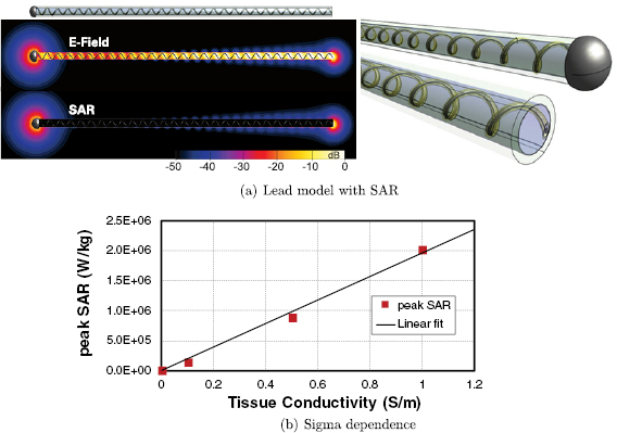
Figure 1. (a) Generic model and specific absorption rate (SAR) distribution of an abandoned neuro-stimulator lead which features a helical wire structure embedded in insulating material around an air-filled core. One end consists of a large electrode, the other is the cut lead with a small cross-section of the wire exposed. (b) Tissue conductivity dependence of the peak spatial-average SAR (psSAR) at a realistic incident field strength of 150 V m−1 (64 MHz).
Download figure:
Standard image High-resolution image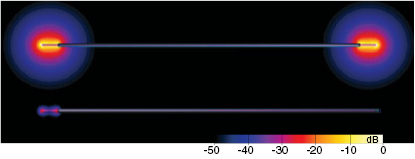
Figure 2. Simulated electric field distribution induced near the lead tips for a partially insulated straight wire with both tips uncapped (top) and with one tip capped (bottom). Note the strong field reduction at the uncapped tip when the other end is insulated.
Download figure:
Standard image High-resolution image1.3. Objectives
The objectives of this paper are to:
- identify a suitable mechanistic description and quantitative model for electrically small implants exposed to electromagnetic (EM) fields
- validate that model by means of in silico methods, including detailed simulations of the exposure inside inhomogeneous human computational anatomical models
- study the impact of various factors, such as lead length, tip shape, tissue dielectric properties, and frequency
- derive lessons learned and formulate suitable approaches for safety assessment standardization, guidelines, and procedures for use across a wide frequency range.
2. Methods
2.1. Theory
Based on the above observations for electrically small implants—i.e. implants that are small compared to the resonance length of  , where λ is the wavelength in tissue—the following mechanistic picture for insulated, elongated implants is proposed: current is driven through the implant, which offers little resistance and acts as short-circuit between exposed implant locations (e.g. contact electrodes or cut wires). The current is either driven by the potential difference (electrical exposure) or the electromotive force (magnetic exposure); in both cases, the tangential E-field integrated along the implant is relevant. Resistance principally results from the finite conductivity of the tissues surrounding the implant tips, where current must squeeze through the tissue into the small, exposed surface of the implant conductor. Thus, the setup can be viewed as a serial arrangement of two resistances (R1,2, where the indices 1 and 2 distinguish the two implant ends) that exhibit inverse dependence on the conductivity of the local tissue (σ) and only weak dependence on tip shape (s):
  , where f(si) is a function that describes the dependence of resistance on tip shape and the index
  again serves to distinguish the two ends. The total current produced is
  . The local current density at a location x near the tip is
  , where the distribution
  can be determined by solving the electro-quasistatic equation (
 , where ϕ is the electric potential).
  depends on the tip shape and is normalized such that the tip-surface integral of it equals 1. Volume averaging of
  is expected to remove most of the dependence on tip shape. The E-field is obtained as
  and the SAR is
  , where ρ is density. Equations (1)–(4) summarize the mechanistic theory.


The behavior of temperature increase resembles that of averaged SAR quantities with regard to how it depends on dielectric tissue properties, implant shape/trajectory, and in vivo field conditions. In the absence of thermoregulation, the temperature increase distribution linearly depends on the power deposition distribution and thermal diffusion introduces spatial smoothing akin to that of spatial SAR averaging. There is, however, an additional dependence of temperature increase on thermal properties (especially perfusion). With regard to neuro-stimulation, the relevant quantities (Reilly et al 2011) are the averaged E-field—for end-node stimulation—and the activating function, which is related to the E-field Jacobian, for center-node stimulation.
The suggested alternative mechanistic picture explains why the field enhancement is dramatically reduced when one end of the lead is surrounded by insulating material.
For homogeneous tangential E-field exposure of magnitude E in homogeneous tissue, the newly introduced mechanism predicts that  ,
,  , and
, and  , which reproduces and explains the observed linear dependence on σ. When the tissue conductivity at the second implant end is twice that of the first end (
 ), the prediction is that similar currents are produced at both ends, but that the E1 and SAR1 at the first end of the wire are twice the magnitude of the E2 and SAR2 at the second end. An increase in J of 4/3 is expected in comparison to a homogeneous setup with
  .
.
For bare implants, the current can enter and leave at any location along the lead, which reduces the current density, field strength, and SAR. This effect is partly compensated by the reduced resistance that increases the total current (see section 4.2).
With increasing frequency, (i) the length of the implant becomes increasingly large relative to the wavelength, making resonance and field-phase effects important when the half-wavelength becomes comparable to the implant length, and (ii) capacitive coupling through the insulation becomes relevant, such that the insulation thickness becomes important and the behavior of thinly insulated implants begins to resemble that of bare implants.
2.1.1. Determination of  and
and


 can easily be computed by solving the quasi-static equation in homogeneous medium under homogeneous exposure conditions and normalizing the current density
  distribution by the total (integrated) current J that leaves the tip. However, the determination of
  can be more complex. If both tip-shapes are identical,
  can simply be determined using equation (1). If the two tip-shapes differ, an additional semi-homogeneous simulation must be performed, in which the conductivity of the region around one of the tips is changed. Application of equation (1) to the two simulations results in a system of two equations for f(s1) and f(s2) that can be solved analytically or numerically. This approach can be generalized to more than two 'tips', in which case as many (semi-)homogeneous simulations as tips are required. In these simulations the combinations of local tissue conductivities around the tips must be linearly independent to obtain a uniquely solvable set of equations.
2.2. Simulations
2.2.1. Homogeneous electric exposure
To test and validate the proposed mechanistic model, a range of simulations were performed on simple, straight insulated wires of radius 0.75 mm with bare tips (ASTM 2182-11 a (2011), figure 3) exposed to a homogeneous field, while varying the:
- overall tissue conductivity: 0.05–0.77 S m−1, relevant for muscle, fat, heart, and grey matter in the frequency range under study (table 1, based on Gabriel et al (1996) and Hasgall et al (2016)); default: muscle
- frequency: 3 kHz–128 MHz
- tip shape: see figure 4; default: 10 mm of straight, bared wire as in the IEC 60601-2-33 (2010) standard; while some of these tip shapes are realistic (helical, sharp), others have been selected because they are either standardized (IEC 60601-2-33 (2010)), or to generically cover a wide variety of tip shapes and potentially relevant features (sharp versus spherical, short versus long)
- implant length: 100–800 mm; longer for the analysis of phase gradient
- insulation thickness: 0–1 mm; default: 0.5 mm
- structure of the lead: straight versus helical
- local tissue conductivity: one or both tips embedded in cylindrical muscle tissue with twice the background conductivity
- phase gradient of the tangential E along the lead: 0–5 rad m−1

Figure 3. Sketch of the straight semi-insulated wire used for analysis of the E-field exposure.
Download figure:
Standard image High-resolution imageTable 1. Tissue conductivity values in (S m−1) at studied frequencies; based on Gabriel et al (1996) and Hasgall et al (2016).
| Tissue | 3 kHz–10 MHz | 10 MHz | 64 MHz | 128 MHz |
|---|---|---|---|---|
| Muscle | 0.33–0.72 | 0.62 | 0.69 | 0.72 |
| Fat | 0.05–0.07 | 0.053 | 0.066 | 0.070 |
| Heart muscle | 0.50–0.77 | 0.50 | 0.68 | 0.77 |
| Grey matter | 0.29–0.59 | 0.29 | 0.51 | 0.59 |
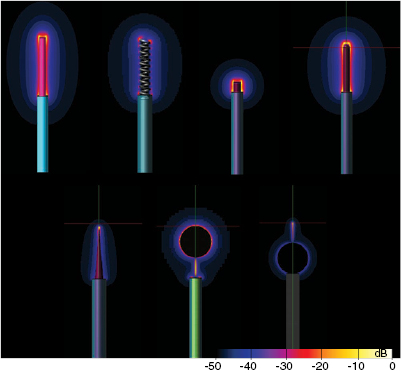
Figure 4. Induced E-field distributions at the lead tips for different tip shapes.
Download figure:
Standard image High-resolution imageFor frequencies >10 MHz, the finite differences time domain (FDTD) method of Sim4Life v.3.0 (ZMT Zurich MedTech AG, Switzerland) was used to perform simulations (Taflove et al 2005). The partially insulated leads were exposed to uniform plane waves with the E-field tangential to the lead. A plane-wave source box was placed at a distance of 30 mm from the lead, and the perfectly matched layer (PML) boundary condition was used to truncate the computational domain after 20 mm. For the phase gradient simulations, the Huygens Box source functionality of Sim4Life was used to define the corresponding incident field conditions. The computational domain was discretized with a rectilinear grid of 1 mm resolution and refinement of 0.5 mm in the tip region. A convergence analysis was performed for the case of a 10 cm wire at 64 MHz by varying the tip region resolution from 0.2–0.9 mm in five steps and computing the variability of the averaged quantities-of-interest (see section 2.2.4), which is found to be <3%. The deviation between the standard resolution and the highest resolution is also <3%.
For frequencies ⩽10 MHz, where the wavelength is much larger than the length of the implant, the finite element method (FEM) simulator of Sim4Life was used to solve the electro-quasistatic (EQS) approximation (suitable when:  and
and  , where ω is the angular frequency,
  the electric permittivity, σ the electric conductivity, μ the magnetic permeability, and d the characteristic length of the computational domain). The suitability of the EQS approximation was verified against FDTD simulations at 10 MHz, the most critical (highest) frequency: for all quantities-of-interest (QoI, see below), the deviation remains <0.13 dB (1.5% for
  ,jav, J and 3% for psSAR), even for the longest lead. Only the unaveraged
  -field, which is very sensitive due to steep gradients (figure 5), was found to deviate by up to 0.9 dB (11%).
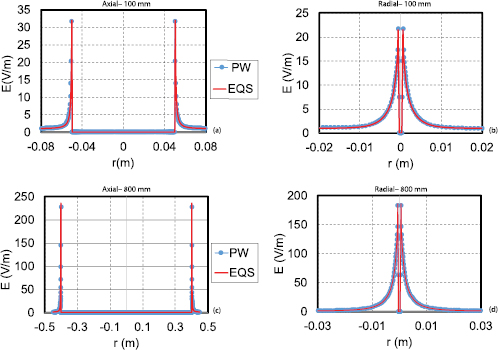
Figure 5. Comparison of E-field obtained by FDTD plane-wave modeling and EQS uniform exposure modeling. The E-field shown is that along the long axis of the wire ((a), (c)), as well as radially through the middle of the tip ((b), (d)) for wires of length 100 mm ((a), (b)) and 800 mm ((c), (d)).
Download figure:
Standard image High-resolution imageIn all cases, the background exposure (field in the absence of the implant) was subtracted before computing the QoI, to assess the impact of the presence of the implant.
2.2.2. Magnetic exposure
To investigate magnetic exposure, two wires of circular cross-section were embedded along trajectories forming circular arcs in a cylindrical muscle tissue and were exposed at frequencies ⩽10 MHz to circularly symmetric fields generated by a current loop. The insulated wires (wire radius: 0.75 mm, insulation thickness: 1 mm) with bare tips (10 mm exposed) were inserted along trajectories with constant, tangential E-fields. One wire covered one-quarter and the other three-quarters of a circle of radius 17.5 cm. The mesh had an overall resolution of 1 mm with refinements of 0.3 mm near the wire and of 0.5 mm in the regions around the tips.
2.2.3. In vivo exposure
To confirm the validity of the model in realistic inhomogeneous setups, simulations involving detailed anatomical models and a realistic implant were performed. The male adult human computational anatomical model 'Fats' from the Virtual Population (ViP) (Gosselin et al 2014) was used in combination with the model of an abandoned neuro-stimulator lead shown in figure 1. It features an insulated helical wire structure embedded in additional insulating material around an air-filled core. One end consists of a large and rounded electrode and the other ('tail') is the cut lead with only a small cross-section of the wire exposed. The implant models were positioned on the left and right of the spine, based on medical images of a patient. The right one was completely embedded in muscle, while the left one was partly in muscle (tail) and partly in fat (electrode). In all cases, the tissue environment was inhomogeneous, involving tissue interfaces with high dielectric contrast (e.g. to bone) in implant proximity. Exposure to E and magnetic (B) fields was simulated (figure 6). The B-field originated from a 10-turn rectangular spirangle coil, while electric exposure was to a capacitively-applied, longitudinally-oriented E-field. Tissue dielectric properties were assigned according to published values for exposure at 100 kHz (Hasgall et al 2016). Simulations were performed with the magneto-quasistatic and the ohmic-current dominated EQS solvers on a mesh with body resolution of 2 mm, refinement of 0.5 mm in the tip regions, and refinement of 0.03 mm of the wire and insulation. To determine  and
and  (see section 2.1), two simulations were performed: homogeneous implant exposure within a homogeneous medium (0.5 S m−1) and semi-homogeneous exposure within two half-spaces (0.5 S m−1 and 0.1 S m−1). For the semi-homogeneous exposure the electrode was embedded in the 0.5 S m−1 medium and the tail in the 0.1 S m−1 medium. From these two simulations, in vivo J and psSAR at the electrodes and tails of the left and right implant were estimated, using the mechanistic model and computed incident field conditions from electric and magnetic exposure in the absence of implants. For additional validation, another semi-homogeneous exposure simulation with inverted implant orientation was performed and compared to the model predictions.
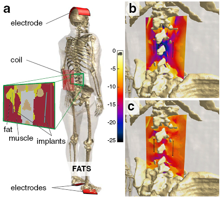
Figure 6. Setup for the validation of the mechanistic model involving exposure of the detailed human ViP anatomical model Fats with integrated implants to a coil-sourced B-field or to a capacitively applied E-field (a). Illustrative E-field distributions are shown for the magnetic (b) and electric (c) exposures.
Download figure:
Standard image High-resolution image2.2.4. Quantities of interest
The following quantities were extracted from the EM exposure simulations: (i) the maximum induced  , SAR, and
  at the lead tip; (ii) the peak of the E-field vector averaged on a cube of 2 mm side according to ICNIRP 2010 (
 , (ICNIRP 2010)); (iii) the peak of the E-field vector averaged over a 5 mm long straight line (
 , (IEEE C95.1 2005)); (iv) the peak of the induced current
  averaged over a disc of 1 cm2 surface (
 , (ICNIRP 1998)); (v) the psSAR in cubes of 0.1, 0.5, 1, and 10 g tissue mass (psSAR
 , psSAR
 , psSAR
 and psSAR
 ); and (vi) the total current J.
  ,
,  ,
,  , and psSAR are standardized quantities that are routinely used in safety assessment.
2.2.5. Temperature increase
In addition, thermal simulations were performed, using the EM simulation results as sources, to assess the temperature increase after one hour of exposure. The temperature increase was estimated by solving the thermal diffusion equation with the transient thermal solver in Sim4Life:

where T is the temperature, t the time, k the thermal conductivity, and C the specific heat capacity. Table 2 summarizes the thermal tissue property values employed. As in Kyriakou et al (2012), thermal conduction along the implant and heat removal by perfusion were not considered to obtain conservative results. See Kyriakou et al (2012) for an analysis of their impact.
Table 2. Thermal tissue properties (density (ρ), heat capacity (C), thermal conductivity (k)) according to Hasgall et al (2016).
| Tissue | ρ (kg m−3) | C (J/kg/K) | k (W/m/K) |
|---|---|---|---|
| Muscle | 1040 | 3550 | 0.53 |
| Fat | 911 | 2348 | 0.21 |
| Heart muscle | 1081 | 3686 | 0.56 |
| Grey matter | 1045 | 3696 | 0.55 |
3. Results
3.1. Electric exposure
3.1.1. Normalized electric quantities
The QoI described above were extracted in all simulations of homogeneously exposed insulated straight wires with bare tips for frequencies <10 MHz and normalized according to the expected dependencies (equations (1)–(4)) on the tissue- and frequency-dependent σ, lead length, and incident field strength, in line with the proposed mechanism. The variability of the normalized psSAR, E,  ,
,  , and
, and  is small; the coefficients of variation (standard deviations normalized by means) of the dependence on frequency, σ, and length are <2%, <5%, and <5%, respectively, over an 8-fold range of length. The small variability supports the proposed mechanistic model of voltage-driven current through an implant short circuit. Accordingly, differences of ⩽5% are found between the simulated quantities and those obtained by rescaling a single simulation (800 mm lead at 10 MHz) according to the expected dependence on material properties and implant length (see figure 7).

Figure 7. Comparison of simulated and predicted frequency (affects tissue conductivity), and implant length dependence of psSAR (a); the reference simulation used for the predictions is the 800 mm lead at 10 MHz. The relative difference is shown in (b).
Download figure:
Standard image High-resolution image3.1.2. Normalized temperature increase
The ratio of temperature to SAR is stable for all muscle cases (coef. of var. <1%), but—as expected—it is affected by the different thermal and perfusion properties of other tissues. For example, at 10 MHz, the temperature to SAR ratio of fat is higher than that of muscle by 26%.
3.1.3. Tip environments
When σ is doubled locally at one wire tip, the local SAR is expected to change by a factor of (4/3)2/2 (equation (4)). The 1g and 10g averaged SAR show deviations from the expected change by 1% and 5%, respectively. Insulation of one end of the lead reduces the SAR by a factor >100 at a frequency of 1 MHz. When the frequency is increased from the low frequency regime to MRI frequencies, this insulation efficacy is reduced as capacitive coupling across the insulation becomes possible (as discussed in section 4.2), e.g. at 128 MHz deposited power near the tip is reduced by a factor of four.
3.1.4. Electrical length
With increasing electrical length, the normalized temperature increase and averaged SAR quantities (e.g. psSAR , according to equation (4)) are no longer independent of length and frequency, as resonance and phase phenomena become relevant. Figure 8 shows the length and frequency dependence of psSAR0.1g in a plot that is directly comparable to figure 6 from Kyriakou et al (2012). While the focus of Kyriakou et al (2012) is on higher frequencies and that of this paper on lower ones, there is visual agreement in the results of the two data sets in the overlapping frequency range. When the normalized quantities are plotted as a function of the electrical length lE (lead length normalized by the 'wavelength'
  of thin, insulated antennas embedded in lossy media, according to equation 13(b) of King et al (1974)), the values change substantially for
  –0.3 (see figure 9(a)). A universal scaling behavior is apparent for insulated implants embedded in muscle tissue. Comparison of the rescaled behavior curves in muscle and in fat tissues reveal very similar values for non-thermal quantities below
  –0.3, but differ strongly for longer electrical lengths. A resonance is apparent in fat tissue at
  , but absent in muscle tissue—this is likely due to dampening of the resonant mode by electrical losses in the conductive medium along the implant (
 ), when the fields surrounding the insulated implant become non-negligible at resonance. Figure 9(b) shows similarly rescaled curves for bare implants; the psSAR values at the tips of the bare wire decay rapidly at electrical implant lengths much shorter than the lengths at which the psSAR values of partially insulated wires drop. While universal behavior is still apparent in muscle tissue, it is not as consistent as that seen with insulated implants. In conclusion, the proposed mechanistic model is valid for insulated implants with electrical lengths
  . Values for the electrical length
  at varying frequencies can be found for different tissues in table 3, which also puts
  in relationship to the tissue-specific wavelength
  (where
  and
and  denotes the imaginary part).
  considers the impact of the metal wire and its dielectric insulation on the 'wavelength', while λ only accounts for the dielectric tissue properties.

Figure 8. Length and frequency dependence of psSAR0.1g for comparison with figure 6 from Kyriakou et al (2012); there is visual agreement between the two sets of results in the overlapping frequency range.
Download figure:
Standard image High-resolution image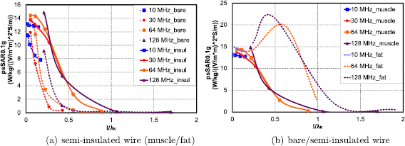
Figure 9. psSAR as a function of the electrical length for lead exposures at frequencies ranging from 10–128 MHz, normalized according to the expected dependency on lead length, frequency-dependent tissue conductivity, and tangential E-field. Impact of (a) tissue environment (fat versus muscle) and (b) insulation (bare versus partially insulated wire).
Download figure:
Standard image High-resolution imageTable 3.  (computed for insulation thickness of 0.5 mm) in different tissues over frequencies ranging from 0.15–128 MHz;
  is the effective wavelength of thin, insulated antennas embedded in lossy media, according to King et al (1974). The wavelength (λ) is also provided for comparison.
| Freq. (MHz) | Muscle | Fat | Grey matter | |||
|---|---|---|---|---|---|---|
 (m) (m) |
λ (m) |  (m) (m) |
λ (m) |  (m) (m) |
λ (m) | |
| 0.15 | 290 | 12 | 280 | 39 | 280 | 20 |
| 1 | 47 | 4.0 | 44 | 15 | 46 | 6.8 |
| 10 | 5.2 | 2.1 | 3.7 | 4.8 | 5.1 | 1.4 |
| 64 | 0.9 | 0.4 | 0.8 | 1.1 | 0.9 | 0.4 |
| 128 | 0.5 | 0.3 | 0.4 | 0.6 | 0.5 | 0.2 |
3.1.5. Temperature increase to SAR ratio
The ratio of temperature increase to SAR is not affected by length or frequency, showing a variation <5% for partially insulated wires and <7% between partially insulated and bare wires for all analyzed lead lengths and frequencies.
3.1.6. Insulation
At 10 MHz, the insulation thickness (varying between 0.1–1 mm) has a minimal impact on psSAR and induced E-field (<5%). However, as discussed before, the normalized quantities decrease with increasing frequency, and that decrease is steeper for bare wires. With decreasing insulation thickness, thinly insulated wires start to behave more like bare wires the higher the frequency (see figure 10), because, at higher frequencies, capacitive coupling through the insulation becomes increasingly important and thin insulation layers less relevant.

Figure 10. Normalized psSAR0.1g as a function of frequency for insulation thicknesses of 0, 0.1, 0.5 and 1 mm.
Download figure:
Standard image High-resolution image3.1.7. Tip shape
The impact of the tip shape of electrically short implants on the normalized quantities was investigated at 10 MHz, and more important variability than that observed for the other parameters was observed: 14% (coefficient of variation) for psSAR1g, 22% for psSAR10g, 7% for temperature increase, 11% for EICNIRP. The variability in peak E is high (60%), with a clear trend towards higher fields for sharper tip shapes. The variability of temperature increase in muscle of only 3% is likely due to the smoothing effect of thermal diffusion. The variability in the averaged quantities for electrically short implants is sufficiently small as to void the necessity for tip-specific analysis. However, the variability increases substantially in implants that are not electrically short. The tip-shape-dependent correlation between peak E, EICNIRP, or averaged SAR and temperature has been determined for a 20 cm lead at 10 MHz. The highest correlation is found for averaged SAR quantities (slightly higher for 0.5 g than for other averaging masses). The main configuration that reduces correlation is the short (2 mm) tip, but this case is an outlier: the two field maxima, one at the end of the insulation and the other at the end of the tip, are distinct on the field level or for very small averaging volumes, but contribute jointly to 1 g- and 10 g-averaged SAR values (due to the averaging volume) and temperature (due to thermal diffusion).
3.1.8. Helical wire
At 10 MHz, replacing the straight lead with a helical wire has only a minor impact (2–13%) on the averaged SAR quantities, EICNIRP and temperature increase. However, a helical wire behaves very differently with higher frequencies: at 64 MHz, the decrease in 0.1 g averaged SAR for the 20 cm helical wire is a factor of four greater than that for the straight wire, and at 128 MHz, the difference is a factor of 20. This reflects the increased effective length of the helical wire—in comparison with the straight wire—which now becomes comparable to the resonance length.
3.1.9. Phase gradient
With increasing length, the phase gradient also starts to be relevant. Figure 11 shows (for partially insulated lead wires of varying length) the normalized variation in induced E-field at the lead tip under application of an incident 10 MHz field of constant strength with a constant phase gradient along the implant, as a function of the phase gradient. For lead lengths on the order of  (2.6 m; shorter at higher frequencies or for coiled leads), phase-gradient effects are increasingly important. The worst-case phase gradient is actually non-zero, which is equivalent to a complex-valued transfer function.
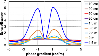
Figure 11. Induced E-field at the lead tip for different implant lengths as a function of incident field phase gradient (normalized by the zero gradient, homogeneous exposure value); computed at 10 MHz in muscle;  m.
m.
Download figure:
Standard image High-resolution image3.2. Magnetic exposure
As expected, the three-quarter circle wire in the circularly symmetric setup results in j and E-field values that are three times higher (nine times higher for SAR) than those with the quarter circle wire, in agreement with expectations for current driven by an electromotive force.
3.3. Exposure in an anatomical environment
To validate the model proposed in section 2.1 in complex, inhomogeneous body environments (as relevant for safety assessments), simulated implant-related energy depositions and field enhancements at the two ends (electrode and cut lead tail) of abandoned neuro-stimulator leads near the spine of an anatomical model under electric and magnetic exposure (see section 2.2.3) were compared to predictions from the proposed model. Those predictions were derived by combining (i) characterization of the electrode and tail behavior in two simple and (semi-)homogeneous environment and exposure conditions (to determine  and
and  ; see sections 2.1 and 2.2), (ii) information about the tissue conductivities at the electrode and tail locations (right implant: muscle conductivity at both ends; left implant: fat conductivity at the electrode and muscle conductivity at the tail), and (iii) the integrated tangential incident in vivo fields, according to equation (4). (i) revealed that
  is 30 times larger than
  , due to the reduced resistance to current entering the large electrode compared to the resistance of entering the small exposed wire cross-section of the cut lead. The psSAR
 , psSAR
 , and psSAR
 at the two implant ends, for electric and magnetic exposure, and for the two anatomical implant placements show an averaged signed deviation from the numerically obtained reference values of 0.1% (i.e. there is no systematic bias), a coefficient of variation of 7%, and a maximal deviation of 15%, thus supporting the proposed mechanistic model and demonstrating its predictive value.
3.4. Summary of results
The results show that, for electrically short and sufficiently insulated implants, normalization according to the mechanistic model results in averaged electrical QoIs that have no significant dependence on tissue properties, implant length, exposure strength, and field inhomogeneity along the lead, although there is a weak dependence on tip shape. The normalized temperature increase shows additional dependence on thermal properties around critical implant locations. Thus, relevant QoI for electric and magnetic exposure safety can be predicted, even for the in vivo case, from a single reference simulation in (semi-)homogeneous tissue per tip-shape. Only when the electric length of the implant becomes comparable to the resonance length—at about 0.2–0.3 —do the structure of the lead, the phase gradient, and interactions with the tissues surrounding the insulated part of the lead become important.
4. Discussion
The results presented demonstrate that, while the transfer function approach commonly applied for MRI safety assessments of elongated implants is not suitable for electrically short implants, the mechanistic model based on currents driven through an implant short-circuit and limited by the resistive tissue surrounding exposed implant locations can successfully predict energy deposition and field enhancement (at least for the averaged quantities commonly employed in safety standards). The new model is valuable not only for MRI safety assessment of small implants and abandoned leads, it is rather a general model for electrically short implants that covers low-frequency exposure safety assessments for implant-wearers, e.g. in the context of WPT technologies.
4.1. Standardization
This new mechanistic model and the findings in support of it suggest an approach that may possibly be used to assess electrically short implants for device testing procedures, safety guidelines, and standardization according to the following steps:
- (i)A single reference simulation, or experimental measurement, per tip-shape of homogeneous exposure within a (semi-)homogeneous tissue is performed to characterize the tip-related resistance and field distribution ( and ).
- (ii)In vivo incident field conditions are determined (these could be precomputed for the relevant exposure scenarios and reused for different devices).
- (iii)The local exposure metrics are predicted, based on the mechanistic model, by combining the reference simulation with the in vivo incident field conditions and information about the tissues surrounding critical exposed implant locations.


Another benefit of this model and approach is, that it becomes possible to identify potential worst-case conditions:
- Case 1:When (i) exposed implant locations (tips or electrodes) are all in a given tissue or medium (e.g. blood), (ii) differences in the electrical conductivity at the possible anatomical positions are small, or (iii) a single, conservative conductivity value is assumed:
- Case 1a: For electric exposures at low frequencies, electro-quasistatic solvers can be employed to determine the E-field potential. The worst-case condition for a lead-like implant is obtained by identifying the pair of points that correspond to relevant, possible lead end-points that have the largest potential difference.
- Case 1b: At higher frequencies or for magnetic exposures, the electro-quasistatic approximation is not suitable and an electric potential cannot be defined. The worst-case is obtained by identifying the relevant lead trajectory with the maximal integrated tangential E-field.
- Case 2:When the electrical conductivity of potential anatomical locations for exposed implant conductors cannot be considered as constant/given: the above procedure (finding worst-case potential difference or integrated tangential E-field) is extended by considering the conductivities at the exposed locations according to equations (1)–(4).
4.2. Insulation
The mechanistic model has been derived for elongated implants that are insulated except for two exposed locations. The presence of the insulation reduces the area of the implant surface through which current can enter and exit to those exposed locations. While this increases the overall resistance and hence reduces the total current J, it also causes the current flux to be concentrated in a smaller area or volume. The results presented show that the total effect is one of higher local energy deposition for insulated implants than for bare implants. Thus, effective insulation is a worst-case condition.
4.3. Tip tissue environment
The implant can be embedded in homogeneous tissue or have a trajectory that crosses different tissues (e.g. a pacemaker that is routed through a blood vessel and has a helical tip which is screwed into heart muscle). The proposed mechanism does not need to know about the dielectric properties along the insulated lead (only the tangential E-field or the voltage difference), yet it requires knowledge about the tissue environments at the exposed tips. Should that environment itself be inhomogeneous (i.e. involve tissue interface in close proximity to the tip), the determination of the resistance  is affected and the normalized current density distribution
  will be distorted. Further investigations are needed to determine if the resulting effective R and averaged
  can be assumed to be averages of the ones in the different tissues, such that for example only the worst-case tissue could be considered, or if additional considerations are required.
5. Conclusions
The exposure of people with medical implants to EM fields is highly relevant since current guidelines for general EM exposure safety do not take this population group into account. The problem was first addressed for the MRI product standard (ISO-TS 10974:2012 (2012)). However, the transfer function approach employed for elongated implants has been found to be unsuitable for electrically short implants ( ). In this study, we have developed a quantitative, generalized EM safety model for electrically short conductive implants that is suitable for a wide range of frequencies (applied in this paper to WPT and MRI exposure scenarios, covering the range 3 kHz– >100 MHz). For insulated or partially insulated leads up to ∼0.2 times the effective wavelength, the amount of power deposited at the implant tips depends on the voltage difference or electromotive force between the two tips and is a simple function of the local tissue resistivity at the tips, and only weakly dependent on tip shape. The phase gradient and interactions with tissue surrounding the insulated part of the lead only needs to be considered when the electric implant length becomes comparable to the resonance length of the lead.
Simulations of homogeneous exposure in simple environments, as well as of setups involving realistic implants embedded in complex anatomical environments under exposure to E- or B-fields were used to validate the model. For the investigated in vivo electric and magnetic exposure cases, the proposed model is capable of predicting psSAR with an accuracy in the order of 7% (maximal deviation <15%) based on only two simulations of homogeneous implant exposure within (semi-)homogeneous environments.
The mechanistic model provides valuable support for the formulation of a general approach for use in safety guidelines and standards that is applicable for exposure to EM fields over a large frequency range. It also suggests a possible approach for the identification of worst-case implant routing conditions.
Further research will be performed to develop tools to conservatively (with minimal overestimation) determine compliance with basic restrictions for real wave exposure scenarios.
Acknowledgments
The results presented have been developed partly in the framework of the 16ENG08 MICEV Project. The latter received funding from the EMPIR Programme co-financed by the Participating States and from the European Union's Horizon 2020 Research and Innovation Programme.