
Abstract
The aim of this work was to determine magnetic field correction factors that are needed for dosimetry in hybrid devices for MR-guided radiotherapy for Farmer-type ionization chambers for different magnetic field strengths and field orientations. The response of six custom-built Farmer-type chambers irradiated at a 6 MV linac was measured in a water tank positioned in a magnet with magnetic field strengths between 0.0 T and 1.1 T. Chamber axis, beam and magnetic field were perpendicular to each other and both magnetic field directions were investigated. EGSnrc Monte Carlo simulations were compared to the measurements and simulations with different field orientations were performed. For all geometries, magnetic field correction factors, , and perturbation factors were calculated. A maximum increase of 8.8% in chamber response was measured for the magnetic field perpendicular to chamber and beam axis. The measured chamber response could be reproduced by adjusting the dead volume layer near the chamber stem in the Monte Carlo simulations. For the magnetic field parallel to the chamber axis or parallel to the beam, the simulated response increased by 1.1% at maximum for field strengths up to 1.1 T.

A complex dependence of the response was found on chamber radius, magnetic field strength and orientation of beam, chamber axis and magnetic field direction. Especially for magnetic fields perpendicular to beam and chamber axis, the exact sensitive volume has to be considered in the simulations. To minimize magnetic field correction factors and the influence of dead volumes on the response of Farmer chambers, a measurement set-up with the magnetic field parallel to the chamber axis or parallel to the beam is recommended for dosimetry.

Original content from this work may be used under the terms of the Creative Commons Attribution 3.0 licence. Any further distribution of this work must maintain attribution to the author(s) and the title of the work, journal citation and DOI.
1. Introduction
Hybrid magnetic resonance (MR) guided radiotherapy devices provide radiation treatments in combination with excellent soft tissue contrast imaging without adding any additional dose of ionizing radiation to the patient. Therefore, they have the potential of further improving radiation therapy outcome by offering the possibility to adapt the treatment according to the actual patient anatomy and potential motion. Currently, several devices are in clinical use or in development, which use combinations of 60Co sources or 6 MV linacs with a 0.35 T, 0.5 T, 1.0 T or 1.5 T MRI (Lagendijk et al 2008, Fallone 2014, Keall et al 2014, Mutic and Dempsey 2014). MR-linacs with 3 T are very conceivable and diagnostic MR devices with this field strength are frequently used. For these devices, diagnostic images will be superior to low-field MRIs and the electron return effect was shown to be smaller (Raaijmakers et al 2008). However, distortions in images of high-field MRIs need to be investigated separately.
In order to integrate these devices into clinics, accurate dose calculations and dosimetric measurements in strong magnetic fields for treatment planning and quality assurance are needed. The magnetic field of the MRI can, however, influence the response of dosimeters.
Reference dosimetry is mainly performed with air-filled ionization chambers. Due to the Lorentz force acting on the electrons, electron trajectories inside the sensitive volume of the chamber are altered and this changes the chamber response. Therefore, a new formalism for reference dosimetry in magnetic fields with appropriate correction factors has to be established.
Meijsing et al performed experiments and Monte Carlo simulations of dosimetry with the NE2571 Farmer chamber in magnetic fields and found an increase of up to 8% and 11% at 1 T, depending on the orientation of the chamber with respect to the radiation beam (Meijsing et al 2009). They showed that the change in response could be correlated with the modified number of electrons entering the cavity and their average path length in the cavity. In another study, Smit et al analyzed the response of the same ionization chamber in a 1.5 T MR-linac prototype and reported an increase in chamber reading of 4.9% (Smit et al 2013). As demonstrated by Reynolds et al, the change in response depends on the magnetic field strength, the ionization chamber and the orientations of magnetic field, chamber axis and radiation beam (Reynolds et al 2013).
To correct for the effects of the magnetic field, a new correction factor in accordance with the IAEA TRS-398 dosimetry protocol (Andreo et al 2006) can be applied. This correction factor can be calculated by means of Monte Carlo simulations for a user beam quality Q, and accounts for the change of the chamber response in the presence of a magnetic field B (O'Brien et al 2016).

In this work, the response of six Farmer-type ionization chambers of different radii was measured in an experimental electromagnet for various magnetic field strengths. These data were compared to EGSnrc Monte Carlo simulations and were used to adjust the dead volume layer near the chamber stem in the simulations. After this adjustment, the response of the chambers was simulated and the magnetic field correction factors, , as well as the perturbation factors were calculated for different magnetic field strengths and field orientations.

2. Materials and methods
2.1. Ionization chambers
For the study, six Farmer-type chambers, including the PTW 30013 (radius 3 mm) and five custom-built ionization chambers with the same design, but varying inner radii from 1 mm to 6 mm, were used (see figure 1(d)). The behavior of these chambers has been described previously by Legrand et al (2012a, 2012b). The cavity length of all chambers is 23 mm. The wall consists of a 0.335 mm thick PMMA layer which is coated with graphite of 0.09 mm thickness. The central electrode has a diameter of 1.15 mm and a length of 21.2 mm and is made of aluminum. The chamber stem is built of layers of various materials, including PMMA, graphite and aluminum, among others. In the following, the chambers are referred to as Ri (where i = (1, 6), corresponds to their inner radius).

Figure 1. (a) Picture of the experimental set-up with the beam of the linac being incident from the rear direction. (b) Sketch of the experimental set-up. (c) The water tank with integrated circulation system. The water flows through the tank from the bottom to the top (red arrows) and is then removed via pipes integrated into the tank walls (green arrows) (Bakenecker 2014). (d) Picture of the six Farmer-type chambers of varying radii. (e) µCT scan of the R3 chamber.
Download figure:
Standard image High-resolution image2.2. Experimental set-up
The charge reading per monitor unit (MU) of the six Farmer-type chambers was measured in magnetic fields. Therefore, the chambers were positioned in a self-designed and 3D-printed water tank (material: VeroClear RDG810, density: 1.18–1.19 g cm−3, size ca. 3.5 × 12 × 15 cm3, see figures 1(a) and (b)) with their reference point at 10 cm water equivalent depth in accordance with the TRS-398 dosimetry protocol (Andreo et al 2006). Thus, a layer of 5 cm water was used for backscatter material. The bias voltage of the chambers was set to 400 V. The thickness of the water tank was limited to 3.5 cm, such as to fit between the pole shoes of the electromagnet (Schwarzbeck AGEM 5520, Germany). The maximally achievable magnetic field strength was 1.1 T. A description of the magnet can be found in Stefanowicz et al (2013). A water circulating system was integrated into the water tank to limit the increase of the water temperature due to heating of the magnet to less than 0.2 °C per measurement series.
The chambers were positioned with 3D-printed holders that fixed the chamber stem at the top of the water tank. Care was taken to ensure that there were no air bubbles near the sensitive volume of the chambers.
All irradiations were performed with 100 MU using a horizontal beam of the 6 MV linear accelerator (linac, Artíste, Siemens Medical Solutions Inc., PA, USA). A maximum field strength of below 1 mT was measured at the linac head. Thus, no influence of the magnetic field on the beam generation was assumed. The source to surface distance (SSD) was set to 100 cm. To avoid significant back scatter from the pole shoes of the electromagnet, a radiation field of 3 × 10 cm2 was used.
The magnetic field was oriented perpendicular to the beam as well as to the chamber axis. The magnetic field strength ranged between 0.0 T and 1.1 T, corresponding to electric currents from 0.0 A to 14.11 A, respectively. Each set of measurements of different field strength was repeated three times with a randomized order of magnetic field strength to avoid systematic effects from magnetic hysteresis.
2.3. Monte Carlo simulations
2.3.1. Simulation geometry.
The Farmer-type chambers were modeled using the C++ class library egspp of the Monte Carlo code EGSnrc (Kawrakow 2000, Kawrakow et al 2009). The materials and dimensions of the chambers were obtained from data sheets provided by PTW (details see section 2.1) and µCT images (Inveon®, Siemens, Germany). The stems of the chambers were modeled in detail according to the µCT scans (see figure 1(e)). In particular, care was taken to ensure that any air gaps in the chamber stem were modeled correctly. The ionization chamber models were placed in a 50 × 50 × 50 cm3 water phantom. The reference points of the chambers were positioned at reference depth, i.e. at 10 cm water-equivalent depth, in accordance with the TRS-398 protocol (Andreo et al 2006). As beam source, a 6 MV photon spectrum collimated to a field size of 3 × 10 cm2 was used (Mohan et al 1985). According to the experimental set-up, an SSD of 100 cm was used. A schematic drawing of the simulation set-up is displayed in figure 2.

Figure 2. Schematic drawing of the simulation geometry: Radiation beam is directed in +Z-direction, chamber axis in Y-direction and magnetic field in X-direction. FL indicates the average direction of the Lorentz force. (a) Magnetic field in −X-direction. (b) Magnetic field in +X-direction.

Download figure:
Standard image High-resolution imageThe calculation of the dose to the sensitive chamber volume was performed using the egs_chamber user code (Wulff et al 2008b). To reduce calculation time, variance reduction techniques such as local photon cross-section enhancement and range-based Russian Roulette were employed.
Homogeneous magnetic field strengths ranging from 0.0 T to 3.0 T were used in the simulations, employing a customized magnetic field macro (provided by Dr Kawrakow, see appendix for Fano cavity test results with this magnetic field macro). To assure correct simulation of the electrons in the magnetic field, a maximum step length of 0.025 times the gyration radius of the electron was used.
Moreover, a maximum global energy loss in an electron step of ESTEPE = 0.1 and a maximum first elastic scattering moment per step of XIMAX = 0.1 were used. Spin-off effects were turned off. The default transport cut-off energies were used (ECUT = 0.521 MeV, PCUT = 0.01 MeV).
2.3.2. Definition of dead volumes.
In a first step, the whole air volume below the guard electrode was considered to belong to the sensitive volume, i.e. the dose was scored in this volume. For all chambers R1 to R6, the response was calculated and compared with the measurements in magnetic fields ranging from 0.0 T to 1.1 T. The magnetic field was oriented in X-direction, perpendicular to the beam and the chamber axis (see figure 2).

To investigate the dose distribution within the sensitive volume in detail, the air volume of the R3 chamber was divided into small ring-shaped volumes (radii 0.1, 0.15, 0.2, 0.25, 0.305 cm and heights of either 0.01 cm or 0.05 cm). In an additional simulation, the ring scoring zone around the reference point of the chamber was divided into six equal azimuthal sections. Simulations were performed for magnetic field strengths of 0.0 T, −1.0 T and +1.0 T.
Especially close to the stem of the ionization chamber, the electric field is likely to be not perfectly uniform, such that a reduced charge collection efficiency is expected. A small part of the air volume adjacent to the guard electrode may act as a 'dead volume', i.e. the charge created within this part is not scored. This was simulated by excluding cylindrical slabs of the air volume and adapting the height of this volume in 0.01 cm steps for each chamber until a good agreement with the measurement was obtained.
2.3.3. Magnetic field orientation.
Using the adapted dead volumes of the chamber models, the chamber response was also studied for other magnetic field orientations that could not be realized with our experimental set-up. The response of the six chambers in magnetic fields in Y- and Z-direction (Y: perpendicular to the beam and parallel to the chamber axis/Z: parallel to the beam) was calculated for magnetic field strengths ranging from 0.0 T to 3.0 T.
2.3.4. Calculation of and perturbation factors.

To correct for the altered chamber response in magnetic fields, as well as perturbation factors were calculated. The correction factor for the beam quality Q obtained for the reference field can be calculated as the ratio of dose to water Dw and measured signal M with and without magnetic field B (O'Brien et al 2016). Assuming that the mean energy deposited in air per Coulomb charge does not change with magnetic field strength, factors can be calculated with Monte Carlo simulations by


where Dchamber denotes the dose to the air volume of the chamber.
Moreover, the dose to water Dw can also be expressed as

where pQ denotes the overall perturbation factor, sw,air the averaged stopping power ratio of water and air and pstem, pcel, pwall, and prepl represent the perturbation factors due to the stem, central electrode, wall and replacement, respectively. The perturbation factors were calculated as described by Wulff et al (2008a). The approach is illustrated in figure 3.

Figure 3. Calculation scheme for the determination of the perturbation factors, adapted from Wulff et al (2008a).
Download figure:
Standard image High-resolution imageTo calculate the correction factor and perturbation factors under reference conditions, the 10 cm × 10 cm IAEA phase space of a 6 MV Siemens Primus linac (Pena et al 2007) was used as beam source. The remaining simulation geometry and parameters were set as described in section 2.3.1.

The dose to water Dw at the point of measurement was calculated in a water-filled cylindrical volume of 1 cm radius and 0.025 cm height.
The averaged stopping-power ratios between water and air were determined with the help of the user code SPRRZnrc (Rogers et al 2013) in a water phantom at the depth of measurement. An electron cut-off energy of 10 keV was used (Wulff et al 2008a).
3. Results
3.1. Response of Farmer-type ionization chambers in magnetic fields
The measured relative signal of the charge reading per MU in the presence of the magnetic field to the response without magnetic field is depicted in figure 4 for all six chambers and both magnetic field orientations perpendicular to beam and chamber axis. The chamber response shows a complex dependence on magnetic field strength, chamber radius and magnetic field orientation. For the chambers R3 to R6, the response increases up to a certain magnetic field strength and decreases beyond. The maximum increase in +X-direction was observed for chamber R4 at 0.9 T (8.8%), while in the ‒X-direction the maximum increase was obtained for chamber R3 at 1.0 T (7.0%). Moreover, switching the magnetic field orientation has only a minor influence on the response of the small chambers (R1–R3, around 1%), whereas the impact increases for chambers with larger radii (up to 6% for the R6 chamber). The magnetic field strength at which the maximum response occurs decreases for increasing chamber radii.

Figure 4. Dependence of the measured chamber response on the magnetic field strength for the magnetic field in X-direction. Panel (a) shows the results for chambers R1–R3, panel (b) for R4–R6. The error bars state the measurement uncertainty (standard deviation of three measurements plus the uncertainty for temperature and pressure as well as the reading uncertainty). Horizontal error bars show the uncertainty in magnetic field strengths, measured for a given coil current with a hall probe and randomized order in coil currents. Some error bars are smaller than the symbols.

Download figure:
Standard image High-resolution imageFigure 5 shows the results of the simulations for chambers R3 and R6, when the sensitive volume is considered to consist of the whole air volume below the guard electrode in the chamber. The measured response is shown for comparison. In contrast to the measurement, the increase in chamber response is slightly larger in the ‒X-direction than in the +X-direction. Moreover, the difference in response between both magnetic field orientations is smaller in the simulations. Particularly for the R6 chamber, a large disagreement between measurement and simulation can be observed.

Figure 5. Measured and simulated response in the presence of the magnetic field in X-direction for the chambers (a) R3 and (b) R6, when the sensitive volume is considered to consist of the whole air volume below the guard electrode in the chamber.

Download figure:
Standard image High-resolution image3.2. Influence of dead volumes
In order to investigate the influence of dead volumes, the spatial dose distributions in the air volume of the chambers were analyzed. The results for chamber R3 are presented in figure 6.

Figure 6. Spatial dose distribution within the air volume of the chamber R3 for 0.0 T (panels (a) and (d)), −1.0 T (panels (b) and (e)) and +1.0 T (panels (c) and (f)) in X-direction. Panels (a)–(c) show the dose scored in azimuthal rings around the chamber axis (Adapted from Spindeldreier et al (2017), Copyright 2017, with permission from Elsevier.), while panels (d)–(f) show the dose scored in discretized azimuthal segments around the reference point (located at Y = 0 in panel (a)–(c)). Doses are normalized to the mean dose at 0.0 T.
Download figure:
Standard image High-resolution imageThe statistical uncertainty (standard deviation) of all scoring regions is below 0.4%, with a mean uncertainty of 0.2%. Figures 6(a)–(c) show the resulting dose maps integrated over the azimuthal sections for 0.0 T, −1.0 T and +1.0 T in X-direction, respectively. If no magnetic field is applied, the dose distribution inside the air volume is rather homogenous (figure 6(a)). In contrast, when a magnetic field of 1.0 T is applied in the ‒X-direction, dose hot spots of up to +35% and cold spots of −20% relative to the mean chamber dose without magnetic field are found at the guard electrode and at the chamber tip, respectively. This effect is simply due to deflection of the electrons towards the chamber stem by the Lorentz force. The opposite effect occurs for a 1.0 T magnetic field in the +X direction. Here, low dose regions are formed at the chamber stem, while high dose regions are found at the chamber tip.
Figures 6(d)–(f) display the dose distribution for 0.0 T, −1.0 T and +1.0 T in the transversal plane at the reference point for discretized azimuthal segments. The beam is directed from bottom to top of the figures. The statistical uncertainty of all scoring regions is below 0.7%, with a mean uncertainty below 0.4%. Without magnetic field, the dose distribution is again rather homogeneous, showing only a small dose decrease at the beam exit behind the central electrode. In the presence of a magnetic field, the dose is concentrated at the beam entrance side with dose hot spots of about +35%, while dose cold spots of −26% are observed at the beam exit side originating from the lateral deflection of secondary electrons.
Thus, the assumption of a cylindrical dead volume at the guard electrode can lead to a significant change in the simulated chamber response.
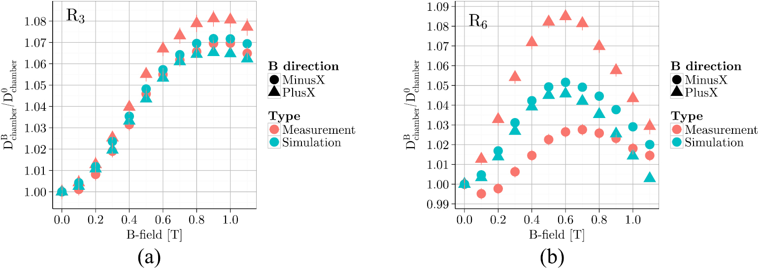
Figure 7 displays the simulation results of the response for the R3 chamber with cylindrical dead volumes of different thicknesses adjacent to the guard electrode. The larger the dead volume, the larger is the difference in response between the +X and –X magnetic field orientation: The response for the +X-direction increases with an increase in thickness of the dead volume, since the low dose region (see figure 6(c)) is excluded, while the effect is opposite for the ‒X-direction due to the exclusion of the high dose region close to the chamber stem (see figure 6(b)). Therefore, it was possible to adapt the simulation results to the measurements by adjusting the thickness of the dead volume. Figure 8 shows the best fit of the thickness of the dead volumes for all six chambers. The thickness of the dead volumes for the R1, R2, R3, R4, R5 and R6 are 0.08 cm, 0.09 cm, 0.11 cm, 0.19 cm, 0.22 cm and 0.26 cm, respectively. A very good agreement between measurement and simulation was obtained with a root-mean squared deviation of 0.2% and a maximum deviation of 0.9% for the R4 chamber at 1.1 T in +X-direction.

Figure 7. Simulated response of the R3 chamber for various dead volume thicknesses as a function of the magnetic field strength in X-direction.

Download figure:
Standard image High-resolution image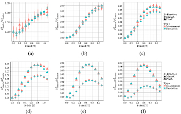
Figure 8. Measured and simulated response of all chambers for a magnetic field oriented in X-direction. The simulated data was computed considering a cylindrical dead volume adjacent to the guard electrode in the simulation. (a) R1. (b) R2. (c) R3. (d) R4. (e) R5. (f) R6.

Download figure:
Standard image High-resolution image3.3. Influence of the magnetic field orientation
With the simulation models adapted to the measurement, the response was investigated also with respect to the magnetic field orientations that could not be realized by means of our experimental set-up. Figures 9 and 10 display the dose distribution inside the air cavity of the chamber R3 for a 1.0 T magnetic field in Y (parallel to the chamber axis) and Z direction (parallel to the beam). Only minor changes relative to the dose distribution without magnetic field can be observed along the chamber axis. The doses increase slightly in vicinity of the central electrode and towards the guard electrode. In the transversal plane, the dose distribution is disturbed according to the Lorentz force: For a magnetic field in Y-direction and electrons traveling in beam direction, the Lorentz force points on average in X-direction, thus hot (up to +34%) and cold spots (down to −39%) arise at the X sides of the chamber (see figures 9(d)–(f)). For a magnetic field in Z-direction, one can observe a dose increase at the beam entrance side of the chamber (see figures 10(e) and (f)) (up to +9%).


Figure 9. Calculated dose distribution within the chamber R3 for a magnetic field in Y-direction. Panels (a)–(c) show the dose scored in azimuthal rings around the chamber axis, while panels (d)–(f) show the dose scored in discretized azimuthal segments around the reference point (located at Y = 0 in panel (a)–(c)). Doses are normalized to the mean dose at 0.0 T.

Download figure:
Standard image High-resolution image
Figure 10. Calculated dose distribution within the chamber R3 for a magnetic field in Z-direction. Panels (a)–(c) show the dose scored in azimuthal rings around the chamber axis, while panels (d)–(f) show the dose scored in discretized azimuthal segments around the reference point (located at Y = 0 in panel (a)–(c)). Doses are normalized to the mean dose at 0.0 T.

Download figure:
Standard image High-resolution imageThe corresponding responses for the magnetic field in Y- and Z-direction are shown in figure 11.


Figure 11. Simulated chamber response of all chambers with adapted sensitive volume for magnetic fields in Y- (a) and Z-direction (b).


Download figure:
Standard image High-resolution imageFor a magnetic field in Y-direction, the chamber response again describes a complex dependence on magnetic field strength, chamber radius and field orientation. The dependence on the field orientation, however, is much smaller than for the case where the chamber axis is perpendicular to the beam and the magnetic field. The response of the small chambers R1 and R2 increases by +1.3% for 3.0 T. For the larger chambers, a maximum response evolves, whose magnitude and position depend on the chamber radius. The larger the chamber radius, the smaller is the perturbation of the chamber response. It can be noted that for an increasing chamber radius, the magnetic field strength at which the maximum perturbation occurs decreases. The largest chamber, R6, exhibits a maximum increase of the response of +0.3% at 0.7 T. Since the ionization chamber models are rotationally symmetric and the electron energy fluence points mostly in beam direction, no significant dependence on the magnetic field orientation in Y-direction is found.

For a magnetic field in Z-direction, the response increases monotonically with an increasing magnetic field. The chamber response changes only slightly, around +1.0% for 1.0 T. Except for chamber R1, no significant dependence on the chamber radius and the magnetic field orientation can be observed for this geometry.

3.4. Calculation of and perturbation factors

The magnetic field correction factors calculated for a 10 × 10 cm2 reference field for all three magnetic field directions using equation (1) are shown in figure 12. Numerical values of the commercial R3 chamber (PTW 30013) are given in table A1 (supplementary material (stacks.iop.org/PMB/62/6708/mmedia)). Since the dose to water changes only slightly with increasing magnetic field strength (around −0.3% for a 1.0 T field in X-direction/−0.2% for 1.0 T in Y-direction/+0.1% for 1.0 T in Z-direction), the graphs reveal approximately the inverse shape of the response curves. For a magnetic field perpendicular to beam and chamber axis (X-direction), decreases towards a minimum, depending on the chamber radius (maximum change of −7.6% for the R4 chamber at 0.8 T), and rises again for higher magnetic field strengths.


Figure 12. correction factors for all chambers and different magnetic field orientations. (a) B-field in X-direction. (b) B-field in Y-direction. (c) B-field in Z-direction.


Download figure:
Standard image High-resolution imageWith a magnetic field parallel to the chamber axis (Y-direction), also first decreases towards a minimum with increasing magnetic field strength. In this case, smaller chamber radii exhibit a larger decrease (maximum decrease −2.5% for the smallest R1 chamber at 3.0 T). The correction factor of the largest chamber R6 reduces only by about −0.5% at 0.7 T, before rising again towards unity. For a magnetic field parallel to the beam (Z-direction), decreases monotonically with increasing field strength, presenting a decrease of about −0.8% at 1.0 T. Only minor influence of the chamber radius can be observed for this configuration.


The perturbation factors associated with the chamber stem, central electrode, wall and replacement of the water by air are shown in figure 13 for all six chambers and for a magnetic field in X-, Y- and Z-direction, respectively. All perturbation factors show a clear dependence on the chamber radius, magnetic field strength and orientation. However, only for a magnetic field oriented along the X-direction an influence of the magnetic field orientation on the perturbation factors was found.


Figure 13. Stem perturbation factor pstem (.1), perturbation factor of the central electrode pcel (.2), wall perturbation factor pwall (.3) and replacement perturbation factor prepl (.4) for all chambers and different magnetic field orientations (in X-direction (a), in Y-direction (b) and in Z-direction (c)). Most of the error bars (statistical uncertainty) are smaller than the symbols.


Download figure:
Standard image High-resolution imageThe magnetic field in +X-direction causes a steeper increase in the stem perturbation factor pstem than a field in ‒X-direction, since in this case, the electrons in the water region replacing the chamber stem are deflected towards the cavity where they deposit additional dose. The stems of the R1 and R2 chambers were built slightly differently from the other chamber stems, which may be the reason for the small shift in their pstem perturbation factors compared with the other ones. For a magnetic field in Y-direction, pstem decreases monotonically for the R1 and R2 chambers (maximally by −0.7% at 3.0 T for the R2 chamber), while it monotonically increases for the chambers R4–R6 (maximally by +0.9% at 3.0 T for the R6 chamber). A magnetic field in Z-direction causes pstem to approach towards unity for all chambers at a high magnetic field strength.


The central electrode perturbation factor pcel presents again a maximum depending on the chamber radius for a magnetic field in X-direction. The field orientation has only a minor impact on pcel, however. The highest variation in pcel due to the field direction is observed for the R1 chamber with +3.6% at 1.5 T. For the case of the magnetic field in the Y-direction, a minimum perturbation factor is observed for the large chambers. In contrast, for a magnetic field in Z-direction, pcel decreases monotonically for higher field strengths. For both cases of the field in Y- and Z-direction, however, the smaller the chamber radius, the higher is the deviation from unity of pcel. The largest decrease can be found for the R1 chamber with −1.5% at 3.0 T for a magnetic field in Y-direction.


The wall perturbation factor pwall increases for all magnetic field directions with increasing field strength by about 1–2% at 3.0 T, except for the +X-direction. For this direction, pwall first decreases slightly by about −0.2% to 0.7–0.8 T for the R3–R6 chamber, before increasing again for higher field strengths. The increase in pwall is shallower for the +X-direction, when the electrons enter the cavity from the chamber stem side, compared to the −X-direction, as there is no wall in this region and thus less perturbation. The pwall value is smaller for smaller chamber radii.
The replacement perturbation factor prepl shows a minimum, depending on the chamber radius, for a magnetic field in X-direction, before it increases again at higher field strengths. The maximum decrease can be observed for the R5 chamber with −8.0% at 0.6 T. This perturbation factor is the main contributing factor to the correction factor showing a very similar shape to . For a magnetic field in Y- and Z-direction prepl, changes only slightly, decreasing monotonically with increasing field strength.


4. Discussion
4.1. Response of Farmer-type chambers in magnetic fields
A complex behavior of the chamber response curves was found in measurements and simulations depending on the chamber radius and the magnetic field strengths as well as on the field direction. As described by Meijsing et al, this behavior can be explained by the number of electrons, their track length and their energy dependent stopping power inside the chamber air cavity (Meijsing et al 2009). The average number of electrons entering the chamber cavity depends on the magnetic field direction, since more electrons can reach the sensitive volume via the stem and the dead air volume than via the chamber tip. The larger the chamber radius, the larger is the difference in the number of electrons entering the cavity for the two magnetic field directions. In general, the average number of electrons reaching the sensitive volume decreases with the magnetic field in −X-direction and exhibits a maximum for magnetic fields in +X-direction, as can be seen in figure 14(a).

Figure 14. Dependence of the (a) mean number of electrons and (b) mean track length inside the sensitive air volume of the Farmer-type chambers (excluding the dead volume) on the magnetic field strength for the magnetic field in X-direction.

Download figure:
Standard image High-resolution imageThe average electron track length within the cavity rises with increasing magnetic field strength up to a certain field strength, before decreasing again for higher magnetic field strengths (see figure 14(b)). The larger the chamber, the smaller is the maximum increase in track length relative to that at 0 T. A possible explanation may be the decreasing surface to volume ratio with increasing radius. As expected, no significant influence of the magnetic field direction on the mean track length was observed.
4.2. Influence of the dead volume
The size of the sensitive volume has an important impact on the response curve of Farmer-type chambers in magnetic fields, especially when the average direction of the Lorentz force is along the chamber axis. As the electric field inside the chamber air cavity may be disturbed, especially close to the guard electrode, dead volumes can occur, reducing the size of the sensitive volume. A reduction of the electric field near the chamber stem and thus the existence of dead volumes was also observed by Butler et al (2015). They studied dose maps of several chambers, including a PTW 30013 Farmer chamber that corresponds to the R3 chamber used in the present study, and found that there is a signal reduction near the chamber stem, which can be explained by a decreased electric field. The charge created in these dead volumes is then not collected by the central electrode, but e.g. by the guard electrode. Therefore, these volumes have to be excluded from the sensitive chamber volume in the simulations. In our simulations, the dead volumes were approximated as cylindrical volumes. Realistic dead volumes, however, might be more toroidal-shaped due to the electric field distribution at the guard electrode.
The adjusted dead volume has to be considered as an effective dead volume and its determination is also affected by inherent limitations of efficient Monte Carlo particle transport, i.e. the cut-off energies.
In principle, the adjustment of the dead volume in the Monte Carlo simulation could also be affected by the orientation between the magnetic field and the ionization chamber, as the simulation does not consider trajectories of electrons with energies below 10 keV. In a measurement, however, different magnetic field orientations may change the angular distribution of these low-energy electrons and thus the measured charge.
If the average direction of the Lorentz force lies in the plane perpendicular to the chamber axis, however, the residual range of low-energy electrons is expected to be of minor importance as in this case, the electrons are not deflected towards or away from the guard electrode and therefore the dose distribution is more homogeneous in the cavity including the dead volume near the guard electrode.
In contrast, if the Lorentz force is on average directed along the chamber axis, hot or cold dose spots arise within the dead air volume. Therefore, excluding the air volume near the guard electrode from the sensitive volume in the simulation changes the chamber response curve significantly. In this work, the thickness of the simulated dead volume was adjusted until measured and simulated chamber response curves agreed. Experimentally, the dead volume can in principle be determined by scanning the chamber across a small slit beam or with a step-like dose profile and measuring the signal (Butler et al 2015, Ketelhut and Kapsch 2015). With this method, dosimetric response maps can be determined. However, the measurement has to be very precise to be able to detect dead volume below 1 mm in height for the R1 chamber. Moreover, to investigate the effect of the magnetic field, a set-up of this experiment in a magnetic field would be desired. Therefore, the scope of this work was to develop virtual chamber models that reproduce the response measurements rather than the exact measurement of the sensitive volumes of the chambers. These models were further-on used to study other orientations of chamber, beam and magnetic fields.
4.3. Influence of the magnetic field orientation
The response curve for a magnetic field parallel to the chamber axis or parallel to the beam revealed smaller changes compared with the case of a magnetic field perpendicular to beam and chamber axis. Again, the changes in response can be explained by the average track length and the number of electrons inside the sensitive volume: For a magnetic field in Y-direction, the average electron path length inside the cavity increases slightly with increasing field strength, whereas the amount of electrons decreases for higher field strengths. Both values increase continuously for a magnetic field in Z-direction. Moreover, no dependence on the field orientation could be observed for a field in Y- or Z-direction. A magnetic field in Y-direction causes a Lorentz force on average in X-direction, thus along the rotationally-symmetric direction of the chamber. Therefore, no change in response can be observed when reversing the orientation of the field in the simulation. In reality, the chambers might be not perfectly rotationally-symmetric, which might have an influence on the response when reversing the magnetic field in Y-direction. A magnetic field in Z-direction leads to a focusing of electrons along the +Z-direction for both orientations and thus to no changes in response for both Z-directions.


Therefore, a set-up with a magnetic field parallel to the chamber axis or, if possible, parallel to the beam would be better suited for reference dosimetry in magnetic fields since smaller correction factors would be needed and simulations would be less error-prone when potential dead volumes are not simulated correctly. This agrees with the findings of O'Brien et al, stating that the correction factors are minimized, when the chamber is aligned parallel to the magnetic field (O'Brien et al 2016).
However, when recommending a set-up for reference dosimetry, the influence of a misalignment of the chamber needs to be considered. Smit et al performed measurements with a Farmer ionization chamber in a magnetic field rotating from a parallel alignment of chamber and magnetic field towards a perpendicular alignment: They showed that for a chamber set-up parallel to the magnetic field a misalignment of 10 degrees changes the response by less than 0.6%, whereas such a misalignment causes a change in response of only 0.4% for a chamber set-up perpendicular to the field (Smit et al 2013). This suggests a similar impact of set-up uncertainties for both alignments, but a detailed analysis of the influence of realistic set-up uncertainties on dose measurements in magnetic fields still needs to be performed.
4.4. Calculation of and perturbation factors

Magnetic field correction and perturbation factors can be calculated with the help of Monte Carlo simulations. It was found that the correction factors can be minimized by selecting the magnetic field in Y- or Z-direction, i.e. oriented along the chamber axis or along the beam direction. As elaborated upon already in sections 4.1 and 4.3, this effect can be explained by the number and the path length of the electrons entering the cavity.


For the same reason, the changes of the perturbation factors are largest for magnetic fields in X-direction. For this direction, pstem and pwall vary around 1%, pcel around 4%. The largest influence factor on the overall perturbation factor and thus on the magnetic field correction factor , is prepl, with changes of up to −8.0%. For a magnetic field in Y-direction, pstem changes by about 1%, and pcel, pwall and prepl by about 2%. The smallest changes in perturbation factors can be found for a magnetic field in Z-direction with variation in pstem of around 0.2%, and of around 1% in pcel, pwall and prepl.


In general, for most of the investigated directions the absolute values of the chamber stem, central electrode and chamber wall perturbation factors deviate the most from unity for smaller chamber radii. The chamber wall as well as the central electrode are largest relative to the chamber radius for the small chamber R1, thus they have the biggest influence for this chamber.
In the current IAEA protocol, the stem perturbation factor is ignored in the kQ calculation (Andreo et al 2006). This is acceptable without a magnetic field since the pstem value differs only by below 0.4% from unity. However, applying a magnetic field of 1.5 T in +X- or of 3.0 T in Y-direction can change this factor to values that differ by around 1% from unity depending on the magnetic field direction and the chamber radius. Thus, for these field orientations, the pstem factor should be included in the calculation. For a magnetic field in Z-direction, the pstem factor is close to unity, thus in this case the stem perturbation factor may still be ignored.


The central electrode perturbation factor changes with magnetic field strength and decreases with field strength for a magnetic field in Y- and Z-direction, since here, more electrons can reach the electrode and thus more perturbation occurs at higher field strengths. In contrast, the pwall perturbation factor increases at higher magnetic field strengths. Again, more perturbation occurs, since more electrons reach the cavity, when no wall is present. The pwall factors for the R1 and R2 chamber are below unity without magnetic field, because parts of their walls were slightly modified by the vendor to fit the chamber stem that was adapted from the R3 chamber.
4.5. Experimental and simulation set-up
Our experimental set-up deviates in some points from the recommended set-up for reference dosimetry. The radiation field size was limited to a 3 × 10 cm2 compared to the reference 10 × 10 cm2 field size. To estimate the effect of the different field sizes, a simulation with both field sizes was performed. The calculated magnetic field correction factors for a 3 × 10 cm2 and a 10 × 10 cm2 field differed maximum by only 0.4% for all investigated magnetic field strengths.
For the calculation of the magnetic field correction and perturbation factors, given in the results, the 10 × 10 cm2 reference field was used.
The experimental electromagnet itself had an influence on the measurement due to scattering. With the magnet (without magnetic field) around the phantom, +1.1% more signal was recorded than without the magnet (Bakenecker 2014). However, since relative measurements have been performed, this should have no significant effect on the measured values.
Hackett et al and Agnew et al described that small air gaps have a large effect on measurements with ionization chambers (Hackett et al 2016, Agnew et al 2017). In addition to the visual check for air bubbles, the response of the R3 chamber was measured three times within a time period of several months. A very good reproducibility of the response measurements with a maximum deviation of 0.3% ensured that no accidentally trapped air perturbed the measurement.
The PTW 30013 chamber (R3) was also used by Agnew et al for measurements in magnetic fields irradiated with a 60Co source (Agnew et al 2017). For comparison of our simulation chamber model, the response measurement was simulated using a 10 × 10 cm2 field produced with a 60Co spectrum (Rogers et al 1988). Although the simulation was performed in water instead of the experimental Perspex phantom and a different SSD was used, a good agreement with a mean squared difference of 0.4% was obtained (maximum difference 0.7%), confirming our chamber model.
In the chamber response simulation described in section 2.3.1, a 6 MV spectrum was used as beam source. To estimate the influence of small differences in the spectrum, correction factor calculations were performed for the R3 chamber with different 6 MV spectra from the literature (spectrum of an Elekta SL25 (Sheikh-Bagheri and Rogers 2002) as well as spectra produced from the IAEA phase space files of Siemens Primus (Pena et al 2007), Varian Clinac 600C (Brualla et al 2009), Varian Clinac iX linacs): The factor calculated for 10 × 10 cm2 field sizes generated with the different spectra differed on average by 0.1% (maximum difference 0.5%). Thus, small changes in the beam spectrum have only a small influence on the factors.


5. Conclusions
In this work, magnetic field correction factors for Farmer-type chambers are calculated for different magnetic field strengths and field orientations. The response of the chambers has a complex dependence on chamber radius, magnetic field strength and the orientation between radiation beam, chamber axis and magnetic field. The largest changes in response and thus in correction factors were observed for a magnetic field perpendicular to beam and chamber axis.
Additionally, for this magnetic field orientation, the exact definition of the sensitive volume of the chamber is important, since the Lorentz force deflects electrons towards or away from dead volumes close to the guard electrode. It was found that a set-up with the magnetic field parallel to the chamber axis or parallel to the beam provides is more robust, since the correction factors as well as the influence of dead volumes are minimized.
Acknowledgments
This project has received funding from the EMPIR programme co-financed by the Participating States and from the European Union's Horizon 2020 research and innovation programme. Detailed information on the chamber geometry provided by Dr E Schuele and R Kranzer (PTW) are gratefully acknowledged. Moreover, we thank the DKFZ core facility small animal imaging for providing the µCT data. We would also like to express our gratitude towards our colleagues Armin Runz and Gernot Echner who developed and 3D-printed the water container and the detector mountings and Dr P Häring, M Splinter and C Lang who facilitated the linac measurements.
Appendix. Fano cavity test with the magnetic field macro
To test the Monte Carlo simulations with magnetic field macro for consistency, the Fano test in a magnetic field can be applied (Bouchard and Bielajew 2015, Bouchard et al 2015, de Pooter et al 2015). For this test, a primary source of 1.25 MeV electrons, isotropically distributed and uniform per unit mass, was used. The geometry consisted of the R3 chamber, positioned in the center of a cylinder of either water, PMMA or graphite with the same density. Therefore, the chamber stem and wall were set to the surrounding medium. The cavity and the central electrode consist of the same medium as the enclosing cylinder but with a 1000 times smaller density. Simulations without magnetic field and with a magnetic field of 1.0 T and 3.0 T strength in −X, −Y and −Z-direction were performed. The dose was scored in the cavity and compared to the expected result of , with I the number of electrons per unit mass and E0 the initial electron energy (Malkov and Rogers 2016).

The deviation from the expected results for water, PMMA and graphite are presented in figure A1. For all magnetic fields, the simulated result agrees to within 0.13% with the expected result. It can be concluded that the magnetic field macro does not perturb the consistency of the simulations.

Figure A1. Relative deviation of cavity dose from the expected result for different media and magnetic field geometries. (a) Water. (b) PMMA. (c) Graphite.
Download figure:
Standard image High-resolution image