

Abstract
Fibroglandular tissue volume and percent density can be estimated in unprocessed mammograms using a physics-based method, which relies on an internal reference value representing the projection of fat only. However, pixels representing fat only may not be present in dense breasts, causing an underestimation of density measurements. In this work, we investigate alternative approaches for obtaining a tissue reference value to improve density estimations, particularly in dense breasts.
Two of three investigated reference values (F1, F2) are percentiles of the pixel value distribution in the breast interior (the contact area of breast and compression paddle). F1 is determined in a small breast interior, which minimizes the risk that peripheral pixels are included in the measurement at the cost of increasing the chance that no proper reference can be found. F2 is obtained using a larger breast interior. The new approach which is developed for very dense breasts does not require the presence of a fatty tissue region. As reference region we select the densest region in the mammogram and assume that this represents a projection of entirely dense tissue embedded between the subcutaneous fatty tissue layers. By measuring the thickness of the fat layers a reference (F3) can be computed. To obtain accurate breast density estimates irrespective of breast composition we investigated a combination of the results of the three reference values. We collected 202 pairs of MRI's and digital mammograms from 119 women. We compared the percent dense volume estimates based on both modalities and calculated Pearson's correlation coefficients.
With the references F1–F3 we found respectively a correlation of  ,
,  and
and  . Best results were obtained with the combination of the density estimations (
 ).
).
Results show that better volumetric density estimates can be obtained with the hybrid method, in particular for dense breasts, when algorithms are combined to obtain a fatty tissue reference value depending on breast composition.
Export citation and abstract BibTeX RIS
1. Introduction
Mammographic breast density has been identified as an important risk factor for developing breast cancer (McCormack and dos Santos Silva 2006, Vachon et al 2007, Eng et al 2014). Eng et al showed that the breast cancer risk is highly correlated to automated breast density measurements. Breast density was assessed in four density categories, and the breast cancer risk was up to 8.26 times higher for women with dense breasts (category 4) compared to women with non-dense breasts (category 1). Furthermore, it has been shown that sensitivity of mammography decreases with an increase of breast density (Boyd et al 2007, Kerlikowske 2007, Kerlikowske et al 2015, Prummel et al 2016, Wanders et al 2016). Low sensitivity of mammography in women with dense breasts is explained by the fact that a tumor can be masked by the presence of fibroglandular tissue (also referred to as dense tissue), which is a combination of connective tissue structures and epithelial tissue. Fibroglandular and cancerous tissues have a similar attenuation for x-rays, and thus appear equally white in the mammogram while fatty tissue appears almost transparent.
Breast cancer screening programs are established in many countries. Starting at an age of 40–50 years, these programs offer women periodical breast cancer screening exams with mammography. Personalized breast cancer screening depending on familial risk and breast density, involving other modalities such as ultrasound or MRI, is under discussion (Schousboe et al 2011, Saadatmand et al 2012, Ho et al 2014). Screening with MRI is already recommended for women with a lifetime risk of more than 20–25% (Saslow et al 2007, Mann et al 2008). To implement personalized screening based on density, accurate and objective methods to estimate breast density need to be available.
Different methods have been developed to estimate the amount of fibroglandular tissue in the breast. An overview of automatic mammographic density segmentation techniques has been published recently (He et al 2015). The methods can be categorized in two types: area-based and volume-based methods. Area-based methods (Byng et al 1994, Li et al 2007, Torrent et al 2008, Oliver et al 2010) were developed to objectively reproduce the density categories described in the Breast Imaging Reporting and Data System (BI-RADS) (D'Orsi et al 2003). The BI-RADS density grade is a four-point scale used by radiologists to estimate the percentage area of fibroglandular tissue that is projected in the mammogram. A major limitation of area-based methods is that the 3D structure of the breast is not taken into account as only the projection of fibroglandular tissue is represented. Therefore, the resulting percentage dense area is not invariant to compression and projection angle. Some area based methods also have the disadvantage that human interaction is required (Byng et al 1994).
To overcome these problems, several methods have been proposed to fully automatically estimate volumetric percent density, defined as fibroglandular tissue volume divided by breast volume, on digital mammograms (DM) (Highnam and Brady 1999, Kaufhold et al 2002, van Engeland et al 2006, Malkov et al 2009, Highnam et al 2010, Alonzo-Proulx et al 2012). These methods employ a physics based model of the x-ray image acquisition process and assume that the breast is composed of two types of tissue: fat and fibroglandular tissue. Eng et al have shown that these breast density estimations correlate well with each other and with breast cancer risk. One of the algorithms used by Eng et al is Volpara (Volpara Health Technologies, Wellington, New Zealand) which is based on the work of Highnam and van Engeland. The methods described in Highnam and Brady (1999) and Highnam et al (2010) and van Engeland et al make use of an internal calibration with a pixel that ideally belongs to the projection of fat only. Only pixels in the breast interior are taken into account when estimating the internal reference value, where the interior is defined as the region where the breast is in contact with the compression paddle, excluding the peripheral region of the mammogram in which the breast thickness is smaller. An important limitation of this calibration approach is that the pixel value used as reference may not be representative for only fatty tissue in the breast interior if the breast is very dense. This leads to an underestimation of the fibroglandular tissue volume and percent density in dense breasts (Kallenberg et al 2012, Wang et al 2013, Gubern-Mérida et al 2014).
The aim of our study is to improve breast density estimation in very dense breasts and to find an approach that gives reliable breast density estimations in all types of breasts. We compared the use of alternative methods for obtaining a fatty tissue reference value. For that purpose, we estimated the fibroglandular tissue volume and percent density with three different reference values on mammography and we compared these estimates to reference breast density estimations obtained from MRI data. We first used a reference value obtained with a small breast interior to avoid that pixels of the periphery are accidentally included. The second method used an enlarged breast interior, which is more likely to include a pixel value that represents the projection of only fatty tissue, but has a larger risk to overestimate the reference value due to inclusion of pixels of the peripheral zone. The third approach is based on the idea that also pixel values representing the largest proportion of fibroglandular tissue may serve as a reference. By estimating the amount of fibroglandular tissue that corresponds to the densest part in the mammogram e.g. the difference between the breast thickness and the amount of subcutaneous fat, the fatty tissue reference value is computed. The aim of the latter method is to deal with very dense breasts. Obviously, this method will fail when the breast is not very dense. To overcome this drawback, we investigated if a combination of the three breast density measurements can lead to an overall improvement of breast density estimation results.
2. Methods
2.1. Preprocessing
All mammograms underwent some steps of preprocessing. First the images were segmented into breast tissue, pectoral muscle (in case of a mediolateral oblique—MLO view) and background (Karssemeijer 1998). Additionally, we performed a thickness correction of the peripheral region. We also determined the Euclidean distance d(r) from each pixel location to the skin-line in the mammographic projection. The distance d(r) is used several times throughout the paper and is needed to define the breast interior.
2.2. Fibroglandular tissue volume
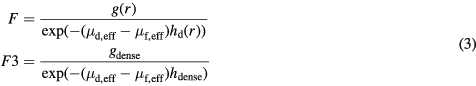
As described in van Engeland et al, the volume of fibroglandular tissue can be computed from unprocessed (raw) digital mammograms based on a physical model of image acquisition and on the assumption that the breast is composed of two types of tissue: dense tissue and fatty tissue. The dense tissue thickness hd at each pixel location can be calculated with the following formula:

where, g(r) is the pixel value at position r and F is the pixel value in a fatty tissue reference region where hd is supposed to be zero. The effective attenuation coefficients,  and
and  for fatty and dense tissue respectively, vary with the breast thickness and with the anode / filter combination of the x-ray tube and are described in van Engeland et al.
The total dense tissue volume (VDT) is given by the integral over the projected breast area B:

2.3. Fatty tissue reference value
In this work, we studied three approaches to obtain an estimate for the pixel value that corresponds to the projection of fatty tissue only. Two reference values (F1 and F2) are based on the pixel value distribution in the breast interior, and the third reference value (F3) was calculated by estimating the proportion of dense tissue in the densest location in the breast. Each approach is explained in the following section.
2.3.1. Reference value F1—the maximum pixel value in a small breast interior region.
To obtain the reference value F1, we used the same approach as described in van Engeland et al The pixel value representative for fatty tissue is determined by taking a large quantile (0.99) of the pixel value histogram computed in the breast interior. We used this approach instead of taking the maximum pixel value, because large pixel values may appear in the mammogram due to artifacts or noise. With this approach the breast interior is rather small and depends on the maximum Euclidean distance computed from the breast pixels to the skin-line. To determine this distance, we first calculate the Euclidean distance from all breast pixels (the pixels that are enclosed by the pectoral muscle boundary, the skin-line and the image edge) to the skin-line. Of these distances we take the maximum. In most cases, the point with the maximum distance to the skin is located on the pectoral muscle or breast boundary, but it is noted that depending on the shape of the breast this point may also be located more inward from the boundary. The interior is then defined as the breast pixels that have at least a distance of 0.4 times the maximum Euclidean distance to the skin-line. An example is shown in figure 1(b).
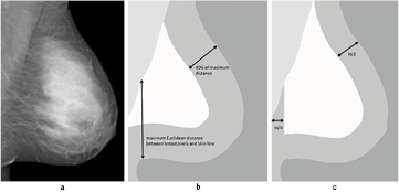
Figure 1. A processed mammogram (a) and the segmentation of breast tissue, pectoral muscle and background (b) and (c). A graphical representation of the small (b) and large (c) breast interior are also shown. The breast interior as defined in (b) is used to compute F1. The breast interior shown in (c) is used for the computation of F2 and F3.
Download figure:
Standard image High-resolution image2.3.2. Reference value F2—the maximum pixel value in a large breast interior region.
In denser breasts, the interior of the breast as defined previously might not contain a pixel representing only fatty tissue. Therefore, we used a second definition of the breast interior region in which pixels closer to the skin-line and located within the fully compressed area are also included.
We defined the larger breast interior as the pixels that have a minimum distance to the skin-line of half the compressed breast thickness (H). Additionally, we excluded pixels that are too close to the vertical image edge, as this region is sometimes not representative due to poor compression, in particular in MLO views. Furthermore, we want to prevent that the pectoral muscle is part of the breast interior in case it is visible in a craniocaudal (CC) view. The breast interior pixels have a minimum distance of a quarter of the breast thickness to the vertical image edge. The breast interior region is given for one mammogram in figure 1(c). To compute the reference value, we again used a large quantile (0.99) of the pixel value histogram. We call this reference value F2.
2.3.3. Reference value F3—an estimate from the densest region (minimum pixel value of the mammogram).
When the breast is very dense, the methods above become inaccurate, as it becomes unlikely that the obtained reference value is representative for the projection of only fatty tissue. In this section, we propose a method to obtain a suitable reference value using the densest region in the mammogram. Given the pixel value corresponding to a dense pixel (gdense) at a certain location r, it is possible to compute the fatty tissue reference value by estimation of the corresponding thickness of dense tissue  . This can be seen if we rewrite formula (1):
The reference value computed in this way is denoted by F3. Note that there is no reference region in the mammogram with this pixel value, but that it can be derived when we can estimate hdense at the location of gdense. To find the reference pixel value gdense, we make use of the large breast interior as used for F2 (see figure 1(c)) and determine the minimum using the 0.01 quantile of the pixel value distribution.
To obtain hdense we have to estimate the amount of fibroglandular tissue that corresponds to the pixel value gdense. Since the reference value gdense corresponds to the densest region in the mammogram, we assume that it represents the projection of dense tissue and the layers of subcutaneous fat. Therefore, this pixel value is also representative for the maximum dense tissue fraction (MDTF) in the compressed breast projection, i.e. the maximum thickness of dense tissue in the path of the x-ray beam divided by the thickness of the compressed breast. Based on this idea hdense is estimated as  with H the compressed breast thickness. To estimate hdense, the MDTF in the direction of the x-ray beam is needed. As this information is unavailable, we calculate the MDTF in the image plane and assume that this value is representative for the MDTF in the direction of the x-ray beam. To make this approach work, two key assumptions need to be fulfilled: (1) in a first approximation the MDTF is direction independent with respect to a rotation around the anterior-posterior axis and (2) that the MDTF does not change when the breast is compressed. In section 3.5 we investigate to what extent these assumptions are valid by using MRI data. The MDTF in the image plane is calculated by constructing paths that represent plausible x-ray trajectories through the breast when it would be decompressed, rotated by 90 degrees, and compressed again. We used slightly curved instead of linear paths, to take into account that when imaging a compressed breast the x-ray beam will be approximately perpendicular to the skin and the subcutaneous fat layer.
The curved paths are defined by taking points on a circle centered at a point (P) outside of the breast. A schematic overview is shown in figure 2. To define this point P, we calculate the minimum distance between the nipple (N) and the pectoral muscle (M). In CC views, we used the vertical image edge instead of the pectoral boundary. The point P has a distance to the nipple of two times the distance NM and lies on the straight line with the points N and M. The nipple is assumed to be located on the skin-line at the position with the maximum distance to the pectoral muscle or the vertical image edge for MLO views and CC views, respectively.
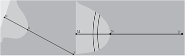
Figure 2. A schematic view of the land marks nipple (N), closest point (M) of the nipple to the pectoral muscle / image edge, for MLO and CC views respectively, and the new point P. In the example of the CC view (right side) are also two curved paths given. All points of a counting path have the same distance to the point P.
Download figure:
Standard image High-resolution imageTo estimate MDTF in the plane of the mammogram we first classify all pixels as dense or non-dense with a Random Forest classifier on a rescaled 200 μm image, using features similar to the ones used in Kallenberg et al (2011). Then, for each path, we count the number of dense and non-dense pixels. To minimize variation we group paths to bands with a width of 0.2 mm with a sliding window approach and calculate the dense tissue fraction of these bands. The MDTF of a mammogram is the absolute maximum of the dense tissue fractions. To estimate hdense, we use the MDTF averaged over all mammograms of an examination (left and right breast, and MLO and CC view), to minimize variation. The MDTF of the MLO and the CC view are assumed to be similar due to the rotation invariance of the MDTF, while the MDTF of the left and right breast are assumed to be similar as the amount of breast density and the breast density distribution of the left and right breast are comparable to each other. Only paths with a minimum distance of NP + H/8 are included, to exclude paths that are too close to the nipple. Furthermore, we exclude paths that are too close to the pectoral muscle to prevent that inaccuracies in the pectoral muscle segmentation influence the result. We also use a distance of H/8 here. Using the thickness of the compressed breast H we estimate hdense by computing  .
.
2.4. Combination of fibroglandular tissue volume estimations
Previous studies showed that the breast density estimates obtained with F1 provide accurate results for non-dense breasts. However, the reference values F2 and F3 were obtained under the assumption that the breast is dense. Hence, it is likely that the breast density estimations obtained with these reference values do not give accurate results in non-dense breasts. In this study, we developed two hybrid approaches that combine the breast density estimations to obtain suitable results for the complete range of breast densities.
The first combination scheme takes only into account results from F1 and F2. Based on the MDTF a threshold t is set. If MDTF is below that threshold, the fibroglandular tissue volume estimate obtained with F1 is used. Otherwise we use results from reference value F2.
The second combination scheme of the breast density estimates involves three parameters (t, a and b) and results from the three reference values are combined. The first parameter is a threshold (t). If MDTF is below that threshold, the fibroglandular tissue volume estimate obtained with F1 is used. In case of a MDTF above that threshold, a linear combination of the other two fibroglandular tissue volume estimations is used, where the weights depend on the MDTF. The combination scheme can be written as

with  and VDT1, VDT2 and VDT3 the dense tissue volumes obtained with the reference values F1, F2 and F3 respectively.
In the evaluation, five fold cross validation was used to obtain optimal values for the parameters. The data set was divided into five groups, or folds, of equal size. To avoid bias all exams of a woman were in the same fold. Then, four folds were used to optimize the parameters, which were then applied on the fifth fold. This process was repeated such that the obtained parameters were once applied to each fold. The parameters were obtained by minimizing the sum of the squared residuals in the comparison of percent density between mammography and MRI averaged per breast.
2.5. Breast volume
In this work, we used two approaches to estimate the breast volume. The first one is based on the semi-circle model (Snoeren and Karssemeijer 2004). In that approach, which was applied in van Engeland et al, the interior is assumed to consist of parallel planes, while the peripheral zone is approximated by semi-circles. The thickness as a function of the compressed breast thickness (H) is given by:

where d(r) is the Euclidean distance between the breast pixel location and the skin-line.
The second breast volume estimate algorithm used in this study is based on the work of de Groot et al (2014). That method uses a model where the peripheral zone of the breast in the lateral direction, i.e. the region where tissue is not in contact with the compression paddle, is assumed to have half the width of the peripheral zone in the posterior-anterior direction, due to forces related to the attachment of the breast to the chest wall.
To segment the peripheral zone, de Groot performs a sequence of scaling with a factor of two along the rows, erosion, dilation and rescaling of the segmented mammogram. The pixels in the lateral direction that are closer to the skin-line than H/4 are considered to belong to the peripheral zone, while in the posterior-anterior direction pixels closer than H/2 are included. The different steps are shown in figure 3.
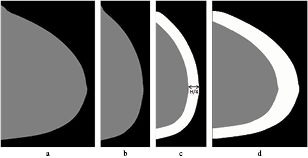
Figure 3. Image processing steps to determine the breast region that is in contact with the compression plate of a CC image. First, the segmented breast (a) is scaled to half width b), then an erosion and dilation with a circle structure element with a diameter of  is applied, leading to the band at the skin-line (c). That image is then rescaled to the original width (d).
Download figure:
Standard image High-resolution imageSince the description proposed by de Groot et al is for CC mammograms only, we adapted this approach for MLO views. We introduced a coordinate system in which the y-axis is defined by the pectoral muscle boundary, and the x-axis is perpendicular to the y-axis and goes through the nipple position. For each point within the breast segmentation, we determined the absolute angle ( ) between the x-axis and the line going through that point and the origin. Points that were closer to the skin-line than

were considered to belong to the region that is not in contact with the compression plates. Figure 4 shows a MLO mammogram with the coordinate system. Like in de Groot et al, we used H, obtained from the DICOM header, as thickness for the fully compressed breast region, and a thickness of  (average thickness of the peripheral zone) for the peripheral zone. The breast volume is the integral over the breast thickness over the breast area.
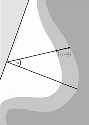
Figure 4. A schematic view of an MLO image and the differentiation into the fully compressed breast region (white) and the region where the breast is not in contact with the compression plates (gray). The coordinate system is based on the pectoral muscle segmentation and the estimated nipple position. For each point within the breast, the angle with the x-axis is determined (α). The two regions are defined by formula (6).
Download figure:
Standard image High-resolution image2.6. Segmentation of MR images
For evaluation of the methods we used breast MRI scans. First, the MRI scans were segmented into breast tissue and background. Each breast voxel was then labeled as fibroglandular tissue or fatty tissue. For most MRI's this was performed automatically with a previously developed method (Gubern-Mérida et al 2015). Some images were segmented manually. A manual segmentation was necessary, when the automatic segmentation was not accurate enough judged by a radiologist. Manual segmentations were performed by a trained researcher and were reviewed by a radiologist with expertise in breast MRI.
Manual segmentation was done as follows: in the axial view, in every 5–10 slices a contour was drawn around the breast outline using spline interpolation. Using these contours, the breast outline in the remaining slices was computed using a spline surface function to get the breast mask. These masks were checked and in case of an inaccurate segmentation, additional contours were drawn until the masks were accurate enough. Within the breast mask, contours for the segmentation into fibroglandular and fatty tissue were drawn in the same slices as the contours to segment the breast from background. These contours were extended to the whole breast with the method mentioned above. Within this fibroglandular tissue mask a threshold was applied to distinguish fibroglandular tissue from fatty tissue. Voxels outside the fibroglandular tissue mask but inside the breast mask were considered to be fatty. Segmentations were performed on bias field corrected images. The N4 bias field correction algorithm (Tustison et al 2010) was used.
3. Experiments
3.1. Material
We made use of 202 pairs of DM and MR examinations of 119 women recorded between December 2000 and December 2011 in the Radboudumc. MRI exams and mammograms were performed within two months of each other. All digital mammograms were acquired on GE Senographe systems using standard clinical settings with a non flexible compression paddle. For all examinations, a complete exam consisting of MLO and CC images of the left and right breast was available. We used the unprocessed (raw) data.
The MR examinations were performed on either a 1.5 or a 3 Tesla Siemens scanner (Magnetom Vision, Magnetom Avanto or Magnetom Trio), with a dedicated breast coil (CP Breast Array, Siemens, Erlangen, Germany). The segmentation of breast and fibroglandular tissue was performed on pre-contrast T1-weighted MR volumes without fat saturation. For 159 MRI examinations the automated segmentation was approved by a radiologist, 43 MRI's were segmented manually.
3.2. Comparison of mammography based fibroglandular tissue estimations to MRI data
The fibroglandular tissue volume estimations obtained with the three different reference values and the two combined approaches were compared to estimations based on MRI data. Results were averaged over MLO and CC views to obtain an estimate per breast. For an estimation per exam results were averaged over the left and right breast. Pearson's correlation coefficients and 95% confidence intervals (CI) were calculated using the statistical software package R. Because of the log-normal distribution of the data, correlation coefficients were computed after converting the measurements using the natural logarithm (Wang et al 2013, Gubern-Mérida et al 2014).
3.3. Comparison of breast volumes based on mammography and MRI
Mammographic breast volumes obtained with the two different geometrical approaches, the semi-circle model and the adaption of de Groot et al, were compared to breast volumes based on MRI data. Results were averaged over both mammographic views and over the left and right breast to obtain a single score for each exam. The MRI based breast volumes of the left and right breast were averaged as well. Pearson's correlation coefficients and 95% CI were calculated. Based on the performance of the two algorithms, we decided to proceed with one algorithm for further computations.
3.4. Evaluation of volumetric percent density estimations
The percent density estimations obtained with the three different reference values and the two combined estimates were compared to the estimations based on MRI data. Percent density is defined as fibroglandular tissue volume divided by breast volume. We made use of the breast volume estimations that are based on the work of de Groot et al In the original work of van Engeland the semi-circle model was used to obtain the breast volume. For comparison, percent density is given based on the fibroglandular tissue estimations with F1 and the breast volumes estimations of the semi-circle model as well. The estimations were again averaged over MLO and CC views to obtain an estimate per breast. To get an estimation for each exam, estimations were averaged over the left and right breast. Pearson's correlation coefficients and 95% CI were calculated.
3.5. Testing rotation invariance and effect of compression
To obtain a fatty tissue reference value with the dense tissue reference region approach we assume that the maximum dense tissue fraction (MDTF) in the direction of the mammographic compression (the direction of the x-ray beam) is the same as the MDTF in the image plane. This assumption is based on the idea that the MDTF does not depend on the direction of the measurement and is not affected by deformation of the breast due to compression. To investigate the validity of this idea we used the previously described data set of 202 MRI exams of 119 women. Additional, we included exams of 20 women who underwent MR guided biopsies and had breast density categorized as either BI-RADS 3 or 4. For each of these 20 women two MRI exams were available: an MRI recorded with the breast under compression in the MR guided biopsy procedure and a regular diagnostic MRI. The compression of the biopsied breast was always in the mediolateral direction. All MR images were manually segmented into fibroglandular tissue, fatty tissue and background.
To verify the rotation invariance of the MDTF measurements, we took samples in regular (uncompressed) MRI exams along lines in multiple directions in the coronal planes. Samples in each direction were taken on a regular grid in a square region of  , were the center of the square region projected to the center of the breast. By doing so, we prevented taking samples close to the pectoral boundary or near the breast edge. Samples had a cross section of
  . In each of these samples the fraction of dense tissue was computed from the segmented MRI. The MDTF was computed as a function of the projection angle by taking the maximum dense tissue fraction in the square region while rotating the breast. We took samples using 36 different angles, ranging between 0 and 175 degrees in steps of five degrees, simulating 36 different projection directions. The mean MDTF and the coefficient of variation when changing the projection angle were computed and displayed with a scatter plot. For this experiment we used both the set of 20 MRI's of uncompressed dense breasts and the 202 segmented MR images. In figure 5(a) a coronal slice of a MRI volume is given. The sample direction is craniocaudal.
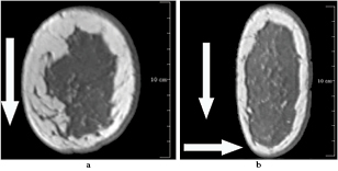
Figure 5. Two MRI exams of the same patient: (a) a coronal slice of an regular MRI volume, with an arrow indicating the craniocaudal direction in which the dense tissue fraction is determined, and (b) a coronal slice of an MRI volume recorded in a MR guided biopsy procedure, in which the dense tissue fraction was determined in two directions: mediolateral and craniocaudal as indicated by vertical and horizontal arrows, respectively.
Download figure:
Standard image High-resolution imageIn a second experiment we looked at the effect of compression using the exams of the patients who underwent MR-guided breast biopsies. We determined the maximum dense tissue fraction in the MRI's of the compressed breasts in two directions, one in the compression direction and one perpendicular to it, both along lines in parallel with the chest wall. These correspond to the directions in which we compute the maximum dense tissue fractions in the mammograms, with the difference that the MRI's are compressed in mediolateral directions while mammograms are compressed in the mediolateral oblique or craniocaudal direction. A visual example is shown in figure 5(b).
4. Results
4.1. Fibroglandular tissue volume
Figure 6 shows the results of the five methods for dense tissue volume estimation using MRI as a reference. The Pearson's correlation coefficients for the comparisons with MRI were 0.79, 0.80, 0.73, 0.83 and 0.86 when using F1, F2, F3, the combination of F1 and F2, and the combined estimates of F1–F3, respectively. In table 1 the correlation coefficients are given for the estimations averaged per breast and per exam.
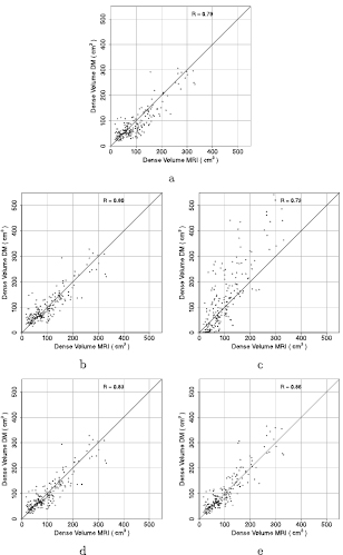
Figure 6. Comparison of fibroglandular tissue volume estimates per exam using the different reference values (a)–(c), the combination of F1 and F2 in (d) and the combination of the three methods in (e). The closed circles in the figures (a)–(c) belong to cases with a MDTF below 0.35, open circles have a MDTF above 0.35. In the figures (d)–(e), closed circles are used for exams that use the estimation of F1, while open circles are used when F2 (in (d)) or the combination of F2 and F3 (in (e)) is used.
Download figure:
Standard image High-resolution imageTable 1. Pearson's correlation coefficients with 95% CI for the five fibroglandular tissue volume estimations.
| Per breast | Per exam | |
|---|---|---|
| F1 | 0.77 (0.73–0.81) | 0.79 (0.73–0.84) |
| F2 | 0.78 (0.74–0.81) | 0.80 (0.74–0.84) |
| F3 | 0.71 (0.66–0.75) | 0.73 (0.66–0.79) |
| Combination F1 and F2 | 0.81 (0.78–0.84) | 0.83 (0.78–0.87) |
| Combination F1, F2 and F3 | 0.83 (0.80–0.86) | 0.86 (0.81–0.89) |
The parameters t, a and b that are needed to combine the results were obtained through cross validation. The optimal values for the parameters were determined in each fold and varied only a little. For both approaches, when combining F1 and F2, and when combining all three estimates, the optimal threshold was set to 0.35 (in four of the five folds). Therefore, the fibroglandular tissue volume as estimated with F1 is used if the MDTF < 0.35. The parameters a and b are needed when combing all three fibroglandular tissue volume estimates. In the majority of folds, the optimal values for a and b were 1.4 and −0.8 respectively. The MDTF is a first indication for the density. So in non-dense breasts the estimates as obtained with F1 are used while for dense breasts a combination of F2 and F3 works best.
4.2. Breast volume
Figure 7 shows results of the two breast volume estimation methods in comparison to MRI. Breast volume based on mammography has a linear relationship with the breast volume calculated from the MR images with both approaches. A Pearson's correlation coefficient of 0.96 (0.95–0.97 95%CI) was obtained for the semi-circle model and for the model in which the breast region that is in contact with the compression plates has a direction dependency. We decided to use the second approach, which is based on the idea of de Groot et al, for further calculations. This method appears to have less bias as the data points are closer to the identity line.
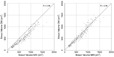
Figure 7. Comparisons of breast volume obtained with MRI and mammography, averaged per examination. On the left side are the estimations with the semi-circle model, while on the right side are the estimates based on the idea of de Groot et al, where the definition of the fully compressed breast region has a direction dependency.
Download figure:
Standard image High-resolution image4.3. Volumetric breast density estimation
Figure 8 shows the comparison between volumetric percent density estimates from DM and MRI. The Pearson's correlation coefficients between the volumetric percent density estimations per study were 0.86, 0.89, 0.74, 0.87 and 0.90 when using F1, F2, F3, the combination of F1 and F2 and the combination of F1 − F3, respectively. When using the fibroglandular tissue estimations with F1 and the semi-circle model for the breast volume a correlation of 0.88 was found. Pearson's correlation coefficients with 95% CI are shown in table 2 for comparisons per breast and per exam.
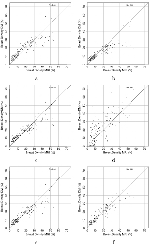
Figure 8. Comparison of percent density estimations per exam. In (a) the fibroglandular tissue estimation of F1 is combined with the breast volume obtained of the semi-circle model. Results are therefore comparable to the original work of van Engeland. For the results in (b)–(f) the breast volume as obtained from the second algorithm was used. The graphs (b)–(d) belong to the three different reference values F1, F2 and F3 respectively. The results in (e) and (f) are from the combination of the methods with in (e) the combination of F1 and F2 and in (f) the combination of all three fibroglandular tissue estimations.
Download figure:
Standard image High-resolution imageTable 2. Pearson's correlation coefficients with 95% CI for the six volumetric density estimations. When not indicated the breast volume as obtained with de Groot et al was used.
| Per breast | Per exam | |
|---|---|---|
| F1 With semi-circle model | 0.87 (0.84–0.89) | 0.88 (0.84–0.91) |
| F1 | 0.84 (0.81–0.87) | 0.86 (0.82–0.89) |
| F2 | 0.87 (0.85–0.89) | 0.89 (0.86–0.91) |
| F3 | 0.73 (0.68–0.77) | 0.74 (0.67–0.80) |
| Combination F1 and F2 | 0.87 (0.84–0.89) | 0.89 (0.85–0.91) |
| Combination F1, F2 and F3 | 0.89 (0.87–0.91) | 0.90 (0.88–0.93) |
4.4. Rotation invariance and the effect of breast deformation
We determined MDTF values for different projection angles in the MR images of 20 dense breasts and the 202 segmented MR volumes. With a rotation interval of 5 degrees, this yielded to MDTFs of 36 different angles. The mean MDTF ranged between 0.11 and 0.95 and the coefficient of variation of the measurements ranged between 0.01 and 0.54. In figure 9(a) a scatter plot of the mean MDTF and the coefficient of variation is shown. We see that the coefficient of variation decreases with an increase of the mean MDTF. The low coefficient of variation of dense breasts (high mean MDTF), indicates that the MDTF is almost direction invariant in extremely dense breasts. On the other hand, the coefficient of variation is larger of small mean  . As the MDTF is a first indication for the breast density, we can see that the idea of direction invariance is violated in non-dense breasts. Hence, it is no surprise that the MDTF used to estimate F3 becomes unreliable, resulting in unrealistic low dense volume measurements (see also figure 6(c)).

Figure 9. Left: mean and coefficient of variation of the 36 MDTF measurements of the MR images of the 20 uncompressed breasts (closed circle) scored as BI-RADS density 3 or 4, and the 202 segmented MR images (open circle). Right: maximum dense tissue fraction measured in MRI's with compression of the breast in mediolateral direction. The dense tissue fractions in the direction of the compression are compared to the perpendicular direction.
Download figure:
Standard image High-resolution image
The comparison of the maximum dense tissue fractions measured in coronal planes of the compressed breast MRI's is shown in figure 9(b). Results obtained in the mediolateral direction, the direction of the compression, are on the vertical axis, while results of the craniocaudal direction are plotted horizontally. It can be observed that the maximum dense tissue fraction (MDTF) in the two directions are quite similar, which supports the validity of our approach.
5. Discussion
Accurate and reliable breast density measurements are needed when using density for stratification or breast cancer risk analysis. In this study, we experimented with the use of different internal reference values for calibration of a widely used volumetric breast density quantification method. We used reference values of pure fatty pixels using two different breast interior definitions and also proposed a novel approach, which employs the densest region in a mammogram as a reference. Hybrid approaches to obtain robust estimates in fatty and dense breasts, which combines breast density estimates, are also proposed.
We estimated the reference value of purely fatty tissue based on the pixel value distribution in the breast interior. The two reference values F1 and F2 use different definitions of the breast interior. The third reference value F3 was determined based on a pixel value representative for the densest region in the mammogram. When comparing volumetric percent density based on mammography to MRI data for each exam, Pearson's correlation coefficients of 0.86, 0.89 and 0.74 were found when using F1, F2 and F3, respectively, when using de Groot to obtain the breast volume estimate.
Results show that the individual performance of F1 and F2 is much better than the one of F3. Therefore, it might be questionable whether F3 adds a lot to the performance of a hybrid approach. However, in our experiments best results were obtained when combining all three estimations (Pearson's correlation 0.90). This can be explained by the fact that different breast density patterns require different approaches. Compared to the original method, a clear improvement is visible in the scatter plots when comparing the results to that of the combined approach (figure 8), in particular for dense breasts. The combination of results of F1 and F2 yielded a correlation coefficient of 0.89. Though the difference in correlation coefficient between the two hybrid methods is small, substantial differences are visible between the two scatter plots for dense breasts. This confirms that a new approach is necessary to deal with extremely dense breasts. The difference in correlation found in our study is not large, we expect larger differences when more cases with dense breasts would be included in the study set. An analysis with only dense breasts might be carried out in the future.
The novel method based on using the densest region in a mammogram as a reference relies heavily on the assumption that the maximum dense tissue fraction (MDTF) does not strongly depend on the projection angle and the compression. We tested the assumption that the MDTF is rotation invariant in planes in parallel to the chest wall using MRI exams with segmentations of fibroglandular tissue. For 424 breasts the mean MDTF computed in 36 directions and the coefficient of variation were determined. As expected, the coefficient of variation decreases with an increase of MDTF. For extremely dense breasts, the coefficient of variation becomes as low as 0.05. This indicates that the method we propose is a feasible alternative to methods relying on a fatty tissue reference region when breasts are dense. It should also be noted that random errors due to variation of the direction in which the dense tissue fraction is measured are reduced because in mammography we combine four measurements, the MLO and CC projections of both breasts, into a single density measurement. For non-dense breasts the method cannot be used because the assumption of rotation invariance is violated.
A second assumption was made that the MDTF in the direction of the compression is comparable to the MDTF in a direction perpendicular to the compression force. Results in figure 9(b) suggest that this is true in good approximation. For a moderately compressed breast, as obtained in MRI guided biopsy procedures, the MDTF in both directions are comparable to each other.
Breast MRI scans were used for validation in which fibroglandular tissue, fatty tissue, and background were segmented. While some of these segmentations were obtained manually, most were automatically generated. That we used a mix of two segmentation methods may be regarded as a drawback since it could introduce an additional source of error. However, we observed that the range of volumetric breast density estimates of the manual segmented MRI's is comparable to the range of estimations obtained with the automatic segmented MR images (1.7–51.2% compared to 2.4–56.6%). Therefore, we believe that the manually segmented cases were not systematically denser of less dense than the automatically segmented cases.
In this study, we also investigated two different breast volume computation methods. Accurate estimation of breast volume is important because this is needed to obtain volumetric percent density. We found that a recently proposed method which extends the semi-circle model of the breast edge shape leads to visually improved results when MRI is used as a reference. In this paper we adapted the method in such a way that it can be applied to both MLO and CC views. Both approaches resulted in a high correlation coefficient when compared to the breast volumes estimations computed from MRI data. However, the methods have a tendency to underestimate breast volume, but the bias is less prominent in the new method. This can be seen as well in figure 8(a) were percent breast density is overestimated as the breast volume of the semi-circle model is underestimated. Some underestimation might be expected though, since the field of view of both imaging techniques is different. The imaged part of the breast in a mammogram relies strongly on the positioning of the patient. With MRI, the complete breasts and parts of the thorax are always imaged.
The algorithm of de Groot to estimate the breast volume defines a contact surface of the breast and the compression paddle that is slightly different from the one we used for defining the breast interior region for reference value F2. Though we could have used this, we decided not to use this alternative interior region definition. The reason is that we noted that due to inclusion of more pixels at the peripheral region border there was a high risk of including poorly compressed tissue regions close to the chest wall, especially in the MLO views. Inclusion of such regions might easily lead to large errors in the dense tissue estimation.
A limitation is that the study makes use of mammograms obtained at a single site with a single vendor. The studies of Wang et al (2013) and Gubern-Mérida et al (2014) have, however, shown that the breast density can be reliable estimated with the reference method across vendors and that there is a problem with extremely dense breasts independent of the manufacturer of the mammographic system. Gubern-Mérida made use of images obtained with GE equipment, while Wang et al used images acquired on Hologic systems. Hence, we do not expect problems with images from other vendors than GE.
In this study we proposed a novel approach to improve breast density estimation in dense breasts. By including the densest region in a mammogram as a reference and by adapting the region in which a fatty tissue reference region is selected we achieved better results compared to the existing approach. Results demonstrate that it remains crucial to find a good reference value for fatty tissue in order to get a reliable breast density estimate. Different fibroglandular tissue patterns within the breast require different techniques to estimate the fibroglandular tissue volume and percent volumetric density.
Acknowledgments
The research leading to these results has received funding from the European Union's Seventh Framework Programme FP7 under grant agreement no 306088.