
Abstract
Heat transfer is a phenomenon well known from everyday life. It is intuitively connected to the properties of materials, that is, to the physics concept of thermal conductivity relevant for cooking or maintaining the constant temperature in rooms, even without being familiar to the underlying physics. However, measurement of thermal conductivity is usually demanding, but here we present a simple, quick, and almost hands-on method that yields quite accurate values for thermal conductivity of insulating and semi-insulating materials, appropriate for a classroom setting.
Export citation and abstract BibTeX RIS

Content from this work may be used under the terms of the Creative Commons Attribution 4.0 licence. Any further distribution of this work must maintain attribution to the author(s) and the title of the work, journal citation and DOI.
1. Introduction
Heat transfer is a well-known everyday phenomenon. People intuitively connect it to the properties of materials, for example, to cooking or insulation of houses, even without being familiar with the underlying physics. Heat transfer strongly depends on the material, characterized by its coefficient of thermal conductivity  . In the school setting, it is unfortunately rather demanding to find its approximate value, because experiments usually require rather sophisticated equipment not available in schools [1–4]. An additional problem is the heat transfer due to convection, which is difficult to eliminate, or at least to control and estimate [3, 5, 6]. Several experiments, however, provide experience and scaffold the concept to students on the semi-quantitative level [7], but teachers are often forced to limit the consideration of thermal conductivity to comparison of materials with significantly different conductive properties, such as metals and polystyrene. We believe that this paper bridges this gap, as we present a simple, quick, and almost hands-on method for measuring the thermal conductivity of insulating and semi-insulating materials, appropriate for a classroom setting.
The suggested measurement of thermal conductivity is based on measuring the temperature's dependence on time of a cooling water immersed in a mixture of ice and water for a relatively short period of time. The setup for the suggested experiment is very simple and straightforward. For the analysis of the measurements we suggest a simple trick for reorganization of the measured data, which straightforwardly leads to the coefficient of thermal conductivity. The method gives relatively accurate thermal conductivities for poor conductors and for conductors that have smaller thermal conductivity than still water, which is used as a cooling medium. The method has some limitations, however. Although the setup eliminates the influence of convection and radiation, it is still not appropriate for very good conductors like metals. Possible reasons for this limitation are discussed in the paper as well.
The method is actually a modernized and simplified version of the approach presented more than two decades ago [2]. The experimental setup of this method is much simpler and easier to assemble. The estimation of the transferred heat, which was based on determination of the mass of melted ice [2] is replaced by a continuous measurement of the temperature, and the analysis of the measured data can be simplified for time periods during which the measured medium cools down for a few tens of degrees only.
2. Thermal conductivity and cooling of water
Let us consider a closed container with conductive walls filled with water. The walls are made of a material with the coefficient of thermal conductivity λ having a thickness  , and the surface area of the container
  . The water in the container has a mass
  and the specific heat
  . Initially, the container is filled with hot water close to the boiling point. The container with the water having the initial temperature
  is quickly immersed into a large reservoir with a mixture of water and ice having temperature
  . Temperature of the water in the container
  is measured for a few minutes. For described circumstances, the interfaces between the container and the water in its interior and between the container and the water-ice mixture in the reservoir have the same temperature as the liquid in contact, therefore the transfer of heat by radiation is negligible (see also supplementary materials 1, available online (stacks.iop.org/PhysED/55/045004/mmedia)). In addition, the liquid inside the container is slightly mixed, which ensures equal temperatures of the water near the walls and in the middle of container. The convection in the reservoir with the mixture of water and ice is negligible. Therefore, to describe the temperature dependence of the water in the container on time
  , only the analysis of heat conduction through the walls of the container satisfies.
Let us define the temperature difference between the time dependent water temperature and the (constant) reservoir temperature as θ, i.e.  . The temperature of water in the container decreases due to the heat transfer through the walls of container:
which yields the time dependence of the temperature difference as

Here θ0 is the initial temperature difference  The characteristic time, τ, is the time when the temperature difference decreases to 1/e (approximately 37%) of the initial value. Equations (1) and (2) are classical expressions students meet at exercises in introductory physics courses. For times smaller than characteristic times Δt <
 , the dependence (2) can be linearized, which leads to the same expression as in (1) in a non-differential form. In the time Δt the temperature of water in the container changes for
  due to the transfer of heat to the container. The transfer of heat is a consequence of temperature difference
 between the water in the container and in the reservoir. The linearized equation (1) becomes
Let us use a shorter notation for the time dependent temperature difference  in continuation, to further simplify the expression (3) to
Introducing the ratio between the magnitude of the temperature change and the temperature difference as  and see that it depends linearly on time
with a gradient  , allows for straightforward determination of thermal conductivity λ.
3. The experimental setup
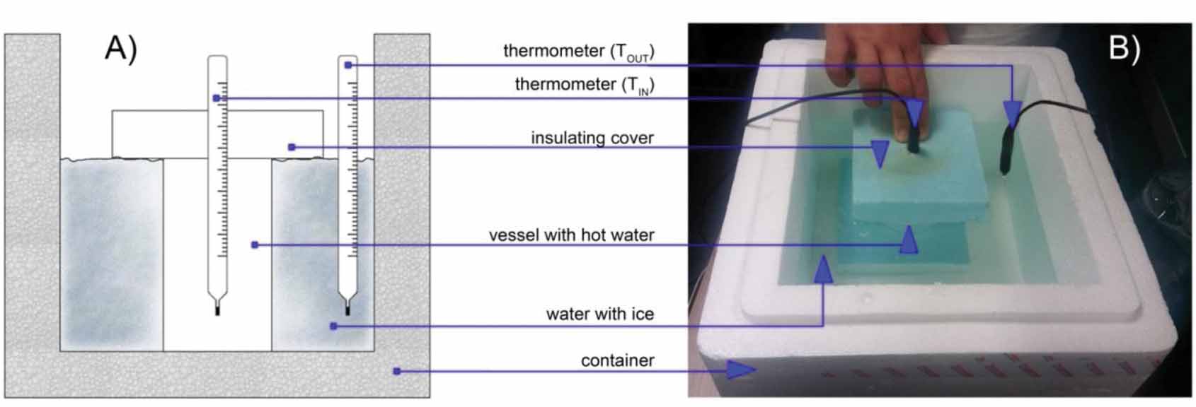
The here-presented experimental setup consisted of a reservoir with inner dimensions 24 cm times 25 cm and the height about 20 cm containing several liters (between 5 and 7 in figure 1(b)) of water with crushed ice, in ratio 1:1 approximately. For the setup, a polystyrene box for transport of cooled vegetables was used. As containers for the warm water, we used cups from different materials. Each cup was filled with hot water directly out of the kettle, it was covered by a thick polystyrene cover, and the thermometer connected to Vernier interface was inserted into the hole in the cover. The cup prepared in this way was immersed into the reservoir as shown on the schematic drawing in figure 1(a). The whole procedure, from pouring the almost boiling water to the cup to inserting the cup into the reservoir, should be as quick as possible in order to achieve the highest possible temperature difference between the water in the cup and in the reservoir. The temperature of the water in the cup was measured by a thermometer for the duration of a few minutes. The temperature of the mixture of ice and water in the reservoir was also controlled and it was slightly stirred once per minute to prevent local increases of the temperature close to the cup's walls.
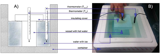
Figure 1. (a) The sketch of the experimental setup. (b) The actual setup.
Download figure:
Standard image High-resolution image4. The measured coefficients of the thermal conductivity
To measure the thermal conductivity of different materials, the time dependent temperature of the cooling water in five different cups made of different materials was measured. The cups used for this experiment were made of polystyrene, wood, plastic, porcelain, and stainless steel. Properties of the cups, together with calculated characteristic times  from the thermal conductivities available in literature [8] are presented in table 1. Temperature was measured by the Coach6 system external thermometer with an accuracy of 0,1 °C in 1 s intervals. Diameters were obtained by a caliper and for the specific heat of water, the value 4 200 J kg−1 K−1 was used. More properties of cups are given in the supplementary material 2.
Table 1. The cups and their properties with calculated characteristic times  .
.
| Polystyrene | Wood | Plastic | Porcelain | Metal (stainless steel) | |
|---|---|---|---|---|---|
| Photo | |||||
| S (cm2) | 213 ± 8 | 196 ± 7 | 307 ± 9 | 203 ± 7 | 230 ± 8 |
| d (mm) | 2.0 ± 0.1 | 5.0 ± 0.1 | 2.0 ± 0.1 | 4.9 ± 0.1 | 0.6 ± 0.1 |
| mw(g) | 260 ± 10 | 270 ± 10 | 653 ± 10 | 348 ± 10 | 584 ± 10 |
|
λ (W m−1 K−1) | 0.03 | 0.16 | 0.3 | 1.5 | 16 |
 (s) (s) | 3400 ± 430 | 1807 ± 168 | 596 ± 56 | 240 ± 20 | 4.0 ± 0.9 |
a The thermal coefficient of wood depends on a type of wood and the direction with respect to fibers and it varies from 0.12 to 0.17. b The thermal coefficient of plastic depends on the type of polymers and the temperature and it varies from 0.17 to 0.50, type of plastic in the mug was unknown. c The values for the thermal conductivity were taken from [8]. Additional data are available in supplementary material 2 online.
Figure 2(a) shows the temperature dependence of water in the studied cups during cooling. Figure 2(b) shows the time dependence of the ratio  calculated from the measured temperatures for a time period of 500 s (polystyrene, wood, plastic) or of 200 s (porcelain, steel). The coefficient of the linear fit was extracted for each material and a thermal conductivity was calculated from the fitted slope (5). Results are presented in table 2.
Table 2. Results of linear regression to acquired data and calculated thermal conductivity coefficients. Theoretical values retrieved from [8]. Uncertainties of experimental values are between 20% and 30% in spite the simplicity of the method.
| Polystyrene | Wood | Plastic | Porcelain | Metal (stainless steel) | ||
|---|---|---|---|---|---|---|
Slope  (
( = 0.02) = 0.02) | 0.00042 | 0.00053 | 0.00143 | 0.0047 | 0.014 | |
Characteristic time  ( ( = 0.02) = 0.02) | 2380 | 1890 | 700 | 212 | 71.5 | |
 (W m−1W K−1) (W m−1W K−1) | Literature | 0.03 | 0.12–0.17 | 0.17–0.50 | 1.5 | 16 |
| Exp. value | 0.04 ± 0.01 | 0.15 ± 0.03 | 0.25 ± 0.05 | 1.57 ± 0.30 | 4.4 ± 1.4 | |

Figure 2. (a) Temperature dependence of the water in the cup immersed in the mixture of water and ice in the analyzed range. (b) The time dependent ratio  calculated from the measured temperatures for the studied cups. The data is presented in two separate graphs with different time and ratio scales as the slopes of r(t) for porcelain and steel are much larger. Measurements presented by open symbols in (a) are not included in the second graph in (b).
Download figure:
Standard image High-resolution image
The obtained values of thermal conductivity are consistent with the ones given in literature11 for all used materials except for steel. Therefore, one can conclude that for insulators like polystyrene or weak insulators like wood, plastic, or porcelain, the method is quite reliable and accurate. However, comparing the measured thermal conductivity for steel and its value in literature, one can observe a severe discrepancy. How can this result be interpreted? The calculated characteristic time for a steel cup is 4 s, but the one measured according to the method is more than 70 s. Even more, the time dependence of the ratio  within the measured characteristic time span is almost linear, suggesting that also the cooling behavior is very similar to poor and weak conductors and, therefore, the method could be used. But, it is far from true. We investigated this phenomenon into more detail. We measured several 'cups', that is, empty cans from various metals like cola can and cans previously filled with conserved vegetables made of different metals. This discrepancy occurred for each good thermal conductor. We speculate that the origin of this discrepancy is the following. Cans from good thermal conductors transfer the heat very efficiently through the walls of the can. As the water in the can close to the walls cools almost uniformly, the convection is probably small. One therefore cannot consider that the whole water in the can cools uniformly, but the transfer of heat to the water in the interior of the cup has to be considered as well. The thermal conductivity of water without a convection is 0.6065 W m−1 K−1 which is more than ten times less than that of steel. Layers of water close to the walls with intensive heat transfer actually act like an inner 'insulation' in the cup. If the data for good conductors are analyzed in the same way as for poor and weak conductors, what is actually measured is an effective thermal conductivity that includes the layers of water close to the walls. This explanation is further supported by closer examination of the initial time dependence of the ratio
  of the wooden cup. It is not linear at the beginning of the measurement. Why not? Wood is a relatively good insulator but also has a significant thermal capacity. Therefore, after the wooden cup with the hot water was set into the reservoir, the cup's walls started to cool. The conduction of heat could not have been described by the simple equation given in (2) as long as the temperature profile in the wooden walls of the container was not linear.
The presented methodology is therefore limited to materials with the thermal conductivity comparable or lower than water, which was already mentioned earlier [5]. As the thermal conductivity is calculated from the slope of the  one remains on the safe side if the water temperature does not change more than 10 °C to 20 °C and the temperature difference to the reservoir is still above 50 °C. To avoid unexpected transition phenomena like the time needed for warming or cooling the cups, it is advised to start the measurement about 10–20 s after the cup is immersed to the reservoir.
In spite of the simplicity, the method gives surprisingly accurate thermal conductivities of weak and good thermal insulators. Because the water temperature in the cup for materials that could be measured by this method does not change dramatically, the computerized measurement as was used here is not crucial. The temperature could also be measured manually still resulting in relatively accurate values for thermal conductivities.
5. Conclusions
We presented a simple and efficient method for a relatively fast measurement of thermal conductivity appropriate for insulators or semi-insulators, that is, poor conductors. The presented setup could be used as a demonstration experiment in the classroom setting or as a rather simple and straightforward laboratory experiment. Simplicity, intuitiveness, and the low cost of the experiment are features that make the proposed experiment an excellent support to introduction of thermal conductivity. Moreover, the suggested method for the measurement of thermal conductivity links together the heat flow and its consequences, which additionally develops the awareness of processes that are common reasons for changes of temperatures and their dynamics. It also shows that the physical properties of different materials are not just abstract numbers calculated by engineers but real features, the consequences of which one can observe and measure their values.
Biographies
Mojca Ćepič teaches future teacher of physics at University of Ljubljana, Faculty of Educations, both, theoretical subjects and methodology of teaching physics. Her research is focused on two fields: on physics education and on theoretical soft matter physics, more precisely on polar smectic liquid crystals. She is mostly occupied with designing and testing of simplified experiments, which introduce contemporary physics results to pre-university education.
Daniel Dziob is completing a doctorate in biophysics at the Faculty of Physics, Astronomy and Applied Computer Sciences, Jagiellonian University, Krakow. His research focuses on two fields: physics education and cell migration. He also works and teaches biophysics for medical students at the Jagiellonia University Medical College. As a hobby, he teaches physics to high school students, hikes and annoys his friends and collaborators with new ideas.