Estimation of solid-state sintering and material parameters using phase-field modeling and ensemble four-dimensional variational method

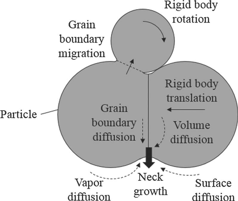
Figure 1 shows the multiple physical phenomena that occur during solid-state sintering. These types of microstructural evolution including neck growth, grain boundary migration, and grain growth occur by four types of atomic diffusion: volume, vapor, surface, and grain boundary diffusion. In addition, over-saturation of vacancies at grain boundaries caused by the atomic diffusions leads to rigid body motion of sintered particles [19]. The rigid body motion consisting of particle translation and rotation drives the densification of the sintered material. To describe these sintering phenomena, we employ the PF model proposed by Wang [19], which can simultaneously analyze both microstructural evolution and densification by calculating the four types of diffusion and the particle rigid body motion.

Zoom In Zoom Out Reset image size

To simulate the microstructural evolution during solid-state sintering, we define two types of PF variables: the density field, ρ, and orientation field, η_i (i = 1, 2, 3, ..., N, where N is the total number of particles). Figure 2 shows the distributions of ρ and η_i employed to describe two sintered particles. ρ represents the probability of particle existence, while η_i identifies the individual particle geometry. Both ρ and η_i change smoothly from 0 to 1 on the surface and in the grain boundary regions.

Zoom In Zoom Out Reset image size

The total free energy F is defined as

$$\begin{equation}F={\int }_{V}\left\{{f}_{ \mathrm{b}\mathrm{u}\mathrm{l}\mathrm{k}}\left(\rho ,{\eta }_{i}\right)+\frac{{\kappa }_{\rho }}{2}{\left\vert \nabla \rho \right\vert }^{2}+\sum\limits _{i}^{N}\frac{{\kappa }_{\eta }}{2}{\left\vert \nabla {\eta }_{i}\right\vert }^{2}\right\}\mathrm{d}V,\end{equation} \tag{ 1 }$$

where f_bulk(ρ, η_i ) is the bulk chemical free energy density. The second and third terms are the gradient energy densities. κ_ρ and κ_η are the gradient energy coefficients [21, 22]. The function f_bulk(ρ, η_i ) is given by [19–23]

$$\begin{equation}{f}_{ \mathrm{b}\mathrm{u}\mathrm{l}\mathrm{k}}=A{\rho }^{2}{\left(1-\rho \right)}^{2}+B\left[{\rho }^{2}+6\left(1-\rho \right)\sum\limits _{i}^{N}{\eta }_{i}^{2}-4\left(2-\rho \right)\sum\limits _{i}^{N}{\eta }_{i}^{3}+3{\left(\sum\limits _{i}^{N}{\eta }_{i}^{2}\right)}^{2}\right],\end{equation} \tag{ 2 }$$

where A and B are constants [21–23].

Because we assume that mass conservation is satisfied during sintering, the integrated particle density remains constant. Therefore, ρ is defined as a conserved variable. The time evolution of ρ can be derived from the Cahn–Hilliard equation [58]:

$$\begin{equation}\frac{\partial \rho }{\partial t}=\nabla \cdot \left\{{M}_{\rho }\nabla \left(\frac{\partial {f}_{ \mathrm{b}\mathrm{u}\mathrm{l}\mathrm{k}}}{\partial \rho }-{\kappa }_{\rho }{\nabla }^{2}\rho \right)\right\}.\end{equation} \tag{ 3 }$$

Here, M_ρ is the diffusion mobility, which can be written as [21]

$$\begin{equation}{M}_{\rho }={M}_{\mathrm{v}\mathrm{o}\mathrm{l}}q\left(\rho \right)+{M}_{\mathrm{v}\mathrm{a}\mathrm{p}}\left\{1-q\left(\rho \right)\right\}+{M}_{\mathrm{s}\mathrm{u}\mathrm{r}\mathrm{f}}{\rho }^{2}{\left(1-\rho \right)}^{2}+{M}_{\mathrm{g}\mathrm{b}}\sum\limits _{i}^{N}\sum\limits _{j\ne i}^{N}{\eta }_{i}{\eta }_{j},\end{equation} \tag{ 4 }$$

where M_vol, M_vap, M_surf, and M_gb are the atomic mobilities related to the bulk, vapor, surface, and grain boundary diffusion coefficients, respectively. q(ρ) is an interpolation function given by q(ρ) = ρ³(10 − 15ρ + 6ρ²). The mobilities are defined as M_X = V_m D_X /RT, where X (X = vol, vap, surf, gb) expresses each diffusion path [21, 59], R is the gas constant, T is the absolute temperature, and V_m is the molar volume. D_X is the diffusion coefficient for each diffusion path.

To simulate the rigid body motion of the particles during sintering, an advection term is added to the right-hand side of equation (3):

$$\begin{equation}\frac{\partial \rho }{\partial t}=\nabla \cdot \left\{{M}_{\rho }\nabla \left(\frac{\partial {f}_{ \mathrm{b}\mathrm{u}\mathrm{l}\mathrm{k}}}{\partial \rho }-{\kappa }_{\rho }{\nabla }^{2}\rho \right)-\rho \sum\limits _{i}^{N}{\boldsymbol{v}}_{\mathrm{a}\mathrm{d}\mathrm{v},i}\right\},\end{equation} \tag{ 5 }$$

where v _adv,i is the advection velocity of the ith particle (i = 1, 2, 3, ..., N). Because the rigid body motion of a particle consists of translation and rotation, v _adv,i is given by

$$\begin{equation}{\boldsymbol{v}}_{\mathrm{a}\mathrm{d}\mathrm{v},i}={\boldsymbol{v}}_{\mathrm{t}\mathrm{r},i}+{\boldsymbol{v}}_{\mathrm{r}\mathrm{o},i},\end{equation} \tag{ 6 }$$

where v _tr,i and v _ro,i are the translational and rotational velocities of the ith particle, respectively. v _tr,i is given by

$$\begin{equation}{\boldsymbol{v}}_{\mathrm{t}\mathrm{r},i}=\frac{{m}_{\mathrm{t}\mathrm{r}}}{{V}_{i}}{\boldsymbol{F}}_{i}{\eta }_{i},\end{equation} \tag{ 7 }$$

where m_tr is the translational mobility of the particle, V_i is the volume of the ith particle, and F _i is the force acting on the ith particle. F _i is given by

$$\begin{equation}{\boldsymbol{F}}_{i}={\int }_{V}\mathrm{d}{\mathbf{F}}_{i},\end{equation} \tag{ 8 }$$

where d F _i is the local force density that is defined as

$$\begin{equation}\mathrm{d}{\boldsymbol{F}}_{i}={k}_{\mathrm{s}\mathrm{t}}\sum\limits _{j\ne i}^{N}\left(\rho -{\rho }_{0}\right)\left\langle {\eta }_{i}{\eta }_{j}\right\rangle \left[\nabla {\eta }_{i}-\nabla {\eta }_{j}\right]{\mathrm{d}}^{3}r.\end{equation} \tag{ 9 }$$

The coefficient k_st in equation (9) is a stiffness constant related to the magnitude of the force caused by the over-saturated vacancies at grain boundaries. ρ₀ is an equilibrium value of ρ at grain boundaries and is set to slightly smaller than ρ = 1 to mimic the over-saturation of vacancies. The operation ⟨η_i η_j ⟩ is defined as

$$\begin{equation}\left\langle {\eta }_{i}{\eta }_{j}\right\rangle =\left\{\begin{gathered}1\quad \left({\eta }_{i}{\eta }_{j}{\geqslant}c\right)\\ 0\quad \left({\eta }_{i}{\eta }_{j}{< }c\right)\end{gathered}\right.,\end{equation} \tag{ 10 }$$

where c is a threshold value for identifying grain boundary regions. The rotational velocities of the ith particle, v _ro,i , in equation (6) is given by

$$\begin{equation}{\boldsymbol{v}}_{\mathrm{r}\mathrm{o},i}=\frac{{m}_{\mathrm{r}\mathrm{o}}}{{V}_{i}}{\boldsymbol{T}}_{i}{\times}\left[\boldsymbol{r}-{\boldsymbol{r}}_{c,i}\right]{\eta }_{i},\end{equation} \tag{ 11 }$$

where m_ro is the rotation mobility of the particle. r is the position vector and r _c,i indicates the center of the ith particle. The symbol '×' denotes the vector product operator. T _i is the torque acting on the ith particle and is given by

$$\begin{equation}{\boldsymbol{T}}_{i}={\int }_{V}\left[\boldsymbol{r}-{\boldsymbol{r}}_{c,i}\right]{\times}\mathrm{d}{\boldsymbol{F}}_{i}.\end{equation} \tag{ 12 }$$

During sintering, the shape of each particle changes due to grain growth and grain boundary migration. Thus, the orientation field η_i is defined as a non-conserved variable. The time evolution of η_i can be defined by adding an activation term to the Allen–Cahn equation [60]:

$$\begin{equation}\frac{\partial {\eta }_{i}}{\partial t}=-{M}_{\eta }\left(\frac{\partial {f}_{ \mathrm{b}\mathrm{u}\mathrm{l}\mathrm{k}}}{\partial {\eta }_{i}}-{\kappa }_{\eta }{\nabla }^{2}{\eta }_{i}\right)-\nabla \cdot \left({\eta }_{i}{\boldsymbol{v}}_{\mathrm{a}\mathrm{d}\mathrm{v},i}\right),\end{equation} \tag{ 13 }$$

where M_η is the PF model parameter that is correlated to the mobility of grain boundary migration.

The time evolution equations of ρ and η_i given by equations (5) and (13), respectively, are solved by the first-order Euler finite difference method for time integration and the second-order central finite difference method for spatial discretization.

A DA based on Bayesian inference requires the definition of a state vector and an observational vector. The state vector contains all state variables used in the numerical model, while the observation vector consists of experimental or observational data.

The vectors x _t and y _t are defined as the state and the observation vector at time t (0 ⩽ t ⩽ t_end), respectively. In the present study, x _t contains not only the state variables but also the unknown material parameters to be estimated, and is therefore called the augmented state vector. Both x _t and y _t are assumed to have noise, specifically, system noise and observational noise, respectively. The system noise represents the error contained in the simulation results due to numerical calculation errors, simulation model imperfections, material parameter uncertainty, etc. The observational noise describes the error of the observational data. The noises are independent and follow a Gaussian distribution [42]. Under the above assumptions, x _t and y _t at arbitrary times are treated as stochastic variables that follow the Gaussian PDF. Using x _t and y _t , the 4DVar and En4DVar are formulized as described below.

En4DVar is a DA method based on 4DVar. In the 4DVar method [41, 42], the first estimated initial state vector, ${\boldsymbol{x}}_{0}^{b}$, called the background state vector, is defined. A conditional PDF, which indicates the probability density of ${\boldsymbol{x}}_{0}^{b}$ when x ₀ is given, is expressed using a Gaussian distribution:

$$\begin{equation}p\left({\boldsymbol{x}}_{0}^{b}\vert {\boldsymbol{x}}_{0}\right)=\frac{1}{\sqrt{{\left(2\pi \right)}^{l}\left\vert \boldsymbol{B}\right\vert }}\enspace \mathrm{exp}\left[-\frac{1}{2}{\left({\boldsymbol{x}}_{0}-{\boldsymbol{x}}_{0}^{b}\right)}^{\mathrm{T}}{\boldsymbol{B}}^{-1}\left({\boldsymbol{x}}_{0}-{\boldsymbol{x}}_{0}^{b}\right)\right],\end{equation} \tag{ 14 }$$

where l is the number of state vector dimensions and B is a covariance matrix of the PDF p(${\boldsymbol{x}}_{0}^{b}$| x ₀), which is called the background error covariance matrix in 4DVar. The superscript T denotes a transposition of a matrix. A conditional PDF at time t, which indicates the probability density of the observation vector y _t when state vector x _t is given, is also represented using a Gaussian distribution:

$$\begin{equation}p\left({\boldsymbol{y}}_{t}\vert {\boldsymbol{x}}_{t}\right)=\frac{1}{\sqrt{{\left(2\pi \right)}^{m}\left\vert {\boldsymbol{R}}_{t}\right\vert }}\enspace \mathrm{exp}\left[-\frac{1}{2}{\left({H}_{t}\left({\boldsymbol{x}}_{t}\right)-{\boldsymbol{y}}_{t}\right)}^{\mathrm{T}}{\boldsymbol{R}}_{t}^{-1}\left({H}_{t}\left({\boldsymbol{x}}_{t}\right)-{\boldsymbol{y}}_{t}\right)\right],\end{equation} \tag{ 15 }$$

where m is the number of observation vector dimensions and H_t is an observational operator that extracts quantities comparable to y _t from x _t . R _t is the observation error covariance matrix of the PDF p( y _t | x _t ). In this study, R _t is defined as R _t = σ² I , where I is an identity matrix whose dimension is m × m. σ denotes a parameter which determines the magnitude of the observational noise that mimics an observational error.

Because the time evolution of x _t can be calculated by PF simulation, x _t is expressed as

$$\begin{equation}{\boldsymbol{x}}_{t}=M\left({\boldsymbol{x}}_{t-1}\right)={M}^{t}\left({\boldsymbol{x}}_{0}\right),\end{equation} \tag{ 16 }$$

where M is a model operator, which corresponds to the PF model presented in section 2.1. M^t denotes that M acts on x ₀ repeatedly until time t. Therefore, M^t ( x ₀) is equivalent to performing a numerical simulation of solid-state sintering using the PF model. According to equation (16), H_t is written by defining another observational operator, Ĥ_t :

$$\begin{equation}{H}_{t}\left({\mathbf{x}}_{t}\right)={H}_{t}\left({M}^{t}\left({\boldsymbol{x}}_{0}\right)\right)={\hat{H}}_{t}\left({\boldsymbol{x}}_{0}\right).\end{equation} \tag{ 17 }$$

The conditional PDF p( y _t | x ₀) is obtained by substituting equation (17) into equation (15):

$$\begin{equation}p\left({\boldsymbol{y}}_{t}\vert {\boldsymbol{x}}_{0}\right)=\frac{1}{\sqrt{{\left(2\pi \right)}^{m}\left\vert {\boldsymbol{R}}_{t}\right\vert }}\enspace \mathrm{exp}\left[-\frac{1}{2}{\left({\hat{H}}_{t}\left({\boldsymbol{x}}_{0}\right)-{\boldsymbol{y}}_{t}\right)}^{\mathrm{T}}{\boldsymbol{R}}_{t}^{-1}\left({\hat{H}}_{t}\left({\boldsymbol{x}}_{0}\right)-{\boldsymbol{y}}_{t}\right)\right].\end{equation} \tag{ 18 }$$

Assuming that ${\boldsymbol{x}}_{0}^{b}$ and y _t (t = 0, 1, ..., t_end) are independent, the likelihood function is given by a product of the PDFs p(${\boldsymbol{x}}_{0}^{b}$| x ₀) and p( y _t | x ₀) [61]:

$$\begin{align}& L\left({\boldsymbol{x}}_{0}\vert {\boldsymbol{x}}_{0}^{b},{\boldsymbol{y}}_{0},\dots ,{\boldsymbol{y}}_{{t}_{\text{end}}}\right)=p\left({\boldsymbol{x}}_{0}^{b}\vert {\boldsymbol{x}}_{0}\right)\prod\limits _{t=0}^{{t}_{\mathrm{e}\mathrm{n}\mathrm{d}}}p\left({\boldsymbol{y}}_{t}\vert {\boldsymbol{x}}_{0}\right)\\ & =C\enspace \mathrm{exp}\left[-\left\{\frac{1}{2}{\left({\boldsymbol{x}}_{0}-{\boldsymbol{x}}_{0}^{b}\right)}^{\mathrm{T}}{\boldsymbol{B}}^{-1}\left({\boldsymbol{x}}_{0}-{\boldsymbol{x}}_{0}^{b}\right)\right.\right.\\ & \qquad \left.\left.+\sum\limits _{t=0}^{{t}_{\mathrm{e}\mathrm{n}\mathrm{d}}}\frac{1}{2}{\left({\hat{H}}_{t}\left({\boldsymbol{x}}_{0}\right)-{\boldsymbol{y}}_{t}\right)}^{\mathrm{T}}{\boldsymbol{R}}_{t}^{-1}\left({\hat{H}}_{t}\left({\boldsymbol{x}}_{0}\right)-{\boldsymbol{y}}_{t}\right)\right\}\right],\end{align} \tag{ 19 }$$

where C is a constant calculated from the product of the non-exponential parts of equations (14) and (18). The estimated optimal initial state, ${\boldsymbol{x}}_{0}^{a}$, maximizes the likelihood function given by equation (19) [61], which is equivalent to minimizing the exponential part of the equation. Thus, we define the cost function as

$$\begin{align}J\left({\boldsymbol{x}}_{0}\right)& =\frac{1}{2}{\left({\boldsymbol{x}}_{0}-{\boldsymbol{x}}_{0}^{b}\right)}^{\mathrm{T}}{\boldsymbol{B}}^{-1}\left({\boldsymbol{x}}_{0}-{\boldsymbol{x}}_{0}^{b}\right)+\sum\limits _{t=0}^{{t}_{\mathrm{e}\mathrm{n}\mathrm{d}}}\frac{1}{2}{\left({\hat{H}}_{t}\left({\boldsymbol{x}}_{0}\right)-{\boldsymbol{y}}_{t}\right)}^{\mathrm{T}}{\boldsymbol{R}}_{t}^{-1}\left({\hat{H}}_{t}\left({\boldsymbol{x}}_{0}\right)-{\boldsymbol{y}}_{t}\right).\end{align} \tag{ 20 }$$

${\boldsymbol{x}}_{0}^{a}$ is determined by searching for x ₀ when the gradient of the cost function ∇J( x ₀) (= ∂J( x ₀)/∂ x ₀) is zero. ∇J( x ₀) is given by

$$\begin{equation}\nabla J\left({\boldsymbol{x}}_{0}\right)={\boldsymbol{B}}^{-1}\left({\boldsymbol{x}}_{0}-{\boldsymbol{x}}_{0}^{b}\right)+\sum\limits _{t=0}^{{t}_{\mathrm{e}\mathrm{n}\mathrm{d}}}{\hat{\boldsymbol{H}}}_{t}^{\mathrm{T}}{\boldsymbol{R}}_{t}^{-1}\left({\hat{H}}_{t}\left({\boldsymbol{x}}_{0}\right)-{\boldsymbol{y}}_{t}\right).\end{equation} \tag{ 21 }$$

Here, Ĥ _t is a tangent linear operator of Ĥ_t and is given by

$$\begin{equation}{\hat{\boldsymbol{H}}}_{t}={\boldsymbol{H}}_{t}{\boldsymbol{M}}_{t-1}{\boldsymbol{M}}_{t-2}\dots {\boldsymbol{M}}_{0},\end{equation} \tag{ 22 }$$

where H _t and M _t are the tangent linear operators of H_t and M, respectively. H _t is defined as

$$\begin{equation}{\boldsymbol{H}}_{t}=\frac{\partial {H}_{t}\left({\boldsymbol{x}}_{t}\right)}{\partial {\boldsymbol{x}}_{t}},\end{equation} \tag{ 23 }$$

and M _t is defined as

$$\begin{equation}{\boldsymbol{M}}_{t}=\frac{\partial M\left({\boldsymbol{x}}_{t}\right)}{\partial {\boldsymbol{x}}_{t}}.\end{equation} \tag{ 24 }$$

Substituting equation (22) into equation (21) gives ∇J( x ₀) as

$$\begin{equation}\nabla J\left({\boldsymbol{x}}_{0}\right)={\boldsymbol{B}}^{-1}\left({\boldsymbol{x}}_{0}-{\boldsymbol{x}}_{0}^{b}\right)+\sum\limits _{t=0}^{{t}_{\mathrm{e}\mathrm{n}\mathrm{d}}}{\left({\boldsymbol{H}}_{t}{\boldsymbol{M}}_{t-1}{\boldsymbol{M}}_{t-2}\dots {\boldsymbol{M}}_{0}\right)}^{\mathrm{T}}{\boldsymbol{R}}_{t}^{-1}\left({\hat{H}}_{t}\left({\boldsymbol{x}}_{0}\right)-{\boldsymbol{y}}_{t}\right).\end{equation} \tag{ 25 }$$

To calculate ∇J( x ₀), we must calculate M _t . However, calculating M _t analytically is difficult because the time evolution equations of the PF model used in this study are non-linear partial differential equations. Therefore, we employ En4DVar, which is easier to implement in the PF model than 4DVar.

En4DVar [54, 55] employs the ensemble approach to calculate ∇J( x ₀) without calculating M _t explicitly. For the ensemble approach, we generate multiple state vectors, ${\boldsymbol{x}}_{t}^{f(s)}$ (s = 1, 2, ..., N_p ), by performing multiple PF simulations using different N_p initial conditions and material parameters. Hereafter, ${\boldsymbol{x}}_{t}^{f(s)}$ is referred to as an ensemble member and the number of ensemble members, N_p is referred to as the ensemble size.

To avoid the explicit calculation of M _t , the precondition matrix U is first defined as

$$\begin{equation}\boldsymbol{B}=\boldsymbol{U}{\boldsymbol{U}}^{\mathrm{T}}.\end{equation} \tag{ 26 }$$

By substituting equation (26) into equation (20), we obtain

$$\begin{align}J\left({\mathbf{x}}_{0}\right)& =\frac{1}{2}{\left({\boldsymbol{U}}^{-1}\left({\boldsymbol{x}}_{0}-{\boldsymbol{x}}_{0}^{b}\right)\right)}^{\mathrm{T}}{\boldsymbol{U}}^{-1}\left({\boldsymbol{x}}_{0}-{\boldsymbol{x}}_{0}^{b}\right)+\sum\limits _{t=0}^{{t}_{\mathrm{e}\mathrm{n}\mathrm{d}}}\frac{1}{2}{\left({\hat{H}}_{t}\left({\boldsymbol{x}}_{0}\right)-{\boldsymbol{y}}_{t}\right)}^{\mathrm{T}}{\boldsymbol{R}}_{t}^{-1}\left({\hat{H}}_{t}\left({\boldsymbol{x}}_{0}\right)-{\boldsymbol{y}}_{t}\right).\end{align} \tag{ 27 }$$

Equation (27) also can be expressed as

$$\begin{align}J\left(\boldsymbol{W}\right)& =\frac{1}{2}{\boldsymbol{W}}^{\mathrm{T}}\boldsymbol{W}+\sum\limits _{t=0}^{{t}_{\mathrm{e}\mathrm{n}\mathrm{d}}}\frac{1}{2}{\left({H}_{t}\left({M}^{t}\left({\boldsymbol{x}}_{0}^{b}+\boldsymbol{U}\boldsymbol{W}\right)\right)-{\boldsymbol{y}}_{t}\right)}^{\mathrm{T}}{\boldsymbol{R}}_{t}^{-1}\left({H}_{t}\left({M}^{t}\left({\boldsymbol{x}}_{0}^{b}+\boldsymbol{U}\boldsymbol{W}\right)\right)-{\boldsymbol{y}}_{t}\right),\end{align} \tag{ 28 }$$

where W is a vector defined as

$$\begin{equation}\begin{gathered}\boldsymbol{W}={\boldsymbol{U}}^{-1}\left({\boldsymbol{x}}_{0}-{\boldsymbol{x}}_{0}^{b}\right)\\ {\Leftrightarrow}{\boldsymbol{x}}_{0}={\boldsymbol{x}}_{0}^{b}+\boldsymbol{U}\boldsymbol{W}\cdot \end{gathered}\end{equation} \tag{ 29 }$$

In En4DVar, U is replaced with an ensemble perturbation matrix, ${\boldsymbol{X}}_{0}^{f}$, which consists of the differences between the initial ensemble members, ${\boldsymbol{x}}_{0}^{f(s)}$, and the mean of the ensemble members, ${\boldsymbol{x}}_{0}^{f}$:

$$\begin{equation}{\boldsymbol{X}}_{0}^{f}=\frac{1}{\sqrt{{N}_{p}-1}}\left({\boldsymbol{x}}_{0}^{f\left(1\right)}-{\boldsymbol{x}}_{0}^{f},{\boldsymbol{x}}_{0}^{f\left(2\right)}-{\boldsymbol{x}}_{0}^{f},\dots ,{\boldsymbol{x}}_{0}^{f\left({N}_{p}\right)}-{\boldsymbol{x}}_{0}^{f}\right),\end{equation} \tag{ 30 }$$

where ${\boldsymbol{x}}_{0}^{f}$ is given by

$$\begin{equation}{\boldsymbol{x}}_{0}^{f}=\frac{1}{{N}_{p}}\sum\limits _{s=1}^{{N}_{p}}{\boldsymbol{x}}_{0}^{f\left(s\right)}.\end{equation} \tag{ 31 }$$

By replacing U with ${\boldsymbol{X}}_{0}^{f}$, the background error covariance matrix B is approximated as

$$\begin{equation}\boldsymbol{B}\approx {\boldsymbol{X}}_{0}^{f}{\left({\boldsymbol{X}}_{0}^{f}\right)}^{\mathrm{T}}.\end{equation} \tag{ 32 }$$

The initial state vector, x ₀, is estimated by approximating B in equation (32) as

$$\begin{equation}{\boldsymbol{x}}_{0}={\boldsymbol{x}}_{0}^{f}+{\boldsymbol{X}}_{0}^{f}\boldsymbol{w},\end{equation} \tag{ 33 }$$

where w is the control vector whose dimension is N_p × 1. ${\boldsymbol{X}}_{0}^{f}$ is adjusted using w and describes the difference between x ₀ and ${\boldsymbol{x}}_{0}^{f}$. ${\boldsymbol{x}}_{0}^{a}$ is given by equation (33) when w is properly determined. Using equation (33), the cost function used in En4DVar is defined as a function of w [54, 55]:

$$\begin{equation}J\left(\mathbf{w}\right)=\frac{1}{2}{\boldsymbol{w}}^{\mathrm{T}}\boldsymbol{w}+\sum\limits _{t=0}^{{t}_{\mathrm{e}\mathrm{n}\mathrm{d}}}\frac{1}{2}{\left[{H}_{t}\left({M}^{t}\left({\boldsymbol{x}}_{0}^{f}+{\boldsymbol{X}}_{0}^{f}\boldsymbol{w}\right)\right)-{\boldsymbol{y}}_{t}\right]}^{\mathrm{T}}{\boldsymbol{R}}_{t}^{-1}\left[{H}_{t}\left({M}^{t}\left({\boldsymbol{x}}_{0}^{f}+{\boldsymbol{X}}_{0}^{f}\boldsymbol{w}\right)\right)-{\boldsymbol{y}}_{t}\right].\end{equation} \tag{ 34 }$$

Thus, the gradient of the cost function, ∇J( w ), is obtained from equation (34) as

$$\begin{equation}\nabla J\left(\boldsymbol{w}\right)=\boldsymbol{w}+\sum\limits _{t=0}^{{t}_{\mathrm{e}\mathrm{n}\mathrm{d}}}{\left({\boldsymbol{H}}_{t}{\boldsymbol{M}}_{t}{\boldsymbol{X}}_{0}^{f}\right)}^{\mathrm{T}}{\boldsymbol{R}}_{t}^{-1}\left[{H}_{t}\left({M}^{t}\left({\boldsymbol{x}}_{0}^{f}+{\boldsymbol{X}}_{0}^{f}\boldsymbol{w}\right)\right)-{\boldsymbol{y}}_{t}\right],\end{equation} \tag{ 35 }$$

where H _t M _t ${\boldsymbol{X}}_{0}^{f}$ is calculated by

$$\begin{align}{\boldsymbol{H}}_{t}{\boldsymbol{M}}_{t}{\boldsymbol{X}}_{0}^{f}& =\frac{1}{\sqrt{{N}_{p}-1}}\left({H}_{t}\left({M}^{t}\left({\boldsymbol{x}}_{0}^{f\left(1\right)}\right)\right)-{H}_{t}\left({M}^{t}\left({\boldsymbol{x}}_{0}^{f}\right)\right),\dots \right.\\ & \quad \left.\quad \dots ,{H}_{t}\left({M}^{t}\left({\boldsymbol{x}}_{0}^{f\left({N}_{p}\right)}\right)\right)-{H}_{t}\left({M}^{t}\left({\boldsymbol{x}}_{0}^{f}\right)\right)\right).\end{align} \tag{ 36 }$$

As shown in equations (35) and (36), En4DVar does not require the analytical calculation of M _t to calculate ∇J( w ). Therefore, En4DVar is easy to implement in the numerical model. Moreover, En4DVar is robust because it does not require extensive modification of the source code when the PF model changes.

Figure 3 shows a flowchart for estimating ${\boldsymbol{x}}_{0}^{a}$ and the unknown material parameters using the developed En4DVar–PF model. The calculation procedure for the En4DVar–PF model is as follows:

• Step 1: Generate ${\boldsymbol{x}}_{t}^{f(s)}$ (t = 0–t_end) by performing PF simulations of solid-state sintering using different N_p initial conditions and material parameters to be estimated.
• Step 2: Calculate ${\boldsymbol{x}}_{0}^{f}$ and ${\boldsymbol{X}}_{0}^{f}$ using equations (30) and (31).
• Step 3: Set an initial control vector w _k (k = 0, where k is the number of iterative calculations to minimize J( w _k )). In this study, all components of w ₀ are set to 1.
• Step 4: Calculate x ₀ using equation (33).
• Step 5: Perform the PF simulation using x ₀ obtained in step 4.
• Step 6: Calculate J( w _k ) and ∇J( w _k ) using equations (34)–(36).
• Step 7: Minimize J( w _k ) until it converges to satisfy χ ⩽ ξ, where ξ is the convergence condition and χ denotes the rate of change of the cost function from J( w _k−1) to J( w _k ). χ is defined as

$$\begin{equation}\chi =\frac{\left(J\left({\boldsymbol{w}}_{k-1}\right)-J\left({\boldsymbol{w}}_{k}\right)\right)}{J\left({\boldsymbol{w}}_{k-1}\right)}.\end{equation} \tag{ 37 }$$

Zoom In Zoom Out Reset image size

J( w _k ) is minimized by updating w _k according to w _k+1 = w _k – α∇J( w _k ), where α is a parameter that controls the magnitude of the change from w _k to w _k+1.

In this study, we searched for ${\boldsymbol{x}}_{0}^{a}$ by iterating from steps 4 to 7.

Twin experiments are performed to validate the developed En4DVar–PF model. Before conducting the twin experiments, we perform a PF simulation of the solid-state sintering of silver particles. The material parameters used in the PF simulation are assumed or determined from the literature. In addition, the PF simulation uses an assumed initial distribution of particles. These material parameters and initial distribution are referred to as the 'a priori assumed-true parameters/state'. Assuming that only morphological data for the sintered particles can be obtained by experimental observations, we then use the distributions of ρ obtained from the PF simulation as the synthetic observational data. If the states and material parameters estimated by the En4DVar-PF model agree with the a priori assumed-true states and material parameters, the En4DVar–PF model is validated.

The En4DVar–PF model enables us to estimate the initial shape and distribution of sintered particles. However, in reality, these initial states can be determined by 3D experimental observations [12–14] or estimated from 2D scanning electron microscopy images [7–11]. The initial distribution of grain boundaries can also be deduced from the initial particle distribution [62]. Therefore, in the twin experiments, we assume that the initial states of the particles and grain boundaries are known.

In principle, arbitrary material parameters can be estimated simultaneously by using the En4DVar–PF model. In the twin experiments performed in this study, diffusion coefficients D_surf and D_gb, translational mobility, m_tr, and grain boundary mobility, M_η are estimated because these four material parameters strongly affect the microstructural evolution during solid-state sintering: m_tr and M_η characterize the densification and grain growth rate, respectively. Furthermore, the diffusion coefficients of surface and grain boundary are typically larger than those of volume and vapor [19, 32–34]. Thus, D_surf and D_gb are more influential in solid-state sintering than D_vol and D_vap.

In this section, the state vector and observation vector used in the twin experiments are defined. We use the symbol l_point to denote the number of finite difference grids and m_point as the number of observation points where observational data are available. Furthermore, l_point is assumed to be equal to or larger than m_point. Using these variables, the augmented state vector, x _t , is defined as

$$\begin{equation}{\boldsymbol{x}}_{t}={\left[{\boldsymbol{\rho }}_{t}^{\mathrm{T}}\enspace {\boldsymbol{\eta }}_{t}^{\mathrm{T}}\enspace {D}_{\mathrm{s}\mathrm{u}\mathrm{r}\mathrm{f}}\enspace {D}_{\mathrm{g}\mathrm{b}}\enspace {m}_{\mathrm{t}\mathrm{r}}\enspace {M}_{\eta }\right]}^{\mathrm{T}},\end{equation} \tag{ 38 }$$

where ρ _t and η _t are l_point-dimensional and (l_point × N)-dimensional vectors that contain ρ and η_i at all finite difference grids at time t, respectively. The dimensions of x _t are ((N + 1) × l_point + n_par) × 1, where n_par is the number of estimated parameters. As shown in equation (38), n_par = 4 in this study. Therefore, the ensemble member at t = 0 used for equation (31) is defined as

$$\begin{equation}{\mathbf{x}}_{0}^{f\left(s\right)}={\left[{\boldsymbol{\rho }}_{0}^{\mathrm{T}}\enspace {\boldsymbol{\eta }}_{0}^{\mathrm{T}}\enspace {D}_{\mathrm{s}\mathrm{u}\mathrm{r}\mathrm{f}}^{f\left(s\right)}\enspace {D}_{\mathrm{g}\mathrm{b}}^{f\left(s\right)}\enspace {m}_{\mathrm{t}\mathrm{r}}^{f\left(s\right)}\enspace {M}_{\eta }^{f\left(s\right)}\right]}^{\mathrm{T}},\end{equation} \tag{ 39 }$$

where ${D}_{\text{surf}}^{f(s)}$, ${D}_{\mathrm{g}\mathrm{b}}^{f(s)}$, ${m}_{\mathrm{t}\mathrm{r}}^{f(s)}$, and ${M}_{\eta }^{f(s)}$ are the material parameters to be estimated included in each ensemble member. The initial values of ${D}_{\text{surf}}^{f(s)}$, ${D}_{\mathrm{g}\mathrm{b}}^{f(s)}$, ${m}_{\mathrm{t}\mathrm{r}}^{f(s)}$, and ${M}_{\eta }^{f(s)}$ are determined randomly using a Gaussian distribution, which is a function of the mean and SD. The mean values of each parameter are equal to D_surf, D_gb, m_tr, and M_η at k = 0. The means and SDs used to determine the initially estimated material parameters used in the twin experiments are described in section 4.

The observation vector, y _t , used in the twin experiments is defined as

$$\begin{equation}{\boldsymbol{y}}_{t}=\left[{{\boldsymbol{\rho }}^{\prime }}_{t}^{\mathrm{T}}\right],\end{equation} \tag{ 40 }$$

where ρ _t ' is an m_point-dimensional vector that contains ρ at all observation points for time t. According to the definition of the observation vector in equation (40), the observational operator H_t is defined as

$$\begin{equation}{H}_{t}\left({\mathbf{x}}_{t}\right)=\left[{\overline{\boldsymbol{\rho }}}_{t}^{\mathrm{T}}\right],\end{equation} \tag{ 41 }$$

where ${\overline{\rho }}_{t}$ is an m_point-dimensional vector consisting of ρ at the finite difference grids whose coordinates are the same as the observational points.

This section describes the simulation conditions used in all twin experiments performed in this study. As a benchmark, we simulate the sintering of silver particles and estimate the particle states and unknown material parameters.

Table 1 summarizes the physical values and material parameters used in this study. We assume a constant sintering temperature. Because the temperature is much lower than the melting point of silver, the mass transportation in vapor phase is assumed to be significantly small [63]. Actually, previous PF studies of solid-state sintering of metals [19, 21, 24] set the vapor diffusion coefficient to 10%–50% of the volume diffusion coefficient. Therefore, the vapor diffusion coefficient of silver atoms, D_vap, is set to be smaller value than the volume diffusion coefficient, D_vol. Because the actual value of the stiffness constant, k_st is unknown, we use an assumed one for k_st. The value of the rotation mobility, m_ro is also assumed and is chosen to be smaller than an a priori assumed-true value of the translation mobility, ${m}_{\mathrm{t}\mathrm{r}}^{\text{true}}$, similarly to the previous study [19]. The detail of the setting of ${m}_{\mathrm{t}\mathrm{r}}^{\text{true}}$ is described later in this section.

Figure 4 shows the initial distributions of the particles and grain boundaries. The size of the computational domain is 12.8 × 12.8 × 6.4 μm³. Eight spherical particles of silver are placed in the computational domain as an initial state. Here, to describe the distributions of grain boundaries, we define Ψ as the sum of the squares of the orientation field:

$$\begin{equation}\Psi =\sum\limits _{i}^{N}{\left({\eta }_{i}\right)}^{2}.\end{equation} \tag{ 42 }$$

Zoom In Zoom Out Reset image size

Regions where Ψ = 0.5 correspond to grain boundaries. As shown in figure 4(b), the grain boundaries are defined as regions where the spherical particles overlap. Therefore, the widths of the grain boundaries in the initial state are larger than δ in table 1 but are automatically corrected to δ immediately after the simulation begins. The zero Neumann boundary condition is applied to all boundaries of the computational domain.

The a priori assumed-true values of the four material parameters to be estimated, ${D}_{\text{surf}}^{\text{true}}$, ${D}_{\mathrm{g}\mathrm{b}}^{\text{true}}$, ${m}_{\mathrm{t}\mathrm{r}}^{\text{true}}$, and ${M}_{\eta }^{\text{true}}$, are summarized in table 2. ${D}_{\text{surf}}^{\text{true}}$ and ${D}_{\mathrm{g}\mathrm{b}}^{\text{true}}$ are determined according to the literature [33, 34]. ${m}_{\mathrm{t}\mathrm{r}}^{\text{true}}$ and ${M}_{\eta }^{\text{true}}$ are assumed, but are chosen such that the densification and grain growth of silver particles occur, because they have not been clarified in previous studies. Note that the material parameter values listed in table 2 are used to generate the synthetic observational data.

Table 2. True values of material parameters to be estimated by the En4DVar–PF model.

Material parameter	Value	Reference
Diffusion coefficient of silver atoms on particle surfaces, ${D}_{\text{surf}}^{\text{true}}$	1.47 × 10−12 m2 s−1	[33]
Diffusion coefficient of silver atoms at grain boundaries, ${D}_{\mathrm{g}\mathrm{b}}^{\text{true}}$	1.28 × 10−10 m2 s−1	[34]
Translation mobility, ${m}_{\mathrm{t}\mathrm{r}}^{\text{true}}$	1.00 × 10−10 m5 (J−1 s)
Mobility of grain boundary migration, ${M}_{\eta }^{\text{true}}$	2.00 × 10−7 m3 (J−1 s)

Figure 5 shows the PF simulation results obtained using the true parameter values (table 2). The results demonstrate that the sintering phenomena of the silver particles and grain boundaries such as neck growth, pore annihilation, grain boundary migration, and grain growth are successfully simulated. As mentioned in section 3.2, only the time evolution of ρ shown in figure 5(a) is used as the synthetic observational data in the twin experiments. The observational data are 3D distributions of ρ at the finite difference grid points. The time interval of the synthetic observational data, ν, and the end time of the PF simulation of solid-state sintering, t_end, are set to 1 and 20 s, respectively, in sections 4.1 and 4.2. In section 4.3, ν is set to 5 s, and t_end is set to 20 or 100 s to investigate the effect of ν on the parameter estimation accuracy.

Zoom In Zoom Out Reset image size

As mentioned in section 2.2, En4DVar employs the ensemble approach to calculate the gradient of the cost function, ∇J( x ₀). Therefore, the state and parameter estimation accuracy using the developed En4DVar–PF model depends on the ensemble size, N_p . However, the computational time for generating the ensemble members, ${\boldsymbol{x}}_{0}^{f(s)}$ in step 1 of section 2.3, is proportional to N_p . When N_p is small, the computational cost is low, but the estimated values change depending on the combination of ensemble members. On the other hand, a large N_p improves the estimation accuracy and yields a stable result at an increased computational cost. Therefore, to accurately estimate the state and material parameters at a reasonable computational cost, we must determine a reasonable N_p by considering the variation of estimated material parameters. In this section, we investigate the influence of N_p on the parameter estimation to determine a reasonable N_p for the twin experiments discussed in sections 4.2 and 4.3.

To investigate the parameter estimation accuracy for various N_p , we performed twin experiments seven times using N_p = 20, 50, and 100. We then evaluated the means of the relative errors between the true values and estimated material parameters obtained from the estimation results for each N_p . The mean of the relative errors is given by

$$\begin{equation}{\varepsilon }^{\mathrm{m}\mathrm{e}\mathrm{a}\mathrm{n}}\left(Y\right)=\frac{1}{7}\sum\limits _{n}^{7}{\varepsilon }^{n}\left(Y\right),\end{equation} \tag{ 43 }$$

where Y (Y = D_surf, D_gb, m_tr, M_η ) is the set of estimated material parameters. εⁿ (Y) denotes the relative error calculated from the nth result of the twin experiments performed seven times and is defined as

$$\begin{equation}{\varepsilon }^{n}\left(Y\right)=\frac{{Y}^{\mathrm{e}\mathrm{s}\mathrm{t},n}-{Y}^{\mathrm{t}\mathrm{r}\mathrm{u}\mathrm{e}}}{{Y}^{\mathrm{t}\mathrm{r}\mathrm{u}\mathrm{e}}},\end{equation} \tag{ 44 }$$

where Y^true and Y^est,n are the true material parameters shown in table 2 and the estimated material parameters obtained from the nth (n = 1, 2, ..., 7) experiment, respectively.

To evaluate the variation of estimated material parameters, the SD of the relative error, ε^SD(Y), is calculated for N_p = 20, 50, and 100. ε^SD(Y) is given by

$$\begin{equation}{\varepsilon }^{\mathrm{SD}}\left(Y\right)=\sqrt{\frac{1}{7}\sum\limits _{n}^{7}{\left({\varepsilon }^{n}\left(Y\right)-{\varepsilon }^{\mathrm{m}\mathrm{e}\mathrm{a}\mathrm{n}}\left(Y\right)\right)}^{2}}.\end{equation} \tag{ 45 }$$

In this section, we investigate the reasonable N_p by evaluating ε^mean(Y) and ε^SD(Y) for each N_p obtained after a predetermined number of the iterative calculations to minimize the cost function without setting convergence conditions, ξ. The number of minimization iterations is determined to be 100, where J( w _k ) is expected to converge sufficiently at a reasonable computational cost.

Table 3 shows the means and SDs of the Gaussian distribution used to determine the initially estimated material parameters. The order of the estimated material parameters can be roughly approximated from experiments or numerical simulations such as MD. In this study, the means of the initially estimated material parameters are set to approximately half of their true values. It should be noted that parameter estimation can be performed even if the means of the initially estimated values are larger than the true values, but the computational cost increases because high diffusion coefficients and mobilities reduce the time increment required to maintain a stable computation.

The magnitude of the observational noise is defined as σ = 0.1, and the parameter used for updating w _k to w _k+1 is set to α = 0.001 from our preliminary tests.

Figure 6 shows ε^mean(Y) and ε^SD(Y) for each estimated material parameter obtained from the twin experiments. Both ε^mean(Y) and ε^SD(Y) of the four material parameters estimated with N_p = 20 are larger than those obtained with N_p = 50 and 100. This indicates that with N_p = 20, the estimation accuracy is low and the variation of estimated values is large, while those with N_p ⩾ 50 are improved. Figure 7(a) shows the means of the cost function, J( w _k ), as functions of the number of the iterative calculations to minimize J( w _k ). J( w _k ) for all N_p converge by k = 100. This result indicates that the estimated values of material parameters for all N_p are not significantly improved by further minimization iterations. On the other hand, ε^mean(Y) and ε^SD(Y) in figure 6, and J( w _k ) in figure 7(a) for N_p = 50 and 100 are comparable, suggesting that an ensemble size of 50 is reasonable for the subsequent twin experiments shown in sections 4.2 and 4.3 because N_p > 50 does not improve the estimation accuracy.

Zoom In Zoom Out Reset image size

Zoom In Zoom Out Reset image size

Figure 7(b) shows the means for the change rate of the cost function, χ, given by equation (37). For N_p = 50 and 100, the means of χ are approximately 2.5 × 10⁻³ at k = 100. According to these results, the convergence condition used in the following sections is set to ξ = 2.5 × 10⁻³.

Here, we investigate the accuracy of the states and material parameters estimated using the developed En4DVar–PF model with N_p = 50. The means and SDs of the Gaussian distribution used to determine the initially estimated material parameters are the same as those described in table 3. Figure 8 shows snapshots of the estimated morphological evolution of the silver particles and grain boundaries at the z = 3.2 μm cross-section. The particle and grain boundary distributions shown in figure 8 are in good agreement with those corresponding to the synthetic observational data shown in figure 5. Figure 9 shows the true, initially estimated, and finally estimated states of the silver particles at t = 20 s. To compare these states, the particles are colored according to the z-coordinate of the particle surfaces. As indicated by the black arrows and red dashed circles, we observe differences between figures 9(a) and (b) in surface height and particle size. These differences in the particle and grain boundary distributions arise from the smaller D_surf, D_gb, m_tr, and M_η than the true values. For example, the particle indicated by the red dashed circle in figure 9(b) is larger than the true one because the grain boundary migration velocity is low due to the smaller M_η than ${M}_{\eta }^{\text{true}}$. On the other hand, no explicit differences between figures 9(a) and (c) are found because the estimated material parameters approach the true values. Below, we discuss how the material parameters are estimated using the En4DVar–PF model.

Zoom In Zoom Out Reset image size

Zoom In Zoom Out Reset image size

Figure 10(a) shows the cost function, J( w _k ), versus the iterative calculations to minimize the cost function, k. J( w _k ) decreases monotonically and converges to a certain value. The convergence condition is satisfied at k = 90. Because the decrease in J( w _k ) after k = 90 is sufficiently small, the parameter estimation accuracy is not improved by decreasing the convergence condition, ξ, or by increasing the number of minimization iterations. Figure 10(b) shows the relative errors between the true and estimated material parameters with the minimization iterations. The estimated D_surf and M_η increase smoothly to approach the true values, whereas the estimated D_gb and m_tr increase significantly within the first approximately 10 minimization iterations and then gradually converge to the true values. The PF simulation of solid-state sintering is more sensitive to D_gb and m_tr in terms of the time evolution of particles and grain boundaries than to D_surf and M_η . Thus, D_gb and m_tr are estimated preferentially over D_surf and M_η , and then J( w _k ) decreases markedly with changes in D_gb and m_tr.

Zoom In Zoom Out Reset image size

Table 4 summarizes the relative errors between the true and final estimated D_surf, D_gb, m_tr, and M_η . The absolute values of the relative errors of D_gb and m_tr are less than 1%, while those of D_surf and M_η are greater than 2%. Despite these relative errors of D_surf and M_η , the true states are still estimated accurately, as shown in figure 9. The results demonstrate that the accuracy of estimating D_gb and m_tr has a greater impact on the state estimation accuracy than D_surf and M_η . Therefore, we conclude that the developed En4DVar–PF model can successfully estimate both the states and grain boundaries of sintered particles with high accuracy using only the distributions of ρ corresponding to the particle shape data when the absolute values of the relative errors of D_gb and m_tr are sufficiently small (less than approximately 1% in the current case).

Although it has been clarified that the absolute values of the relative errors of the estimated D_gb and m_tr should be less than 1% for accurate state estimation, the relative errors of D_surf and M_η should be improved. Therefore, we examine the conditions that improve the accuracy of the parameter estimation for D_surf and M_η . We assume that the accuracy of parameter estimation is improved by increasing the SDs of each initially estimated material parameter. Increasing the SD increases the change in the estimated material parameters from the initially estimated ones because it reduces the increase in J( w _k ) as the difference between x ₀ and ${\boldsymbol{x}}_{0}^{b}$ increases. We can choose which material parameters to improve in its estimation accuracy by setting the SDs individually for each material parameter to be estimated. To improve the estimation accuracy of D_surf and M_η , we perform a twin experiment using the SDs shown in table 5, which are larger than the SDs shown in table 3. The SDs used to determine the initially estimated material parameters of D_surf and M_η in table 5 are five and two times larger, respectively, than those in table 3.

Figure 11 shows the relative errors between the true and estimated material parameters obtained using the large SDs in table 5. The absolute values of the relative errors of not only the estimated D_surf and M_η but also D_gb and m_tr are reduced to less than 0.6%. In addition, use of the large SDs decreases the number of minimization iterations required to converge the estimated values of the material parameters to the true values. The results demonstrate that tuning the SDs used to determine the initially estimated material parameters is important for accurate parameter estimation. In the current study, the four material parameters are estimated simultaneously and with high accuracy when the SDs are tuned with the SDs of the initially estimated D_gb and m_tr at approximately 5% of their true values, and those of D_surf and M_η at more than 10%. From these results, we recommend that the SDs of initially estimated non-sensitive material parameters be set to larger values than those of sensitive material parameters for highly accurate parameter estimation using the En4DVar–PF model.

Zoom In Zoom Out Reset image size

The time interval of the synthetic observational data, ν, is set to 1 s in the twin experiments discussed in sections 4.1 and 4.2. However, real observational time intervals are often larger than 1 s [9–14]. For example, data were recorded every 20 s in an in situ observation of the sintering of platinum nanoparticles using scanning transmission electron microscopy, as reported by Asoro et al [9]. Similarly, the observational time interval was more than a few minutes in the 3D in situ observation of sintering using x-ray tomography [12, 14]. Therefore, in this section, we investigate the effect of ν on the parameter estimation accuracy using the En4DVar–PF model.

We performed a twin experiment under the condition of ν = 5 s. Although ν = 5 s is shorter than typical real observational time intervals, we consider it sufficient to investigate the change in estimation accuracy upon increasing from ν = 1 s. The means and SDs to determine the initially estimated material parameters used in the twin experiment are the same as those in table 5. The PF simulation of solid-state sintering is performed from t = 0 to 20 s (i.e. t_end = 20 s).

Figure 12(a) shows the relative errors between the true and estimated material parameters obtained with ν = 5 s. The change in the estimated material parameters is more gradual than with ν = 1 s, as shown in figure 11. The absolute values of the relative errors of all the estimated material parameters are greater than 0.6%. In particular, the absolute values of the relative errors of D_surf and M_η are greater than 2%. As shown in figure 12(b), the initial J( w _k ) for ν = 5 s is five times smaller than that for ν = 1 s because the amount of observational data is inversely proportional to ν. The decrease in the initial J( w _k ) not only reduces the magnitude of the change in the initially estimated material parameters but also reduces the magnitude of the change occurring with any iterative calculations to minimize J( w _k ). As a result, the parameter estimation accuracy is low because the estimated values are not sufficiently close to the true values.

Zoom In Zoom Out Reset image size

As noted in section 4.2, using larger SDs for the initially estimated D_surf and M_η than those in table 5 is predicted to improve the parameter estimation accuracy using a large ν. However, the decrease in the parameter estimation accuracy for ν = 5 s might be due to the decrease in the total amount of synthetic observational data as it is inversely proportional to the time interval. Thus, we examined the parameter estimation accuracy in two cases. In case 1, larger SDs of the initially estimated D_surf and M_η than those shown in table 5 are used. Based on preliminary trial and error tests, the SDs of the initially estimated D_surf and M_η are increased to 4.00 × 10⁻¹³ m² s⁻¹ and 2.50 × 10⁻⁸ m³ (J⁻¹ s), respectively. In case 2, a twin experiment is performed under the conditions of ν = 5 s and t_end = 100 s such that the amount of synthetic observational data is the same as that in the twin experiment performed with ν = 1 s and t_end = 20 s. The means and SDs of the Gaussian distribution used to determine the initially estimated material parameters in case 2 are the same as those in table 5. Figure 13 shows the relative errors between the true and estimated material parameters obtained from cases 1 and 2. In case 1, D_gb and m_tr are estimated with high accuracy corresponding to relative errors of less than 1% of the true values, and D_surf and M_η are also estimated with relative errors of less than 2%. From the results of case 1, we conclude that the parameter estimation with high accuracy can be realized by increasing the SDs even if the observational time interval increases.

Zoom In Zoom Out Reset image size

In case 2, the absolute values of the relative errors of the final estimated D_gb and m_tr and of D_surf and M_η are also less than 1% and 2%, respectively. Based on the results, we demonstrated that the developed En4DVar–PF model can successfully estimate the material parameters with high accuracy as long as the observational time interval is within 5% of the total observational time of the solid-state sintering process. Moreover, the results presented in this section suggest that even if the observational data cannot be obtained experimentally at short time intervals of a few seconds, multiple material parameters can still be accurately estimated using the developed En4DVar–PF model.