

Abstract
In this study, assuming an ideal system free from thermal grooving and anisotropy in grain boundary properties, we analyze thin-film grain growth via three-dimensional (3D) phase-field simulations with approximately one million initial grains. The large-scale simulations accelerated by multiple graphics processing units allow for the reliable statistical investigation of grain growth behaviors in films with various thickness. Over the transition from 3D to two-dimensional (2D) growth modes, variations in the averages and distributions of grain sizes are quantified and compared for different regions of the films. Furthermore, we propose a comprehensive scaling law of thin-film grain growth, by which the 3D–2D transition behaviors and grain growth kinetics can be described in a unified manner independent of film thickness.
Export citation and abstract BibTeX RIS
1. Introduction
Polycrystalline thin films, foils, and sheets have a wide variety of practical applications, including structural elements, electronic and magnetic devices, catalysts, and coatings [1–3]. During the formation and processing of polycrystalline film materials, grain growth is one of the most important microstructural evolution phenomena, because it determines the final microstructures and resultant physical properties of the materials. In many cases, grain growth in thin films exhibits unique characteristics that are not common in bulk materials, such as the slowdown and stagnation of normal grain growth [4–6], and subsequent abnormal growth [7–9]. However, underlying mechanisms of thin-film grain growth are still not completely understood due to the limitations in experimental observation of grain growth at high temperatures.
Numerical simulation provides a helpful means for the detailed and systematic analysis of difficult to observe phenomena. In this regard, several simulation approaches on thin-film grain growth have been developed using continuum-based grain growth models: the Monte-Carlo model [10–15], the vertex or front-tracking model [16–20], the level set model [21–23], and the phase-field model [24–29]. Owing to the limited computer resources, most of the numerical studies so far have analyzed thin-film grain growth by performing two-dimensional (2D) simulations on the assumption that the grains are fully columnar shaped (i.e. grain boundary curvatures along film thickness are zero). However, in actual thin films, grains usually have initial sizes smaller than the film thickness, undergoing a transition from three-dimensional (3D) complicated configurations to 2D columnar ones during the annealing process [1]. For such cases, 2D approximation does not hold. With the progress in computer performance and numerical modeling, a few recent works [15, 27, 28] have achieved 3D simulations of grain growth in thin samples. Zöllner [15] analyzed 3D thin-film grain growth using the Monte-Carlo Potts model with adequately controlled simulation temperatures [30], revealing clear differences between growth processes in 2D (through-thickness and in-plane) approximated systems and full 3D systems. In the field of phase-field study, the multi-phase-field (MPF) model proposed by Steinbach et al [31, 32] and the active parameter tracking (APT) algorithm [33–35] adopted by Kim et al [33] allowed for the effective and accurate treatment of grain growth, based on which Lee et al [27, 28] simulated 3D grain growth in thin sheet specimens using several thousands of grains. Nevertheless, Lee et al [28] stated that, even using such a computational scale, it is difficult to quantitatively analyze long-term grain growth behaviors due to the shortage of grains remaining in the system. Given that the properties of polycrystalline films are greatly dependent on the statistical characteristics such as the average and distribution of grain sizes [2, 3], larger-scale simulation is strongly demanded to obtain reliable statistics of grain growth.
Lately, thanks to rapid developments in high performance computing, there have been significant advances in large-scale simulation using the phase-field model. Some groups have conducted phase-field simulations of grain growth with several tens of thousands of grains based on parallel computing techniques [36–40]. A graphics processing unit (GPU) is also a remarkable tool for enlarging computational scale and has been successfully applied to computational materials science [41–47]. By enabling massive parallel GPU computing on the GPU-rich supercomputer TSUBAME at the Tokyo Institute of Technology, our previous studies achieved large-scale phase-field simulations on various solidification phenomena [48–54]. Most recently, we applied the parallel GPU computing scheme to the MPF model, and succeeded in simulating 3D and 2D ideal grain growth for large-scale polycrystalline systems with more than three million grains [55, 56]. This computational scale allowed for observing steady-state growth with statistically sufficient number of grains, and for thoroughly elucidating the statistical behaviors of the phenomenon.
Based on the above background, we aim to elucidate the statistical behavior of grain growth in thin films via large-scale 3D phase-field simulations. As a first step toward this end, this study focuses on an ideal model system, where grain boundary energy and mobility are assumed to be isotropic and surface grooving is neglected; this establishes a platform for studying more realistic growth phenomena. The rest of this paper is outlined as follows: first, section 2 describes the methodology for grain growth simulations, which basically follows that used in our previous studies [55, 56]. Next, section 3 presents the simulation results for thin-film systems containing approximately one million initial grains. The kinetic and morphological aspects of grain growth are examined in detail. In addition, we also discuss the scaling law of grain growth in films with different thickness. Finally, section 4 concludes this paper with a summary and some remarks on future work.
2. Simulation methodology
2.1. MPF model
The MPF model proposed by Steinbach and Pezzolla [32] is employed for grain growth simulations. This model describes a polycrystalline system of N grains through N phase-field variables ϕi (i = 1, 2, ..., N), which take a value of 1 in the ith grain, 0 in the other grains, and 0 < ϕi < 1 at the grain boundaries. The sum of the phase fields at any spatial point in the system must be conserved as  The migration of grain boundaries is reproduced by calculating the time evolution of ϕi for each spatial point under the constraints of free energy minimization and phase-field conservation. When considering pure curvature-driven grain growth, the specific form of the time evolution equation is given as:

where n is the number of non-zero phase fields at a given point; si is a step function that takes a value of 1 if ϕi > 0 and vanishes otherwise; and  Wij, and aij denote the phase-field mobility, barrier height, and gradient coefficient of the boundary between the ith and jth grains, respectively. The parameters
  aij, and Wij are related to the width (δ ), energy (σij), and mobility (Mij) of the grain boundary through the following equations:

Note that the grain boundary width δ is just an artificial quantity in the current simulations, and must be sufficiently large to resolve the boundary regions. Here, we set δ to six times the grid spacing, which is reported to be a good compromise between computational efficiency and negligible grid anisotropy [33].
2.2. Computational systems and parameters
To examine the effects of film thickness on grain growth, multiple simulations were performed while changing the thickness of the computational domain. Figure 1 shows an example of the polycrystalline systems employed for simulating grain growth. Here, grains are distinguished according to their colors. The domain with periodic boundaries on x- and y-directions was divided into 8192 × 8192 × nz points by regular cubic grids of size Δx, with nz being varied as nz = 48, 64, 80, 96; the system depicted in figure 1 corresponds to nz = 64. For simply modeling ideal surfaces without thermal grooving, zero-flux boundaries were used in the thickness (z-) direction, which is equivalent to the conditions where surface energies are isotropic and much larger than grain boundary energies (i.e. grain boundaries migrate so as to form local contact angles of 90° with the surfaces). The zero-flux boundaries were realized by applying the Neumann condition with zero normal gradients to the phase-field variables on the boundaries, namely, as ∂ϕi/∂z = 0. In this case, the actual domain thickness, h, equals (nz − 1)Δx. Similar treatment of free surfaces has been also employed in the Monte-Carlo Potts simulations in [15]. Here, it is worth noting that there are other possible choices of boundary condition for modeling surface effects. For instance, a Dirichlet boundary condition that fixes phase-field values can be used to represent fully pinned grain boundaries on surfaces or substrates, which is expected to result in the retardation of grain growth. The effects of boundary conditions on thin-film grain growth will be investigated in detail elsewhere. The time increment (Δt), grid spacing (Δx), grain boundary energy (σ), and mobility (M) for the simulations were set as follows, being non-dimensionalized with typical scales of 1 s, 10−6 m, 1 J m−2, and 10−12 m4 J−1 s−1, respectively: Δt = 0.075, Δx = 1, σ = 1, and M = 1.

Figure 1. Polycrystalline system used for simulating grain growth in thin films. The entire computational domain (upper left) is divided into 8192 × 8192 × nz grid points, with nz being varied as nz = 48, 64, 80, 96; the system displayed here corresponds to nz = 64. The number of initial grains is approximately 800 000–1400 000 in proportion to film thickness h = (nz − 1)Δx. Right and lower left panels show the top and side views of part (1536 × 1536 × nz points) of the entire domain indicated by the red frame, respectively. In all panels, grains are distinguished by different colors.
Download figure:
Standard image High-resolution imageFor each simulation, the initial polycrystalline structures with a fully random, equiaxed shape were created as follows: first, a polycrystalline structure with 1800 000 grains was prepared in a relatively thick domain (nz = 144) by growing randomly distributed nuclei under a constant driving force and full periodic boundary conditions. Then, a partial region with a desired thickness was cut out from the thick domain. The number of grains contained in the obtained structures was approximately 800 000–1400 000 in proportion to the domain thickness.
All simulations were carried out on the GPU-rich supercomputer TSUBAME3.0 at the Tokyo Institute of Technology by utilizing our own CUDA C code [55] that was specifically developed for parallel GPU computation. The number of GPUs (NVIDIA Tesla P100) used for each simulation was 128, constant for all domain sizes. Technical detail of the parallel GPU computation is provided in our previous papers [55, 56]. To ensure effective MPF simulations, the APT algorithm [33–35] proposed by Kim et al [33] was employed, storing only non-zero phase-field variables. The maximum number of stored variables at each grid point was set to seven.
3. Results and discussion
Using the above-mentioned computational conditions, we performed grain growth simulations for film thickness of h = 47Δx, 63Δx, 79Δx, and 95Δx. All of the computations were carried out for a period of 120 000Δt, except that for the thickest domain with h = 95Δx, which was continued until 150 000Δt to observe the attainment of a fully columnar grain structure. As an example of the simulation results, figure 2 depicts the snapshots of microstructural evolution during grain growth obtained for h = 63Δx, starting from the initial structure shown in figure 1. At a relatively early stage of time t = 10 000Δt, the sizes of grains are smaller than the film thickness, and grain growth is in 3D growth mode. Around t = 25 000Δt, some grains reach both the top and bottom surfaces. Then, almost all grains attain a 2D-like columnar shape around t = 60 000Δt, and grain growth shifts to 2D growth mode. Overall, the simulated microstructural evolution exhibits a typical picture of grain growth in thin samples. In the following, based on the simulation results, we present a detailed analysis on the behaviors of thin-film grain growth.
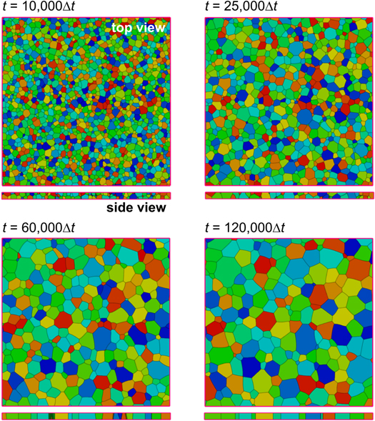
Figure 2. Microstructural evolution during grain growth simulation with film thickness h = 63Δx, starting from the initial structure shown in figure 1. Each panel shows the top and side views of part of the entire domain indicated by the red frame in figure 1.
Download figure:
Standard image High-resolution image3.1. Grain growth kinetics and morphology
This section investigates the kinetic and morphological characteristics of grain growth while focusing on their transitions from 3D to 2D growth modes. First, to quantitatively evaluate the 3D–2D transition of microstructures, we calculated the temporal variations in the number fraction of 2D-like columnar grains, fcolum, for each film thickness h. Here, grains that appear both on the top and bottom surfaces of the domain are defined as columnar ones. The results are shown in figure 3, from which we can see that all of the curves appear to be sigmoidal shaped. However, with increasing h, the rate of increase in fcolum significantly decreases. If we compare the results for h = 47Δx and h = 95Δx, the time required for the development of a fully columnar structure (i.e. fcolum ≈ 1) is almost four times larger in the latter case than in the former case.

Figure 3. Temporal variations in the number fraction of columnar grains fcolum, as calculated for films with different thickness h.
Download figure:
Standard image High-resolution imageNext, we examined grain growth kinetics. Figure 4 shows temporal variations in squared average grain size, 〈r〉2, for different film thickness. Here, grain sizes on the top and bottom surfaces (rsur) and those in the middle section (rmid) of the domain are measured as their in-plane area (A)-equivalent radius (A/π)1/2. The dotted lines indicate the times at which the columnar grain fraction fcolum shown in figure 3 reaches 0.5 and 0.99. For comparison, we also plotted the results for the cross sections of a 3D bulk system and for a full 2D system, which were obtained from the previous large-scale MPF simulations of ideal grain growth [56]. For steady-state ideal grain growth, it is well known that the kinetics of the system follows the parabolic growth law [57–60]:

where t0 is the initial time and k is a constant. In all panels of figure 4, both 〈rmid〉2 and 〈rsur〉2 are observed to follow the parabolic law at relatively early and late stages of grain growth. However, for the early stages, while the temporal changes in 〈rmid〉2 coincide with that of the cross sections of a 3D bulk, the 〈rsur〉2 values increase visibly faster compared to them. Subsequently, the increases in 〈rmid〉2 are significantly accelerated around fcolum = 0.5, after which the grain growth rates in the surfaces and internal regions gradually decrease and converge to the identical one in the vicinity of fcolum = 1. Then, the slopes of size-time curves of thin-film grain growth approach that of the full 2D growth. The origin of the decrease in grain growth rates during the formation of columnar microstructures can be understood as follows: the zero-flux boundary condition used in the simulations guarantees that the grain boundaries migrate so as to form local contact angles of 90° with the surfaces. Therefore, once grain boundaries reach both the top and bottom surfaces, their through-thickness curvatures gradually decrease to zero due to interfacial tension. Finally, 3D grains become equivalent to 2D polygonal ones. Because the driving force (interfacial curvature) for 2D grain growth is generally smaller than that for 3D growth [56, 58], such change in the geometrical characteristics of grains results in the decrease in the slopes of grain size-time curves.
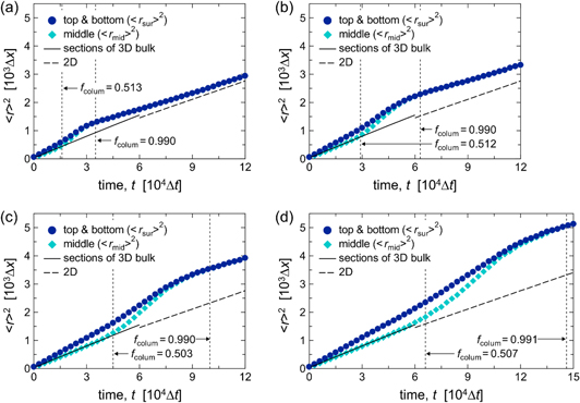
Figure 4. Temporal variations in squared average grain size on the top and bottom surfaces and middle section of the film, as calculated for different film thickness: (a) h = 47Δx, (b) h = 63Δx, (c) h = 79Δx, and (d) h = 95Δx. The solid lines show the previous MPF simulation result [56] for the cross sections of a 3D bulk system at t ≤ 60 000Δt, whereas the dashed lines show that for a full 2D system at t ≥ 60 000Δt.
Download figure:
Standard image High-resolution imageThe above results confirm that the 3D–2D transition of growth kinetics takes places around fcolum = 0.5 and gets accomplished near fcolum = 1 for all conditions of film thickness. We observed a similar transition behavior for the morphological characteristics of grain growth, namely, grain size distribution. As examples, figure 5 shows the temporal variations in normalized grain size distributions on the surfaces (rsur/〈rsur〉) and in the middle section (rmid/〈rmid〉), as calculated for film thickness of h = 47Δx and h = 79Δx. Here, the results are given for the times at which the columnar grain fraction fcolum is approximately 0.3, 0.5, 0.8, and 0.99. For comparison, the steady-state size distributions [56] for the cross section of a 3D bulk system and for a full 2D system are also depicted. As can be seen in the panels of figure 5, interestingly, grain size distributions on the surfaces exhibit a symmetrical shape similar to that of a full 2D system, even in the 3D growth regimes (fcolum ≈ 0.3, 0.5). On the other hand, at early stages (fcolum ≈ 0.3), size distributions in the middle section show common features with the bulk cross sections in terms of their right-skewed shapes and relatively long tails toward the large grain sizes. After fcolum ≈ 0.5, the distributions in the middle section gradually converge to those of the surfaces, and become almost identical around fcolum ≈ 1. It was confirmed from the results in figure 5 that, when the values of fcolum are almost the same, grain size distributions for films with different thickness take very similar shapes.

Figure 5. Temporal variations in grain size distribution on the top and bottom surfaces and middle section of the film, as calculated for film thickness of (a) h = 47Δx and (b) h = 79Δx. The solid and dashed lines show the steady-state size distributions from the previous MPF simulations [56] for the cross sections of a 3D bulk system and for a full 2D system, respectively.
Download figure:
Standard image High-resolution image3.2. Scaling of thin-film grain growth
The results presented in the previous section indicate that the thin-film grain growth behavior is uniquely determined by the columnar grain fraction fcolum, irrespective of film thickness. Herein, we discuss a way of comprehensively describing the grain growth in thin films with different thickness.
First, let us consider the theory of columnar structure formation reported by Walton et al [18]. According to their theory, if films have fully random initial structures with a similar average grain size, their columnar grain fraction fcolum during grain growth can be expressed by a function using only the ratio of time t to squared film thickness h2, namely, as fcolum = fcolum (t/h2). That is, if we use a scaled time τ = t/h2 instead of t, fcolum for films with different thickness is expected to take identical values at a given time τ. Note that, although the theory of Walton et al [18] is constructed using a 2D model of a through-thickness plane of thin film (corresponding to the side views in figure 2), the outline of the derivation may also hold for 3D by replacing 'length' with 'area' in their arguments. To test the above scaling law, we calculated and plotted the temporal variations of fcolum for different film thickness as a function of τ = t/h2, as shown in figure 6. In the figure, the fcolum versus τ curves for different thickness are almost perfectly overlapped. It is evident, therefore, that fcolum of 3D films follows the scaling law of Walton et al.

Figure 6. Number fractions of columnar grains fcolum as a function of scaled time τ = t/h2, as calculated for films with different thickness h.
Download figure:
Standard image High-resolution imageNext, we focus on the scaling of grain growth kinetics. Provided the mode of grain growth is dependent solely on the fcolum value, growth kinetics (variation in grain size) is expected to also follow some scaling rule, as with the case of fcolum; here, we test this idea. Dividing both sides of the parabolic law (equation (3)) by h2 roughly estimates that, if time t is scaled by τ = t/h2, squared average grain size 〈r〉2 also scales as 1/h2:

the validity of this prediction can be observed in figures 7(a) and (b), where the increases in the square of the scaled average grain sizes, 〈r〉2/h2, are given as functions of τ, respectively for the surfaces and middle section of the films with different thickness. As can be seen in these figures, the scaled grain sizes exhibit a very good agreement with each other, similarly to the case of fcolum.

Figure 7. Increases in the square of scaled average grain size 〈r〉2/h2 as a function of scaled time τ = t/h2, as calculated for the (a) top and bottom surfaces and (b) middle sections of films with different thickness h.
Download figure:
Standard image High-resolution image
The results summarized above enable us to conclude that grain growth behaviors in thin films with random initial structures are identical under uniform magnification of 1/h2 and, thus, can be comprehensively described irrespective of film thickness.
4. Conclusions
In this study, we investigated grain growth in polycrystalline thin films via 3D simulations. Ideal free surfaces were modeled by zero-flux boundaries. Utilizing the MPF model and parallel GPU computation, a series of large-scale simulations with approximately one million initial grains were performed for systems with different thickness. This enabled detailed analysis on the correlations between the film thickness and statistical characteristics of grain growth. The main findings are summarized as follows:
- (1)At relatively early stages, grain growth behaviors in the surfaces and middle section of a film are clearly different in terms of the average and distribution of grain sizes; while the latter is consistent with that of the cross sections of a 3D bulk, the former does not match it. After that, they gradually converge to full 2D growth with the development of a columnar grain structure.
- (2)When grain growth in films with different thickness is directly compared, their 3D–2D transition behaviors and resultant growth kinetics apparently differ with each other. However, by applying the scaling with 1/h2, they can be described in a unified manner, independent of the thickness.
This study examined the fundamental points of grain growth in thin samples by focusing on an ideal system, which is free from thermal grooving, precipitates, non-equiaxed initial grain shapes, and anisotropy in grain boundary and surface properties. However, these factors may significantly affect the nature of thin-film grain growth. For instance, grain growth in real thin films often encounters stagnation and subsequent abnormal growth, which were not observed in the present simulations. Therefore, our future work will study thin-film grain growth in more realistic systems. For such attempts, the ideal system investigated here will be useful as a yardstick for quantifying the effects of the complicated factors.
Acknowledgments
This research was supported by Grant-in-Aids for Scientific Research (B) (No. 16H04490) and for JSPS Fellows (No. 17J06356) from the Japan Society for the Promotion of Science (JSPS), and a Grant-in-Aid for Scientific Research (S) (No. 26220002) from the Ministry of Education, Culture, Sports and Technology (MEXT), the Joint Usage/Research Center for Interdisciplinary Large-scale Information Infrastructures, and the High Performance Computing Infrastructure in Japan. This work was also partially supported by 'Joint Usage/Research Center for Interdisciplinary Large-scale Information Infrastructures' and 'High Performance Computing Infrastructure' in Japan (Project ID: jh180036-NAH).