

Abstract
We propose a Lagrangian method for simultaneous, volumetric temperature and velocity measurements. As tracer particles for both quantities, we employ encapsulated thermochromic liquid crystals (TLCs). We discuss the challenges arising from color imaging of small particles and present measurements in an equilateral hexagonal-shaped convection cell of height h = 60 mm and distance between the parallel side walls w = 104 mm, which corresponds to an aspect ratio  . As fluid, we use a water-glycerol mixture to match the density of the TLC particles. We propose a densely-connected neural network, trained on calibration data, to predict the temperature for individual particles based on their particle image and position in the color camera images, which achieves uncertainties below 0.2 K over a temperature range of 3 K. We use Shake-the-Box to determine the 3D position and velocity of the particles and couple it with our temperature measurement approach. We validate our approach by adjusting a stable temperature stratification and comparing our measured temperatures with the theoretical results. Finally, we apply our approach to thermal convection at Rayleigh number Ra =
  and Prandtl number Pr = 10.6. We can visualize detaching plumes in individual temperature and convective heat transfer snapshots. Furthermore, we demonstrate that our approach allows us to compute statistics of the convective heat transfer and briefly validate our results against the literature.
Export citation and abstract BibTeX RIS

Original content from this work may be used under the terms of the Creative Commons Attribution 4.0 license. Any further distribution of this work must maintain attribution to the author(s) and the title of the work, journal citation and DOI.
1. Introduction
Temperature-driven flows are ubiquitous. They are responsible for many earthbound [1–5] and astrophysical phenomena [6, 7] and thereby have a direct impact on our daily life. Beyond the occurrence in nature, convective heat transfer is important in many engineering applications on different scales [8], e.g. the cooling of electronic components [9] or inherent temperature-driven flows in large scale energy storages [10], to name just two. Hence, a deep understanding of the underlying mechanism and the convective heat transfer, in general, is essential.
In many cases, however, the specific configurations are too complex and can not be efficiently modeled. Therefore, the simpler, canonical Rayleigh–Bénard convection (RBC) model is often studied instead. In the idealized RBC model, a fluid is confined by adiabatic sidewalls, heated from below, and cooled from above. Once a critical temperature difference between the cooling and heating plate is reached, fluid motion sets in due to local fluid density changes. The emerging convective flow is governed by two dimensionless numbers, namely the Rayleigh number Ra  , which is a measure of the ratio between the strength of the thermal driving and viscous damping, and the Prandtl number Pr
  as the ratio of the momentum to thermal diffusion, respectively. In these definitions, g denotes the acceleration due to gravity, α the thermal expansion coefficient,
  the temperature difference between the cooling and the heating plate and h the height of the domain. ν and κ represent the kinematic viscosity and the thermal diffusivity, respectively. Beyond Ra and Pr, the aspect ratio
  and shape of the container affect the flow and the formation of characteristic structures [11, 12]. Since the first systematic studies [13, 14] thermal convection has been extensively studied by means of experimental, numerical and theoretical methods [15, 16]. Nevertheless, the flow phenomena are not yet fully understood, and many open questions, for example, with respect to the thermal boundary conditions [17, 18] remain.
Even though the power of high-performance computers is ever-increasing, not all problems are viable to be solved by numerical studies. Hence, experiments are still essential, especially when studying flow configuration apart from the classical idealized setup.
While volumetric velocity measurements in fluids are now state-of-the-art [19–22], volumetric temperature measurements, especially combined with velocity measurements, remain the exception.
Massing et al [23] and Deng et al [24] combined luminescent lifetime imaging, which leverages the temperature-dependent intensity decay rate of exited photoluminescent particles and astigmatism particle tracking velocimetry (APTV) for a joint study of temperature and velocity on the micro-scale. This technique, however, is not well suited for long-time measurements due to the photobleaching effect. Also, on a micro-scale, Segura et al [25] combined particle image thermometry (PIT) with non-encapsulated thermochromic liquid crystals (TLCs) and APTV to measure temperature and velocity within an evaporating droplet. All these approaches are well-suited for microfluidic measurements since they use only a single camera. However, APTV measurements require large particle images, limiting the field of view and spatial resolution of the measurement and therefore are less suitable for macroscopic flow measurements [26].
Stelter et al [27] developed a thermographic 3D Particle Tracking Velocime (PTV) approach. They use the temperature-related spectral shift of the emission spectrum of phosphorous particles, which were excited by an ultra-violett laser. They were able to measure the temperature within a hot jet but were limited to low seeding concentrations. Kashjan and Nobes [28] applied a scanning approach to 2D two-color laser-induced fluorescence. By scanning several parallel planes in rapid succession, they could reconstruct the temperature distribution within a slender RBC cell. This approach can, in principle, also be combined with particle image velocimetry (PIV) measurements. Kimura et al [29] combined a scanning planar PIV and PIT approach to reconstruct 3D temperature and velocity distributions in rotating thermal convection. The applicability of their technique is limited due to the requirement of a rotating experiment. Furthermore, a rotating domain influences the flow physics [30]. Rietz et al [31] investigated the usage of TLCs and a light field camera for joint 3D temperature and velocity estimation on a qualitative level. Closest to the method presented in this work is the study by Schiepel et al [32]. In their work, they combined tomographic PIV and PIT to investigate RBC. Even though they successfully reconstructed both temperature and velocity, the authors combined an Eulerian approach for the velocity measurement and a Lagrangian approach for the temperature measurements, leading to significant processing overhead due to the tomographic processing itself as well as the necessity to identify the individual particles within the reconstructed intensity volume.
In this manuscript, we describe a purely Lagrangian approach for simultaneous temperature and velocity measurements in a volume. Namely, we combine Lagrangian Particle Tracking with TLC-based PIT [33, 34] and apply it to an RBC experiment. The Lagrangian approach yields efficient processing and allows us to study the heat transfer along the particle trajectory. We leverage the temperature-related color change of the light scattered by the TLC particles for temperature estimation. We implement a deep learning approach to estimate the temperature from individual particle images and the particle image positions in the color camera image, similar to the method presented by Noto et al [35] for color-based depth regression in color PTV. This approach benefits from the additional information provided by the whole particle images compared to a single averaged color value. Therefore, it is robust to local, non-temperature-related changes in the TLCs' color appearance.
The remainder of the manuscript is structured as follows. In section 2, we discuss the challenges that arise from color imaging of small particles. Thereupon, section 3 introduces the experimental setup, followed by a detailed explanation of the developed method in section 4. Subsequently, we validate our results and apply the method to RBC in section 5. Finally, we summarize our manuscript and provide an outlook in section 6.
2. Color imaging of small particles
For the vast majority of particle-based optical flow measurements, only the fluid velocity is measured, and hence, monochromatic cameras are used [36]. In our case, however, color imaging is essential to analyze the TLCs' color, which contains information about their temperature. Here two distinct challenges arise, which are specifically important when small particles are imaged, namely the color separation of the camera and chromatic dispersion.
2.1. Color separation
The camera pixels are the light-sensitive elements on the camera sensor. In general, a pixel does record light intensities and does not differentiate between the wavelength of the incident light. Hence, the color must be separated before the pixel absorbs the light. Several different approaches have been developed. The by far most widespread method is to mount a fixed color filter array (CFA), e.g. a Bayer pattern as shown in figure 1(a), directly on top of the image sensors. Hence, only light passing the filter is absorbed by the respective pixel below. Due to the filter array, the image's actual resolution is reduced, and the RGB (red–green–blue) color image must be reconstructed or demosaiced from the raw image data. In the past, several demosaicing approaches have been proposed [37–39]. Many of these approaches take image features like edges or a larger region of the image into account to increase the reconstruction performance and minimize artifacts [40, 41]. While these advanced approaches work well for aesthetic photography, for the reliable temperature measurement from small particle images, these approaches can corrupt results by incorporating background regions into the reconstruction of the particle images' color.
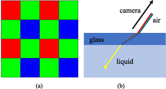
Figure 1. (a) Sketch of the color filter array called Bayer pattern. (b) Schematic of the chromatic dispersion at media interfaces.
Download figure:
Standard image High-resolution imageBeyond the CFA, there are other color separation approaches, like the so-called three-chip camera, which uses a trichroic prism for color separation, the Foveon X3 sensor, which separates colors by the wavelength-dependent penetration depth of the light, or the filter wheel camera. While the three-chip camera records full-resolution color images and hence no interpolation is required, the trichroic prism leads to a sharp color separation with minimal overlap between the color channels [42]. Hence, gradual changes in the particle image hue, as typical in PIT, might not be resolved by the three-chip camera. The Foveon X3 sensor, however, was, to the best of our knowledge, never used in a scientific camera and was discontinued. Finally, the filter wheel camera records the color subsequently and is therefore not well suited to image moving particles [43].
Considering all these aspects, a Bayer pattern camera combined with bilinear demosaicing turned out to be the most suitable choice and is also available in many other laboratories; however, a large enough particle image size is essential.
2.2. Chromatic dispersion
When observing objects under polychromatic illumination through media with changing index of refraction and under oblique viewing angles, chromatic dispersion occurs as conceptualized in figure 1(b). While chromatic dispersion might be neglected when imaging large objects, it can seriously corrupt the color signal of small particle images. The effect might not always be severe but should nevertheless be considered when designing the experimental setup and applying the technique. Chromatic dispersion can be minimized by limiting the media interfaces in the optical path, matching the index of refraction, the usage of lenses with large focal lengths and suitable camera positioning.
3. Experiment
The experiments were performed in an equilateral hexagon-shaped convection cell made from glass with a height h = 60 mm and a distance between parallel sides w = 104 mm, corresponding to an aspect ratio  . The hexagonal shape was chosen to allow for an oblique viewing angle into the illuminated volume and to keep the camera viewing direction perpendicular to the sidewall. Thereby, chromatic dispersion as described in section 2 can be minimized. An image of the experiment is shown in figure 2. Both the cooling and heating plates are made from aluminum, which was chosen due to its high thermal conductivity. The temperature in both plates can be adjusted by pumping water through a meander structure inside the plate.

Figure 2. Image of the experimental setup. The thermostats and the connecting hoses are not shown.
Download figure:
Standard image High-resolution imageThe temperature in each plate is measured by a PT-100 thermistors with a maximum deviation of 0.1 K at 0 ∘C. However, the deviation of the individual temperature sensors to each other was found to be below 0.01 K. During the experiment, a volume of ≈12 mm in the depth direction z at the center of the cell was illuminated by a custom-made light source with a spectrum covering the visible range. The light source is a smaller version of the LED light source used by Moller et al [44]. It was used in pulsed mode with a pulse width of 20 ms to avoid motion blur and illuminated the full cell height. Since white light is necessary for the TLCs, LEDs are a good choice due to their wide illumination spectrum and minimal energy input that may cause local heating.
The flow is captured by three cameras (PCO edge 5.5), of which one is color-sensitive. The camera arrangement is shown in the sketch in figure 3, which also includes the coordinate system's orientation. The cameras were positioned approximately 60 cm away from the center of the cell and observed the domain under an observation angle φ of 60∘ and 120∘, respectively. We used Scheimpflugadapters to optimize the depth of field. All cameras were equipped with achromatic, 100 mm focal length optics (Zeiss Milvus 2/100 M). We chose the observation angle  for the color camera since it is well suited for our experiment concerning the measurable temperature range and sensitivity while looking perpendicularly through the side walls. The two monochrome cameras were positioned to have a suitable stereo angle with the color camera while still looking through the sidewalls perpendicularly. Detailed information about optimizing the camera angle for the temperature and velocity measurements can be found in [34, 45]. We observed that due to the CFA, approximately 50% less light reached the sensor of the color camera compared to a monochrome camera in a similar configuration. The camera setup was geometrically calibrated using the 058-5 calibration target (LaVison GmbH) and a polynomial approach. Afterward, we refined the calibration by applying the volumetric self-calibration onto the particle images [46]. The geometric camera calibration was performed using DAVIS 10.2 (LaVison GmbH). As seeding particles encapsulated TLCs with a nominal diameter of 100 μm (Japan Capsular Products Inc.) were used. The particles have a nominal (
 ) temperature range from 20 ∘C where they start to appear red up to 30 ∘C when they appear blue and eventually become transparent again. However, in the current setup, the effective temperature range is drastically reduced to ≈ 19.7 ∘C – 22.7 ∘C due to the larger observation angle resulting in increased sensitivity. For further details on the influence of observation angle φ we refer the reader to [34]. For the experiment, the particle slurry was sieved, and only the fraction with a diameter between 63 μm and 100 μm was used as seeding particles. Since the density of the particles is slightly higher than water, a water-glycerol mixture with a volume fraction of 13% glycerol at room temperature was used to minimize sedimentation and floating of the particles.

Figure 3. Sketch of the top view inside the hexagonal cell. The drawing indicates the camera arrangement and the illuminated volume.
Download figure:
Standard image High-resolution image4. Processing
4.1. Temperature calibration
To derive the temperature from the particle images, a calibration that connects particle images and temperature has to be established. A flowchart of the procedure is shown in figure 4. We start the calibration by setting a uniform temperature distribution inside the convection cell by connecting the bottom and top plates both to the same thermostat. While adjusting the temperature, the fluid is stirred by a magnetic stirrer to enhance the heat transfer between plates and fluid. Thereby, a uniform temperature distribution can be achieved. After the temperature converged towards the set value, color images of the TLC seeding particles were recorded while the temperature was simultaneously measured by the PT-100 thermistors in the bottom and top plates to obtain the reference temperature  . Hence, the color appearance of the particles and the temperature can be connected. This procedure is performed in total 16 times from 19.7 ∘C to 22.7 ∘C with steps of 0.2 K to resolve the color response of the particles within this range.

Figure 4. Flowchart of the calibration procedure. An example input of the neural network is shown at the bottom right of the figure. MSE is the abbreviation for mean squared error, which is a common loss metric for training neural networks. It is defined in equation (1).
Download figure:
Standard image High-resolution imageSubsequently, we applied a simple bilinear interpolation to reconstruct the color information from the CFA image of the camera. Figure 5 shows excerpts of the color images at different reference temperatures. By comparing the temperature-related color difference of the particle images between the subfigures, the trend from red for low temperatures over green towards blue for high temperatures is recognizable. This is further verified by the circular mean hue value  written on top of each subfigure. The hue H is a measure that describes the perception of a color. It is a circular scale in which H = 0 is equal to H = 1. For more information on the hue values in the context of PIT, we would like to refer to the work by Moller et al [34]. Overall, the color difference between the particle images in the same subfigure is small but directly contributes to the measurement uncertainty. We then computed a grayscale version of the image and applied thresholds to negate background noise and over-saturated particles. We used
  and
and  as lower and upper thresholds, respectively. 65535 is the maximum intensity value in a 16-bit image. Subsequently, a local maxima search was performed to identify the particle images. We used the obtained position of the local maxima to extract the
  pixels particle color images. The extracted particle images were normalized by the maximum intensity across all pixels and color channels. Thereby we compensate for the intensity changes due to varying particle size and position within the illuminated domain. Thereupon, the particle image, as well as the position of the center pixel in the color image X and Y, totaling 77 input features, were split into training and testing sets with a ratio of 9:1. An exemplary input is shown at the bottom right of figure 4. Subsequently, the training data was forwarded into the machine learning pipeline for which we used the scikit-learn package [47]. This pipeline consists of the standard scalar preprocessing operation and an multi-layer perceptron regressor, which is a simple, densely-connected neural network, with three hidden layers of 100 neurons each and the Relu activation function. To train the network, the Adam optimizer was used [48]. The neural network was trained for 18 epochs until the mean squared error (MSE) sufficiently converged for 10 consecutive epochs. The MSE (equation 1) is a common loss metric for the training of neural networks.
In the definition of the MSE, n represents the number of samples or, in our case, particle images.
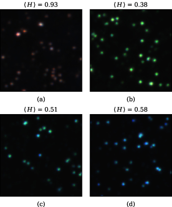
Figure 5. Exemplary images of TLC particles at 19.7 ∘C (a), 20.6 ∘C (b), 21.7 ∘C (c), and 22.7 ∘C (d). On top of each subfigure, the circular mean hue  is shown. It is a circular scale in which H = 0 is equal to H = 1 [34].
Download figure:
Standard image High-resolution imageIn the next step, we applied the neural network to the test data set to analyze the calibration quality and estimate the measurement uncertainty. In figure 6(a), we plotted the mean of the measured particle temperatures for each calibration step  depicted as blue stars over the reference temperature
  obtained from the PT-100 sensors for each calibration step. The dashed, gray line indicates
  , which denotes a perfect mean value of the predictions. One can clearly observe that the mean measured particle temperature
  and
and  agree well, except for the highest reference temperature, where the deviation is slightly higher since it is the upper limit of the training temperatures in the calibration data set.

Figure 6. (a) Plot of the mean measured particle temperature  (blue) for each reference temperature
  . The dashed, gray line indicates
  . (b) Plot of the mean absolute deviation between the reference and the measured particle temperature
  (red) and the standard deviation of the measured particle temperature σT
(blue) for each reference temperature
(red) and the standard deviation of the measured particle temperature σT
(blue) for each reference temperature  .
.
Download figure:
Standard image High-resolution imageFor a more detailed investigation of the model performance, we computed the mean absolute deviation between the reference temperature and the measured temperature  (red) as well as the standard deviation of the measured temperature σT
(blue) for each reference temperature, which is shown in figure 6(b). Looking at the mean absolute deviation, we observe it to be lower than the standard deviation except for the highest reference temperature. This indicates a small systematic deviation from the reference temperature. Furthermore, the standard deviation as a measure of the measurement uncertainty for all temperature steps is below 0.2 K, indicating a relative measurement uncertainty of
(red) as well as the standard deviation of the measured temperature σT
(blue) for each reference temperature, which is shown in figure 6(b). Looking at the mean absolute deviation, we observe it to be lower than the standard deviation except for the highest reference temperature. This indicates a small systematic deviation from the reference temperature. Furthermore, the standard deviation as a measure of the measurement uncertainty for all temperature steps is below 0.2 K, indicating a relative measurement uncertainty of  over the considered temperature range of 3 K.
4.2. Joint temperature and velocity measurements
After successful training, the neural network can be applied together with Shake-the-Box (STB) for joint temperature and velocity measurements as visualized in figure 7. We started by setting up the experiment and recording images with three cameras. After demosaicing the CFA images, we generated a gray-scale version of the color images. To demonstrate that the particle images of the color camera can be used for tracking, we compare a CFA particle image (a), a gray-scale converted particle color image (b), and a particle image recorded by a monochrome camera (c) figure 8. While the imprint of the CFA can be noticed in the CFA image, the intensity distribution of the gray-scale converted particle color image appears Gaussian, albeit larger than the particle image recorded by the monochrome camera. This proves that the demosaicing acts similarly to a smoothing filter and that the gray-scale converted particle color image is suitable for particle tracking even though the subpixel accuracy of the position estimation might be slightly lower than for the monochrome particle image. The exact influence of the demosaicing on the uncertainty of the position estimation should be investigated in future studies. Hence, the gray-scale converted color image, together with the images of monochrome cameras, were then processed using the time-series STB (Davis 10.2) [20]. Here, we used only a single processing path. After the STB processing, the 3D particle positions were back-projected into the image of the color camera and the particle images were extracted. The extracted particle images were thresholded by their mean intensity to discard over- and under-saturated particles or particles not present in the color camera image. However, due to the camera position with the two monochrome cameras opposing each other and, thereby, generating little additional perspective information, almost all the 3D position estimations require the particle image from the color camera. Hence, in theory, the temperature can be estimated for almost all tracked particles. We then took the particle image and the image coordinates as input for the trained neural network to estimate the temperature. Subsequently, the particle temperature data and the particle velocity data were merged. For the convection measurement, the particle temperatures were filtered using a sliding median filter with a window of three time steps on the respective trajectory, and trajectories shorter than five consecutive time steps were discarded.
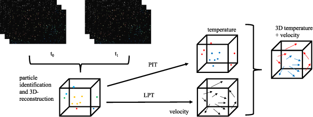
Figure 7. Conceptual sketch of the joint temperature and velocity measurements.
Download figure:
Standard image High-resolution image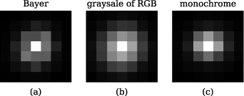
Figure 8. Comparison of a typical Bayer particle image (a), a gray-scale converted particle color image (b), and a particle image recorded by a monochrome camera (c).
Download figure:
Standard image High-resolution image5. Results
To validate our method, we set a stable thermal stratification in the flow domain by cooling the bottom plate to 19.9 ∘C and heating the top plate to 22.4 ∘C. Hence, heat is only conducted, and in an idealized setup, a well-known linear temperature profile would emerge. Figure 9(a) shows a scatter plot of the temperature of the particles in the  plane. The plots contain data from 200 snapshots. Looking at the scatter plot, we can clearly identify the trend from low temperatures at the bottom up to high temperatures at the top, with only a few apparent outliers. For better quantification, we partitioned the cell height into 19 equally spaced horizontal bins and computed the average temperature and the standard deviation for each bin. Figure 9(b) shows the resulting vertical temperature profile
  . Each blue marker indicates the average temperature of its corresponding bin, and the bar shows the standard deviation of the temperature within the bin. The dashed line indicates the theoretical temperature profile that would emerge under the conditions of adiabatic sidewalls and pure conductive heat transfer between the plates. Comparing the measured vertical temperature profile with the theoretical profile shows that the measurements capture the trend. However, the profiles differ, especially at the mid-height of the cell. This deviation is caused by the boundary conditions of the sidewall, which do not adhere to adiabatic assumption, especially in the case of the linear temperature profile. The sidewalls are made from 6 mm thick glass with a thermal conductivity
  W mK−1, which cannot be further covered by insulation due to the necessity of optical access. Comparing the thermal conductivity with the thermal conductivity of the water-glycerol mixture
  W mK−1, we can see that the sidewalls do not achieve the thermal insulation required to be considered adiabatic, especially when the heat transfer in the fluid is not enhanced by thermal convection. Looking at the error bars, we see that the standard deviation within the bins increases with a temperature increase. This is related to the decreasing temperature sensitivity of the TLCs at higher temperatures.
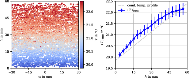
Figure 9. (a) Scatter plot of the temperature of individual particles T of the stable thermal stratification achieved by cooling the bottom plate and heating the top plate. The particle positions are projected in the x − y-plane. (b) Vertical temperature profile  obtained by binning the scatter plot data and averaging along the width. The bar indicates the standard deviation of the measured temperature within the corresponding bin.
Download figure:
Standard image High-resolution imageFinally, we applied the approach to the classical RBC setup. Therefore, we set the cooling plate temperature to  C and the heating plate temperature to
  C. Combined with the fluid properties, this results in a Rayleigh number Ra =
  and a Prandtl number Pr = 10.6. At this point, we want to emphasize that the temperature difference between the plates is larger than the sensitivity range of the TLCs. Hence, the thermal boundary layer can not be resolved by the TLCs; in return, however, the bulk fluctuations of the temperature can be well resolved. After an initial waiting phase in which the flow established, a time series of 1000 images was recorded at a frame rate of 10 frames per second, resulting in a measurement time t = 100 s. This time span corresponds to a dimensionless time of 71 free-fall units with a free fall time
  = 1.40 s. After tracking and post-processing, we obtained the temperature and velocity of approximately 5000 particles per time step. For a better physical interpretation of the results, we non-dimensionalize the time, length, temperature, and velocity according to the equations (2)–(5), respectively,
Figure 10 shows an exemplary snapshot of the dimensionless temperature fluctuations

With  denoting the spatial and temporal average the dimensionless temperature
  . Looking at the figure, we can clearly see the detaching thermal plumes and the fluctuations within the bulk. Remarkably is also the hot region close to the cooling plate at
  , hinting at the presence of the large-scale circulation (LSC) typical for convection cells with an aspect ratio close to unity [49, 50]. Comparing the structures in the temperature snapshot with those in the snapshot of the velocity magnitude, shown in figure 11, we observe that particles with a larger difference from the mean temperature have a large velocity magnitude. This is intuitive since the local fluctuations in the density, caused by local temperature fluctuations, drive the fluid motion. We distinguish higher velocity magnitudes close to the heating and cooling plate and the vertical edges of the shown region compared to the center, again indicating the presence of the LSC. The LSC organizes along the domain diagonal and is therefore tilted around the vertical axis with respect to the volume of interest.
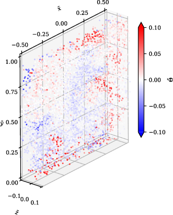
Figure 10. Exemplary temperature fluctuation  snapshot of RBC. A video of the whole time series can be found in the online supplementary materials.
Download figure:
Standard image High-resolution image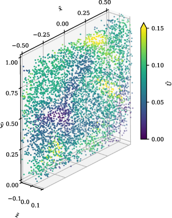
Figure 11. Exemplary velocity magnitude  snapshot of RBC. A video of the whole time series can be found in the online supplementary materials.
Download figure:
Standard image High-resolution imageThe significant advantage of our purely Lagrangian approach is that we are able to study the convective heat transfer in time and space along particle trajectories. As these are highly aligned to the thermal plumes this allows for a complete characterization of the structures in space and time. Hence we compute the convective heat transfer according to (7), similar to [51, 52],

The definition of the convective heat transfer is equal to the definition of the local Nusselt number [17, 53]. However, since the local Nusselt number represents the overall heat transfer, the conductive heat transfer must be neglectable, which is only a valid assumption close to the horizontal mid-plane within the Boussinesq-approximation regime. Hence, in our case, the convective heat transfer should not be interpreted as the local Nusselt number. Figure 12 shows the convective heat transfer  for the same snapshot as shown in figures 10 and 11. The plot unveils the enhanced heat transfer of the thermal plumes compared to the heat transport of the turbulent background. We also observe regions of inverted convective heat transfer (blue) close to the thermal plumes. Animations of the temperature fluctuations
  , the velocity magnitude
  , and the convective heat transfer
  are available as online supplementary material. Apart from analyzing single snapshots or animations, the simultaneous temperature and velocity data can be used to compute the heat transfer statistics. To demonstrate that, we calculate the probability functions (PDF) of the normalized convective heat transfer
  with
with  indicating the standard deviation of
  . The probability density function shows the relative likelihood of a fluid parcel being associated with a convective heat transport within a specific range of values.
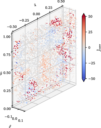
Figure 12. Exemplary convective heat transfer  snapshot of RBC. A video of the whole time series can be found in the online supplementary materials.
Download figure:
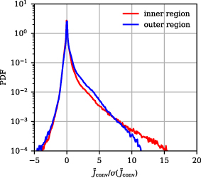
Standard image High-resolution imageIn figure 13 the PDFs of  for the inner region
  (red) and outer region
  (blue) are shown. Both PDFs show the typical skew towards positive events, which are more likely since, in RBC, heat is transferred from the bottom to the top. We compare the results with the PDFs presented by Shang et al [52], obtained from point-wise measurements at the center of the cell and near the sidewall. Albeit their measurements were performed at Ra
  and Pr ≈ 5.5, we observe that the shape, especially of the PDF of the inner region, is similar to the respective counterpart shown by Shang et al. The PDF of the outer region and the sidewall PDF by Shang et al are less similar since even the outer region can not be considered as close to the wall. Nevertheless, the same trend towards less extreme
  events at the sidewall is also apparent in the PDF of the outer region. This shows that the joint measurement technique can be used to measure the statistics of the heat transfer and once more underlines the capabilities of the proposed method.
Figure 13. PDF of the normalized convective heat transfer  for the inner region
  (red) and outer region
  (blue).
Download figure:
Standard image High-resolution image
6. Conclusion
In this paper, we presented a purely Lagrangian approach for simultaneous and volumetric temperature and velocity measurements in liquids. We employ temperature-sensitive encapsulated TLCs as seeding particles for the temperature as well as the velocity measurements. We discuss the challenges that arise from color imaging of small particles and propose possible solutions. The particle velocities and 3D positions are obtained from the commercial version of the STB algorithm. We propose a novel temperature processing method based on a neural network that uses the whole particle images as well as their position within the camera image and hence can compensate for local changes in the particle images as they would occur due to chromatic dispersion and varying viewing angles for large fields of views. We evaluate our approach on the test dataset and obtain relative uncertainties of  . We furthermore validate our method on a stable thermal stratification by heating the top plate and cooling the bottom plate. We correctly catch the gradual change of the temperature over the cell height; however, some deviations in the bulk are observed. This is caused by the non-adiabatic sidewall, which due to the low thermal conductivity of the fluid compared to the wall material, can not be considered as a thermal insulator, especially for the case of purely conductive heat transfer within the fluid. Finally, we apply our technique to RBC at Ra =
  and Pr = 10.6. We are able to clearly visualize detaching thermal plumes as well as the LSC. Our joint method allows us to determine the convective heat transfer of individual particles and, hence, to study the statistics of the convective heat transfer. In the future, we will focus on further developing the temperature measurement technique by improving the processing and post-processing to detect and replace outliers more effectively to allow for higher seeding densities. However, color ambiguities due to overlapping particles are limiting the seeding density. To circumvent this and to reduce the uncertainty of the temperature measurement, we are currently working on integrating another color camera into the setup. Judging from the particle images in figure 8, we believe that the uncertainty of velocity measurement will remain low, but this should also be addressed in a dedicated study. Beyond that, we aim for a deeper integration of the temperature measurements within the 3D particle tracking algorithm to reduce the computational cost. Another aspect is the development of a joint data assimilation technique to extract Eulerian fields that take advantage of the available temperature data. Finally, we want to apply the new method to study large aspect ratio RBC [17] and thermal energy storages [54].
Acknowledgments
We gratefully acknowledge the help of Tobias Röckl with the experiments and Thomas Rockstroh for the support with the back-projection of the particles. We also want to thank Thomas Fuchs for the fruitful discussions. This work was supported by the Carl Zeiss Foundation within Project No. P2018-02-001 'Deep Turb—Deep Learning in and of Turbulence'. and by the DFG Priority Program SPP 1881 on 'Turbulent Superstructures' within Project No. 429328691.
Data availability statement
The data cannot be made publicly available upon publication because they are not available in a format that is sufficiently accessible or reusable by other researchers. The data that support the findings of this study are available upon reasonable request from the authors.
Conflict of interest
There are no conflicts of interest to declare.
Convective heat transfer (10.2 MB MP4) Video of the time series that shows the convective heat transfer.
Temperature fluctuation (9.9 MB MP4) Video of the time series that shows the temperature fluctuation.
Velocity magnitude (19.8 MB MP4) Video of the time series that shows the velocity magnitude.