


Abstract
The frequency-shift demodulation is a primary demodulation method in phase-sensitive optical time domain reflectometry (Φ-OTDR) with intrinsic resistance to interference fading. So far, the least mean squares (LMS) estimation method has the optimal demodulation accuracy and robustness. However, it takes much processing time due to the step-by-step sliding operation. In this work, we propose a fast LMS estimation method based on cross-correlation calculation to accelerate the demodulation while maintaining accuracy. Experiments are performed along a 9 km sensing fiber with a 4 m spatial resolution. The performance of the fast LMS, LMS, and cross-correlation methods are compared by using the same parameters. Compared with the LMS method, the fast LMS achieves a 12-time improvement in processing speed while remaining the same demodulation accuracy. Although the proposed fast LMS method takes slightly more time than the cross-correlation method (1.6 times), it improves the demodulation accuracy ∼6 dB for the vibration signal and ∼2.1 dB for the overall demodulation accuracy.
Export citation and abstract BibTeX RIS
1. Introduction
Over the past few decades, distributed optical fiber sensors have evolved rapidly [1–3]. Among the numerous distributed fiber sensors, phase-sensitive optical time-domain reflectometry (Φ-OTDR) has attracted a lot of attention due to its advantages of fast response speed and high sensitivity [1,4,5]. Till now, Φ-OTDR has been demonstrated for dynamic and static sensing detection scenarios, including pipeline detection, structural health detection, acoustic detection, etc [6–8].
Generally, a high-coherence laser source is required to generate the probe pulse in Φ-OTDR. The probe pulse travels through the fiber, producing Rayleigh backscattering (RBS) at different scattering points. The generated RBS lightwaves interfere with each other, resulting in fluctuating light intensities. When vibration or temperature is applied to the fiber, the fiber distance between different scatters is changed, thereby resulting in changes in optical intensity and phase. In the beginning, the external perturbances are detected by analyzing intensity changes in Φ-OTDR [9–12]. With this method, the perturbance location can be accurately determined but the time and frequency properties of the perturbance cannot be retrieved. Different from the intensity of the RBS signal, the phase difference between two different RBS signals is linearly proportional to the applied strain in the fiber segment between these positions [13, 14]. Based on this theory, phase-demodulation schemes are proposed to recover dynamic strains [13–18]. However, the selection of RBS signals must be outside both ends of the vibration section, resulting in a reduced spatial resolution. Additionally, phase demodulation is susceptible to interference fading, which significantly impacts the reliability and stability of this method [19, 20].
In addition to the above two demodulation methods, frequency-shift demodulation using a frequency-sweeping source can also be utilized for dynamic sensing in Φ-OTDR [21–24]. Unlike phase demodulation, this approach requires only one RBS signal within the perturbation zone to recover the dynamic strain, thus having a higher spatial resolution. Furthermore, this method is intrinsically immune to interference fading. In frequency-shift demodulation, a frequency-tunned pulse probe is first used and this method is time-consuming [21–24]. To improve the response speed, the frequency-swept process is replaced by a chirp pulse [25–27]. Recently, a pulse conversion algorithm is proposed to acquire an equivalent chirp detection signal, which avoids the complicated and expensive chirp modulation and is cost-effective [28]. In Φ-OTDR based on frequency-shift demodulation, the cross-correlation calculation is first used to estimate the frequency shift (FS) of signal spectra. However, the cross-correlation method is susceptible to noise and may introduce an estimation error (ER). To improve the robustness of demodulation, the least mean squares (LMS) algorithm is proposed and it avoids large random errors [23, 29]. Nevertheless, the LMS algorithm dramatically increases the demodulation time due to the step-to-step calculation.
In this work, a fast LMS algorithm is proposed by expanding the expression of the LMS algorithm. According to the mathematical relations, the time-consuming operation of step-by-step sliding in the LMS algorithm can be replaced by the cross-correlation calculation, which greatly improves the processing speed. Experiments are implemented in a 9 km long sensing fiber with a probe pulse of 20 ns. Performance comparisons including computation time and demodulation accuracy are performed using fast LMS, LMS, and cross-correlation methods under the same conditions. The results show that the fast LMS method is consistent with the demodulation accuracy of LMS, and the demodulation speed is significantly improved. The proposed method is simpler and faster, which provides a new approach for fast and accurate demodulation of Φ-OTDR based on FS.
2. Operation principle
2.1. Spectra acquisition
In heterodyne coherent Φ-OTDR, a single-sideband signal I(t) is acquired. With Hilbert transform, the coressponding complex signal Ic (t) can be obtained with the following expression.

where H[ ] denotes Hilber transform. The complex signal Ic
(t) contains the sensing information of the entire fiber.
] denotes Hilber transform. The complex signal Ic
(t) contains the sensing information of the entire fiber.
In signal demodulation, a part of signal is extracted from Ic (t) with a window function and expressed as Iz (t).
where rect() denotes the rectangle function, tW denotes the time width of the rectangle function. tW determines the duration of the selected signal and the effective spatial resolution. tz
denotes the transmission time of the pulse from the fiber initial position to the fiber position z.
Subsequently, the extracted signal Iz (t) is convoluted with a chirp factor c(t) to acquire the equivalent signal sz (t) [28]. sz (t) is expressed as

where  denotes the convolution operator, sz
(f) is the complex frequency spectrum of Iz
(t), c(t) is described as
denotes the convolution operator, sz
(f) is the complex frequency spectrum of Iz
(t), c(t) is described as
In equation (4), PW, f0, and k are the chirped pulse width, initial frequency, and chirp rate of the chirp factor, respectively. k= B/PW, B is the bandwidth of c(t). Note that B used in signal demodulation is determined by the bandwidth of the probe pulse in Φ-OTDR system. With this operation, the FS (which corresponds to the applied strain) is converted into time shift with the following mathematical relationship [28].
where Δt denotes the time shift, fc is the center frequency of the probe pulse, Δf denotes the FS, Δ is the change of strain at position z. When
  , the amplitude of sz
(t) is close to the amplitude of sz
(f). Meanwhile, the time variable in sz
(t) can be converted into a frequency variable as follows.
, the amplitude of sz
(t) is close to the amplitude of sz
(f). Meanwhile, the time variable in sz
(t) can be converted into a frequency variable as follows.

where || denotes the modulo operator. Subsequently, the FS between two measured signals at the same position z (acquiring with two different probe pulses) is calculated using cross-correlation, LMS, and fast LMS algorithms.
2.2. Principle of the demodulation methods
In previous works, the FS between two signals is calculated using cross-correlation or LMS algorithms. The principle of the cross-correlation method is expressed as

where  denotes the cross-correlation result, Sz,i
(f) and Sz,j
(f) denote the amplitude spectra obtained from the ith and jth measurements at position z, respectively.
denotes the cross-correlation result, Sz,i
(f) and Sz,j
(f) denote the amplitude spectra obtained from the ith and jth measurements at position z, respectively. ![$i,j \in [1,N]$](https://content.cld.iop.org/journals/0957-0233/35/2/025101/revision2/mstad0687ieqn4.gif) and N represents the number of the collected RBS signals/traces. f1
and f2
are the initial and cut-off frequencies in the calculation.
and N represents the number of the collected RBS signals/traces. f1
and f2
are the initial and cut-off frequencies in the calculation.  denotes the relative FS. The FS
  is estimated by searching the index corresponding to the peak value. fM
determines the measurable range and is limited by the bandwidth of the probe pulse.
is estimated by searching the index corresponding to the peak value. fM
determines the measurable range and is limited by the bandwidth of the probe pulse.
Although the cross-correlation method is simple, it may introduce large demodulation errors and has bad robustness [23, 29]. To improve the robustness of the frequency-shift demodulation, the LMS algorithm is proposed [23, 29] and its operation principle is expressed as

In equation (8a
),  represents the result of LMS calculation. Notice that the spectrum used in LMS is same as that used in the cross-correlation calculation. Unlike searching the maximum value in the cross-correlation calculation, LMS algorithm searches the minimum value expressed as equation (8b
).
represents the result of LMS calculation. Notice that the spectrum used in LMS is same as that used in the cross-correlation calculation. Unlike searching the maximum value in the cross-correlation calculation, LMS algorithm searches the minimum value expressed as equation (8b
).
The LMS method achieves higher robustness and demodulation accuracy, but it takes much more time since the conventional LMS algorithm is implemented in a step-by-step calculation [23, 29]. Actually, the time-consuming calculation in the LMS can be replaced by some fast operations. Equation (8a ) can be expanded and rewritten as

In equation (9), the LMS method is decomposed into three parts including two sum-of-squares operations and one cross-correlation operation. The three terms  ,
,  , and
, and  are expressed as
With this replacement, the processing speed will be improved, especially for computing the large bandwidth signal. Similar to the LMS method, the output  in equation (9) is used to compute the relative FS with equation (8b
).
in equation (9) is used to compute the relative FS with equation (8b
).
The above explains the demodulation process of the relative FS using two traces at the same location. To obtain the complete sensing signal (FSs) for one position z, some additional operations are required. Generally, two methods are alternative:
- (1)setting i= 1 and increasing j from 2 to N, the demodulated result is the target sensing signal.
- (2)i is a variable that is increased from 1 to N−1 while j is equal to i ± 1. With this method, the demodulated results are the relative FSs between two adjacent traces, and all relative FSs must be integrated to obtain the target sensing signal.
In this work, the second method is adopted to obtain the target sensing signal at a certain location. To retrieve all sensing signals/FSs over the whole fiber, it is necessary to extract the RBS signals at different locations by varying variable tz in the window function (shown in equation (2)) and performing the above demodulation process.
3. Experimental setup and results
The experimental setup is depicted in figure 1, a narrow linewidth laser (NLL) with a center wavelength of 1549.80 nm is employed as the laser source to generate continuous-wave (CW) light with a 3 kHz linewidth and 13 dBm output power. The CW light is divided into two branches by a 90:10 optical coupler (OC). The upper branch (90%) is modulated into an optical pulse with a width of 20 ns and a period (Tp ) of 100 μs to act as the sensing probe. The pulse probe is modulated by an acoustic-optic modulator (AOM, which introduces a FS of 200 MHz) and driven by an arbitrary function generator (AFG). Subsequently, the pulse probe is amplified by an erbium-doped fiber amplifier and then injected into a 9 km single-mode fiber via an optical circulator (Cir). Here, 5 m bare fiber is coiled around a piezoelectric transducer (PZT) tube at a distance of ∼8 km to produce dynamic strain. The CW light (10%) in the lower branch is used as the local oscillator (LO) after being adjusted to the polarization state by a polarization controller. The generated backscattered Rayleigh light is combined with LO by a 3 dB OC and then converted into an electrical signal at a balanced photodetector (BPD, 350 MHz bandwidth). Finally, the electrical signal is sampled by an oscilloscope (OSC) with a sample rate of 1 GSa s−1 and processed offline.
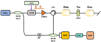
Figure 1. Experimental setup. NLL: narrow linewidth laser, OC: optical coupler, AFG: arbitrary function generator, AOM: acoustic-optic modulator, EDFA: erbium-doped fiber amplifier, Cir: optical circulator, PZT: piezoelectric transducer, PC: polarization controller, BPD: balanced photodetector, OSC: oscilloscope, DSP: digital signal processing.
Download figure:
Standard image High-resolution imageIn the experiment, a sinusoidal waveform with amplitude and frequency of 5 V and 500 Hz is first utilized to drive the PZT. In the signal demodulation, the collected signals I(t) are first converted into complex signals Ic (t) using Hilbert transform. Then the computed signal is extracted from the complex RBS signal Ic (t) with a 40 ns window function (corresponding to an effective spatial resolution of 4 m) and the corresponding spectrum is then acquired using the pulse conversion algorithm (equations (3) and (6)). Here, the chirped pulse width PW , initial frequency f0 , and bandwidth B of the chirp factor c(t) are equal to 1 µs, 70 MHz, and 260 MHz, respectively. Using the demodulation methods shown in section 2, the sensing signals (i.e. the FSs) along the whole fiber link are demodulated with fast LMS, LMS, and cross-correlation, respectively. The demodulated FS is a two-dimensional arrary and can be expressed by FS(z,t). t increases with a step of the pulse period Tp .
According to the sequence of the probe pulse, the FS distribution (along the fiber) is depicted in figure 2(a). In figure 2(a), the x-axis, y-axis, and z-axis represent the fiber distance, time, and FS, respecitvely. It can be seen that there is no abnormal signal, indicating that the spectrum demodulation is resisted to the interference fading. The applied sinusoidal vibration is clearly shown in the inset in figure 2(a). The standard deviations (SDs) of the demodulated FS using three methods are calculated to contrast their performance, as illustrated in figure 2(b). Considering that the purpose of this work is to measure dynamic strains, a detrending operation is performed for all FSs. Here, the SD at each position SD(z) is calculated as follows

Figure 2. (a) The FS distribution along the entire fiber using the fast LMS method; (b) the frequency-shift SD distribution along the entire fiber using different methods; (c) the frequency-shift SD distribution around the vibration location using different methods.
Download figure:
Standard image High-resolution imagewhere FS(z,tk ) denotes the FS of the kth measured trace (acquired by the kth probe pulse) at position z. N is the number of the collected traces which is demined by the number of the probe pulse.
As depicted in figure 2(b), the red, blue, and green lines represent the SD results calculating using fast LMS, conventional LMS (LMS), and cross-correlation (Xcorr) methods, respectively. Among these three methods, the cross-correlation (green line) method achieves the worst performance since it is susceptible to noise. The fast LMS (red line) method achieves the same performance as the LMS (blue line) method. To clearly observe the spatial resolution and vibration response, figure 2(c) shows the SDs value around the vibration position (from 7906 m to 7915 m). It can be found that the effective spatial resolution is about 4 m, which agrees well with the theoretical value of the 40 ns window function. Notice that the red line overlaps with the blue line as the proposed fast LMS algorithm is derived from the conventional LMS algorithm, and it has the same demodulation performance, only with reduced computational cost and processing time. Except for the worse performance of the cross-correlation method shown in figure 2(b), the cross-correlation method produces smaller results than LMS-based methods by comparing the results shown in figure 2(c).
In order to evaluate the demodulation performance more clearly, the frequency spectra of the RBS signals at the vibration position are extracted and illustrated in figure 3(a). The x-axis, y-axis, and z-axis in figure 3(a) represent the time, frequency, and amplitude, respectively. The shift of the spectra is related to the applied vibration. To contrast the performance of the three methods, the FS is retrieved using fast LMS, LMS, and cross-correlation methods, as depicted in figure 3(b). Here, the FS is converted into the strain according to the mathematical relationship shown in equation (5). The demodulated result using fast LMS method (red line) is completely consistent with the one demodulated by LMS method (blue line). Note that the fast LMS algorithm performs identically to the conventional LMS algorithm such that their demodulated results overlap completely (the red and blue lines). Compared with the LMS-based methods, the result demodulated with cross-correlation method is smaller since it slightly distorts the measured result. Meanwhile, the power spectral densities of these results are shown in figure 3(c). The signal-to-noise ratio (SNR) using the LMS method and the fast LMS remains the same and is equal to 41.09 dB. The cross-correlation method achieves 35.11 dB SNR, about 5.98 dB degradation in comparison with LMS-based methods.
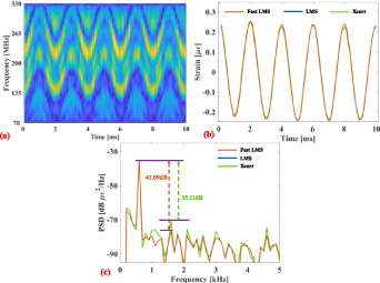
Figure 3. (a) The signal spectrum at the vibration position; (b) the retrieved time-domain waveforms using different methods, and (c) the corresponding PSDs.
Download figure:
Standard image High-resolution imageAfter that, the response of the strain with the different vibration amplitudes is tested. By tuning the voltage of PZT from 0.5 to 5 V with a step of 0.5 V, the FSs at the vibration location are retrieved using the fast LMS method, as shown in figure 4(a). Here, we add a frequency offset to each result such that all curves can be distinguished clearly. With the increment of the driving voltage, the peak-to-peak FS increases accordingly. By converting the FS to strain and fitting the peak-to-peak values of all results, the response relationship between voltage and strain is shown in figure 4(b). It can be seen that the demodulated strain is proportional to the applied voltage with a linearity of 0.9992.

Figure 4. (a) The retrieved waveforms using the fast LMS method; (b) the peak-to-peak strain with the increasing voltage.
Download figure:
Standard image High-resolution imageBesides, an amplitude-modulated vibration is also tested. The modulation frequency, carrier frequency, and modulated depth are 100 Hz, 500 Hz, and 80%, respectively. Figures 5(a) and (b) depict the frequency spectra and the retrieved time-domain waveform, respectively. The x-axis, y-axis, and z-axis in figure 5(a) represent the time, frequency, and amplitude, respectively. It can be seen that the retrieved signal is in consistent with the shift of the spectra.

Figure 5. (a) The frequency spectra of the amplitude-modulated vibration; (b) the retrieved time-domain waveform using the fast LMS method.
Download figure:
Standard image High-resolution imageAt last, the performance of the three methods is contrasted by evaluating the demodulated error and speed. Note that the demodulated error is evaluated by the variance at non-vibration positions, ![$\operatorname{var} \left( z \right) = {\left[ {SD\left( z \right)} \right]^2}$](https://content.cld.iop.org/journals/0957-0233/35/2/025101/revision2/mstad0687ieqn12.gif) . To acquire an accurate and reliable ER, the mean of the variance along the whole fiber is calculated and is expressed as
. To acquire an accurate and reliable ER, the mean of the variance along the whole fiber is calculated and is expressed as
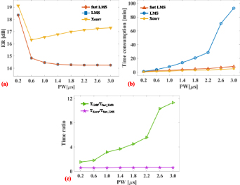
In the signal processing, the initial frequency and bandwidth are remained at 70 MHz and 260 MHz, respectively. The chirped pulse width (PW ) of the chirp factor c(t) is increased from 0.2 µs to 3 µs in a step of 0.4 µs. Figure 6(a) shows the demodulated errors using the three methods with different chirped pulse widths (PW). With the increment of chirped pulse width, the cross-correlation method achieves a minimum demodulation error at 0.6 µs chirped pulse width. For the LMS-based methods, the demodulation error gradually decreases and tends to be constant as the chirped pulse width increases. Moreover, the fast LMS method achieves the same demodulation error as the conventional LMS method (i.e. the same demodulated accuracy). However, the cross-correlation method achieves a larger measurement error (i.e. worse accuracy) since it is susceptible to random noise and easily introduces large errors, such as the results shown in figure 2(b). Compared with the cross-correlation method, the demodulation error using the LMS-based methods is reduced by ∼2.1 dB at the optimized performance (0.6 µs for the cross-correlation method and 3 µs for the LMS-based methods).
Figure 6. (a) The estimation error (ER) evolution with increasing chirped pulse width; (b) the time consumption with chirped pulse width; (c) the time consumption ratio with increasing chirped pulse width.
Download figure:
Standard image High-resolution image
Besides, the time consumption using these methods is calculated, as illustrated in figure 6(b). With the increment of the chirped pulse width, the time consumption using the LMS algorithm grows dramatically (blue line) while the processing time using fast LMS increases slowly (red line), especially for a larger chirped pulse width. That means the fast LMS operation is much faster than the conventional LMS algorithm. The cross-correlation operation has the fastest processing speed among these three methods. To contrast the time consumption of these methods more clearly, the time consumption ratios are computed and shown in figure 6(c). When the chirped pulse width increases, the time-consumption ratio between the cross-correlation and fast LMS methods remains unchanged and is approximately 0.625 (purple line), indicating that the cross-correlation method is faster than fast LMS method. Differently, the time consumption ratio between LMS and fast LMS methods increases from 1.52 times to 11.61 times as the chirped pulse width increases (green line). Especially, when a 3 µs chirped pulse width is adopted, the time-consumption using fast LMS is reduced by 11.61 times over the LMS method.
Overall, the fast LMS achieves a smaller demodulation error than the cross-correlation method (∼2.1 dB at the optimal performance), but slightly slower processing speed (∼1.6 times). Compared to the LMS algorithm, the fast LMS method has the same demodulation error but much faster processing (improvement about 12 times at the optimized performance).
4. Conclusion
A fast and accurate demodulation method is proposed for retrieving the FS using signal spectra in Φ-OTDR. By replacing the step-by-step sliding operation in conventional LMS algorithm with some simple and fast operations, the proposed fast LMS method maintains demodulation accuracy while improving the processing speed significantly. Experimental results show that the proposed method retrieves dynamic strains with a spatial resolution of 4 m over a 9 km sensing fiber. For the sensing accuracy, the proposed fast LMS method achieves the same performance as the conventional LMS method, and ∼2.1 dB improvement compared to the cross-correlation method. For the processing speed, the proposed fast LMS method achieves up to 12 times improvement than the LMS method, and 0.625 times than the cross-correlation method. Based on the above comparison, the proposed fast LMS has better demodulation performance than the two conventional methods.
Acknowledgments
This research was supported in part by National Key Research and Development Program of China under Grant 2021YFB2206303, in part by National Natural Science Foundation of China under Grants 62205275 and 61735015, in part by Fundamental Research Funds for the Central Universities under Grant 2682023CX085, in part by Sichuan Science and Technology Program under Grants 2022YFG0080 and 2022ZYD0119, and in part by Chengdu Science and Technology Program under Grant 2021-YF05-02419-GX.
Data availability statement
The data cannot be made publicly available upon publication because no suitable repository exists for hosting data in this field of study. The data that support the findings of this study are available upon reasonable request from the authors.