


Abstract
Two-dimensional (2D) self-calibration is more suitable for ultra-precision engineering than conventional calibration, as it does not require higher-precision device calibration. A grid plate is translated or rotated in various positions on a stage, and the translation and rotation can be combined into a hybrid position. Using 2D self-calibration, the stage and plate errors are separated from the overall measurement errors obtained by measuring the grid plate on the stage. During this process, random noise propagates to the separated stage errors through the self-calibration model, causing propagation of the uncertainty of the errors. Accordingly, in this study, least squares-based 2D self-calibration was investigated. An overdetermined linear equation system was established based on the relationships among the variables for self-calibration. The Guide to the Expression of Uncertainty in Measurement was used to calculate the uncertainty propagation ratio after obtaining the least squares solutions for the self-calibration model, and the uncertainty was further analyzed using the Monte Carlo method. The uncertainty propagation ratios were less than 1, indicating that the self-calibration model had a favourable noise-suppression ability. The robustness of this self-calibration approach was mathematically determined. The effects of various position schemes (with and without a hybrid position) on the uncertainty propagation ratio were examined to support the design optimisation of the self-calibration program. The experiments revealed that the use of hybrid position schemes was advantageous over not using such schemes, although the self-calibration performance was comparable under both types of schemes.
Export citation and abstract BibTeX RIS
1. Introduction
Conventional calibration assesses accuracy by comparing the measurement of an instrument with that of a reference standard, with the latter typically having a higher accuracy. For an ultra-precision instrument with an accuracy on the microscale or nanoscale, it is challenging to provide higher-quality reference standards using conventional methods [1–3]. Therefore, self-calibration (without using higher-precision measurement tools) is often applied to ultra-precision instruments to realise system error separation and compensation [4–7].
The two-dimensional (2D) self-calibration of ultra-precision instruments was first proposed by Raugh [8], aiming to resolve problems concerning calibration in electron-beam lithography. The main approaches are the Fourier transform [9, 10], rigid motion estimation [11, 12], least squares method [13–16], and optimisation [17, 18]. By measuring the coordinates of each point when a grid plate is in different positions on a stage and substituting them into a 2D self-calibration model, the system errors of the stage can be separated from the measurements. In this process, the environmental noise constituting random errors in the measurements is propagated through the self-calibration model. This affects the separated values, and results in the propagation of uncertainty. The uncertainty propagation ratio of the output to the input represents the ability of the self-calibration model to suppress noise. The evaluation of this uncertainty is helpful for determining the robustness of the method and for selecting a better self-calibration model.
In 1993, seven international organisations jointly issued the Guide to the Expression of Uncertainty in Measurement (GUM), which has since been continually revised and developed into an internationally recognised authoritative document for the evaluation of uncertainty [19–21]. Published in 2008, the Propagation of Distributions Using a Monte Carlo Method, Supplement 1 to the guide, discusses the propagation of probability distributions through a mathematical measurement model [22, 23]. The GUM method and Monte Carlo method (MCM) have been widely used in numerous fields to evaluate measurement uncertainties [24–31].
The GUM has been used to qualitatively analyse Fourier transform-based examinations of uncertainty in 2D self-calibration [32]. Owing to the complexity of the Fourier transform, the accuracy of the uncertainty obtained using the GUM is low. Moreover, the Fourier transform is difficult to express analytically, complicating the use of the GUM. Consequently, the MCM is often used for Fourier transform-based uncertainty evaluations in self-calibration [33, 34]. Least squares-based 2D self-calibration can be conducted to express the relationships between variables using linear equations, yielding results in the form of analytical solutions. Compared with other self-calibration algorithms, calculating the uncertainty propagation ratio using the least squares-based model of self-calibration is easier [35, 36]. In this study, 2D self-calibration based on the least squares method was introduced. Specifically, according to intervariable relationships, a self-calibration model of the equations was established, and the stage errors were separated using the least squares method. Next, the respective principles and processes by which the uncertainty of the 2D self-calibration was derived under the GUM and MCM were investigated. Furthermore, the uncertainty evaluations from using the GUM and MCM were compared. The connection of the uncertainty propagation ratio to the combinations of the positions (including hybrid positions) was investigated to identify a law for selecting the most-effective positions of grid plate for suppressing noise. In addition, experiments were performed to confirm that the hybrid position was advantageous for reducing the number of operational procedures, with effects similar to those of self-calibration without hybrid positions.
2. Least squares-based 2D self-calibration
In 2D self-calibration based on the least squares method, a grid plate is placed on a 2D stage as an auxiliary measuring device, and its position is changed through translation and rotation. The coordinates of each point when the plate is in different positions are determined and substituted into the self-calibration model to calculate the stage errors. The 2D self-calibration model is a linear equation system composed of measurement error functions constructed according to the intervariable relationships and properties proposed by Ye et al [9]. Because of the multiple positions examined, the equations outnumber the variables, and the self-calibration model is an overdetermined equation system. When the basic three positions, namely the initial position, a translation of a grid pitch along the X-axis or Y-axis, and a rotation of 90° around the origin, are selected, the equations satisfy the condition that the rank of the relationship matrix is equal to the number of unknowns. Moreover, they have least squares solutions, i.e. the solutions closest to the true value of the stage errors.
Figure 1 presents a flowchart of the least squares-based 2D self-calibration. It considers the three-position scheme mentioned above, i.e. the initial position, a translation of the grid distance along the positive X-axis, and a 90° counterclockwise rotation around the origin.
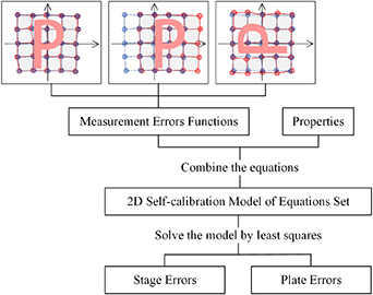
Figure 1. Flowchart of least squares-based 2D self-calibration.
Download figure:
Standard image High-resolution imageThe measurements of each marker point when the grid plate is in different positions are input into the 2D self-calibration model containing the equation set. Then, the separated stage errors can be calculated by using the least squares solutions as the outputs.
2.1. Variable definitions and relationships
In the ultra-precision field, the ideal and true values have differences, i.e. errors. The instrument used for calibration generally has multiple measurement errors. Understanding the characteristics of and relationships among the main errors is key to 2D self-calibration.
2.1.1. Variable definitions.
Three coordinate systems, namely the plate coordinate system, stage coordinate system, and machine coordinate system, are involved when the grid plate is placed on the stage and examined using a measuring machine. The marker point of a plate and its corresponding reference point in the stage coordinate system cannot be located at the exact nominal location, meaning that error vectors exist between them and the ideal points in their respective coordinate systems. Figure 2 represents the variables relative to the point at the location (m, n), namely the index of the matrix of points, the coordinates of which are (xm, yn ). The deviation between the machine and stage coordinate systems is expressed with a vector (txm, tym ) and angle θm . Similarly, the deviation between the plate and stage coordinate systems is denoted by a vector (txp, typ ) and angle θp .
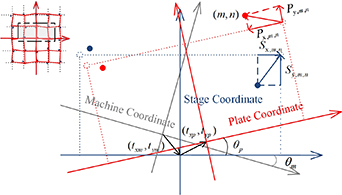
Figure 2. Variables in least squares-based 2D self-calibration.
Download figure:
Standard image High-resolution imageThe variable matrix used for 2D self-calibration can be obtained by arranging the error vectors according to the grid arrangement. Herein, the variables oriented along the X-axis and Y-axis are presented separately for clarity.
Mx, My = Measurement errors of the marker points along the X-axis and Y-axis in the machine coordinate system.
Px, Py = Errors between the marker points and ideal points along the X-axis and Y-axis in the plate coordinate system.
Sx, Sy = Errors between the ideal points and reference points along the X-axis and Y-axis in the stage coordinate system.
Ix, Iy = Coordinates of ideal points along the X-axis and Y-axis, which remain unchanged regardless of the coordinate system in which they are located.
2.1.2. Variable relationships.
To explore the relationships among variables in different coordinate systems, the variables must be transformed into one coordinate system. Specifically, Mx, My in the machine coordinate system and Px, Py in the plate coordinate system must be transformed into vectors in the stage coordinate system; this is accomplished by using the deviations among the coordinate systems.
The transformation of the coordinates of the marker points in the machine coordinate system, as examined using the measuring machine, to coordinates in the stage coordinate system is presented in equation (1). Some values can be approximated because the number of relevant variables is small
Similarly, equation (2) presents the process by which the coordinates of the marker points in the plate coordinate system are transformed into coordinates in the stage coordinate system
The coordinate values of the marker points on the grid plate in the same coordinate system should be equal. In other words, equation (1) should be equal to equation (2). The measurement errors of each marker point can be expressed as follows:
By letting θ= θm + θp, tx = txp + txm and ty = typ + tym to simplify equation (3), an equation describing the relationship between the measurements and stage errors is obtained as follows:
The reference points of the stage in the calibration area are fixed. The corresponding relationship between them and the marker points on the plate changes when the plate is transformed or rotated, resulting in changes to equation (4), mainly through the operations of Px and Py .
2.2. 2D self-calibration model of an equation set
The 2D self-calibration model is a set of equations consisting of two parts: the measurement error functions of different positions, and (based on adjustments to the coordinate systems) the properties of the variables.
2.2.1. Measurement error functions.
The centre of the grid was selected as the origin at (0, 0). For a point at (m, n), the related variables when the plate is in the initial position are related as shown in equation (4). The subscript 0 represents the initial position
When the plate is translated by a certain pitch in the positive direction along the X-axis, the reference point (m, n) on the stage corresponds to the point at (m, n− 1). The relationship between the measurements and stage errors is presented in equation (7). The subscript TX denotes the translation in the positive direction along the X-axis
Similarly, equation (8) describes the variables when the plate is rotated 90° counterclockwise, the position of which is abbreviated as R90
The translation and rotation can be combined to form a hybrid position. For example, the corresponding relationship among variables of a hybrid position R90TX, including the two aforementioned positions (translation along the X-axis and a 90° counterclockwise rotation), is expressed as shown in equation (9)
The measurement error functions for different positions are established according to the correspondence relationship between the reference points in the calibration area and the points on the plate.
2.2.2. Properties.
The coordinate systems can be adjusted using the freedom generated from the deviations among the coordinate systems. Adjustments to coordinate systems can be merged into the angle θ and vector (tx, ty ). Thus, the existence of suitable coordinate systems in which the self-calibration variables fulfil the following properties can be guaranteed [9].
The stage errors Sx, Sy undergo no translations or rotations, and have no scale differences

The plate errors Px, Py undergo no translations or rotations
The equations concerning the properties and measurement error functions of different positions constitute the 2D self-calibration model.
2.3. Least squares solutions
As previously mentioned, the number of equations in the 2D self-calibration model exceeds the number of unknowns, such that the model is an overdetermined equation set. The least squares solutions of this set are close to the true values of the variables to be determined (i.e. the stage errors Sx and Sy ). Simultaneously, approximate solutions for the plate errors Px and Py can also be obtained.
The measurements of the plate in different positions, along with the values in the equations for the properties, are the known quantity Y of an overdetermined equation set in the form AX = Y. The relationship matrix A is related to the position selection. The stage errors are included in the unknowns X, the least squares solutions for which can be expressed as X = (ATA)−1ATY. The overdetermined equation set can have a least squares solution only if |ATA|≠ 0. Under the enumeration method, the three-position scheme (the initial position, position obtained through translation, and position obtained through a 90° rotation) is a combination of the fewest positions through which these requirements are met. Here, A is the full column rank.
3. Uncertainty analysis related to 2D self-calibration
The inputs of the 2D self-calibration model were the coordinates of the marker points on the grid plate, and the outputs were the stage errors. Generally, in the process of self-calibration, measurement uncertainty is inevitable, owing to factors related to the instrument, experimenter, and operations. This uncertainty propagates to the final separated stage errors through the 2D self-calibration model. The ratio of the uncertainty of the output to the uncertainty of the input is designated as the uncertainty propagation ratio. A ratio of less than 1 demonstrates that the 2D self-calibration model can suppress environmental noise. In short, the self-calibration method proposed herein was found to be only slightly affected by external influences, and was robust.
3.1. Uncertainty propagation ratio under the GUM
The GUM is a method by which a sensitivity coefficient is calculated with regard to an evaluation of the uncertainty in the model measurements. Least squares-based 2D self-calibration involves a mathematical model containing a set of linear equations. The stage errors are analytical solutions with expressions concerning known quantities. As a result, the GUM is suitable for evaluations of uncertainty in least squares-based 2D self-calibration.
3.1.1. Uncertainty propagation ratio of least squares.
The accuracy of the estimated values X (x1, x2, ..., xt ) obtained by the least squares method is determined by the accuracy of the measured values Y and relationship matrix A. The regular expression of an overdetermined equation set AX = Y is ATAX = ATY. The measurements y1, y2, ..., yn are not correlated with each other, with the standard deviations σ1, σ2, ..., σn . The regular expression of the overdetermined equation set is expressed as follows:
Consider the example of x1. The undetermined multipliers d11, d12, ..., d1t are respectively introduced into the equations of the regular expression. The products are summed and presented as follows:
The appropriate multipliers d11, d12, ..., d1t are selected so as to satisfy the following conditions: the coefficient of x1 is 1, and the coefficients of all of the other xs are all 0. At this point, x1 can be expressed as shown in equation (17) as follows:
The coefficients of y1, y2, ..., yn in equation (17) with regard to x1 are expressed as h11, h12, ..., h1n . Thus, the uncertainty of x1 is expressed as follows:

When the measurements are equal in accuracy (that is, when σ1 = σ2, = ... = σn
= σ), owing to the conditions for the selection of the multipliers d11, d12, ..., d1t
, the uncertainty of x1 can be converted to  .
.
Similarly, the undetermined multipliers d21, d22, ..., d2t
are introduced to obtain the uncertainty of x2:  . The remaining σx
can be deduced by analogy to obtain all of the uncertainties of the unknowns. Next, the uncertainty propagation ratios of x1, x2, ..., xt
are calculated to be equal to the diagonal elements of the matrix
. The remaining σx
can be deduced by analogy to obtain all of the uncertainties of the unknowns. Next, the uncertainty propagation ratios of x1, x2, ..., xt
are calculated to be equal to the diagonal elements of the matrix  .
.
If the measurements are unequal in accuracy, P is introduced to represent the weight of the accuracy of each measurement value. The uncertainty propagation ratios of the least squares solutions are equal to the values of the diagonal elements of the matrix  .
.
The equations concerning the properties of the 2D self-calibration model are easily established through adjustments to the stage and plate coordinate systems. However, owing to the various types of noise, it is challenging to ensure that the left and right sides of the measurement error functions are perfectly equal. Thus, the weights of the property equations should considerably exceed those of the measurement error functions. The propagation of uncertainty in 2D self-calibration should be calculated under the condition that the equation set is used as a model with unequal accuracy. The weight of the property equations is generally set as at least 1 × 10⁶ times the weight of the measurement error functions in the weight matrix P. Subsequently, this weight matrix is used to calculate the uncertainty propagation ratio.
3.1.2. Uncertainty propagation ratio of each point.
Based on the derivation of the least squares solutions discussed in the previous section, the uncertainty propagation ratio of the least squares solutions for the 2D self-calibration model, i.e. the stage errors along the X-axis and Y-axis (Sx, Sy
), can be calculated according to the diagonal elements of the matrix  using the GUM.
Consider the example of a grid plate with points in an 8 × 8 arrangement. The position scheme is selected as a combination of three positions: the initial position, the position obtained by a counterclockwise rotation of 90° around the origin, and the position obtained by a translation with one pitch in the positive direction of the X-axis (i.e. a right translation). The uncertainty propagation ratio for each point as calculated using the GUM method is shown in figure 3. The uncertainty propagation ratios of all points on the plate are arranged in a 2D grid for a more impressive presentation. The results for the X-axis and Y-axis are shown separately in figures 3(a) and (b).
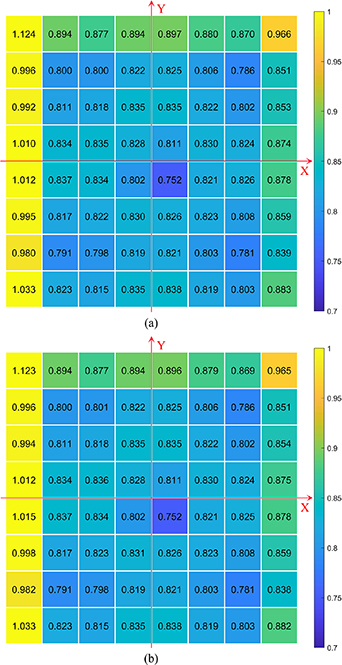
Figure 3. Uncertainty propagation ratio of each point along the (a) X-axis and the (b) Y-axis, calculated using the Guide to the Expression of Uncertainty in Measurement (GUM).
Download figure:
Standard image High-resolution imageThe number in each of the 64 boxes represents the uncertainty propagation ratio of each point. The squares are coloured to represent the uncertainty propagation ratios more vividly. The ratios corresponding to the X-axis and Y-axis directions are essentially the same, except for the values of a few points at the edges. As shown in figure 3, the uncertainty propagation ratios of points in the leftmost column approach or exceed 1, whereas those of the remaining points are less than 1. When the plate is in the position obtained by the right translation, the measurements of the points in the leftmost column are not substituted into the model for the separation of the stage errors. The uncertainties in the results calculated from the points in this column are greater than those from the other points, resulting in higher uncertainty propagation ratios.
The uncertainty propagation ratios of most points are less than 1, indicating that the uncertainty is not amplified during the self-calibration process. The uncertainties of the stage errors separated from the measurements are smaller than those of the measurements themselves. Accordingly, environmental noise is suppressed through the model, and the 2D self-calibration model exhibits favourable robustness.
3.1.3. Simulation verification.
To further evaluate the uncertainty in least squares-based 2D self-calibration, a simulation involving environmental noise was conducted. Denoted by σ, the uncertainty propagation ratio obtained by the GUM method is the normalised standard deviation of the noise. In this study, the difference between the starting values of the stage errors used to generate the measurements and the stage errors calculated by the model using the least squares method were the residuals δ, as normalised by their ratio to the standard deviation of the noise. Comparing the normalised standard deviation and residuals facilitated the determination of the influence of noise on the model results and the uncertainty analysis.
Regarding the grid plate, the same point arrangement and position scheme presented in figure 3 were used in the simulation. The stage and plate errors were both set as normally distributed random numbers with a standard deviation of 0.1 μm. These two main variables, along with other variables, were combined according to equation (4) to produce the measurements. The noise (following a Gaussian distribution with a standard deviation of 0.01 μm) was added to the simulation. The generated measurements in the three positions were substituted into the 2D self-calibration model to compute the least squares solutions of the stage errors. The computed and starting values of the stage errors Sx and Sy were compared to obtain the residuals. According to the theory related to a Gaussian distribution, approximately 95% of the values lie within two standard deviations, namely, the probability that a residual lies in the range between μ ± 2σ is approximately 95%. The mean μ here was 0. The relationship between the residuals and the interval of 0 ± 2σ is shown in figure 4.
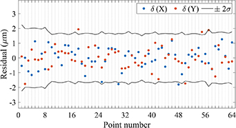
Figure 4. Relationship between theoretical uncertainties and residuals.
Download figure:
Standard image High-resolution imageThe uncertainty propagation ratios corresponding to the X-axis and Y-axis were almost equal, as shown in figure 3. Thus, the interval of ±2σ between the two black polylines was expressed using the values of the uncertainty propagation ratio on the X-axis, i.e. omitting the Y-axis. The points on the grid plate were rearranged as lines and numbered in order. In figure 4, the blue and red dots represent the residuals δ in the X-axis and Y-axis of the corresponding points, respectively. Of the 128 residuals in figure 4, there are 122 dots within the interval of 0 ± 2σ whose probability is approximately 95%, meeting the theoretical values. In the simulation, the stage errors close to true values could be separated through least squares-based 2D self-calibration in a noisy environment, confirming that noise is suppressed during 2D self-calibration (which corresponds to an uncertainty propagation ratio of <1).
3.2. Uncertainty propagation ratio under the MCM
The MCM was used to propagate the probability distribution through the model. The uncertainty was calculated according to the probability density function of the output, as obtained through the discrete sampling of the probability density function of the input following model propagation.
In 2D self-calibration based on the least squares method, the inputs are the measurements of each marker point on the grid plate, and the outputs are the stage errors calculated using the least squares method from the 2D self-calibration model involving an equation set. The relationship between variables is a linear relationship from the derivation process of the 2D self-calibration model. The uncertainties of the different variables are mutually independent without correlation. Regarding the inputs in this study, the best estimates and standard uncertainty were determined from the performance of the instrument. Thus, the probability density function was set as normally distributed. An excessive number of samples would require an excessive amount of computational time, whereas an overly small number of samples would not be representative of the whole, potentially leading to an inaccurate uncertainty assessment. Therefore, a suitable number of data points were sampled from the inputs. The samples were substituted into the model to compute the corresponding outputs. The distribution function of the output was obtained to calculate the standard uncertainty. The ratio of the uncertainty of the output stage errors to the input measurements was the uncertainty propagation ratio.
Considering the performance and computational duration of the model, a sample size of 3000 was selected to explore the uncertainty propagation ratio using the MCM. The point arrangement and position scheme of the grid plate were the same as those presented in figure 3. The representation of the uncertainty propagation ratio of each point as obtained by the MCM is the same (figure 5).
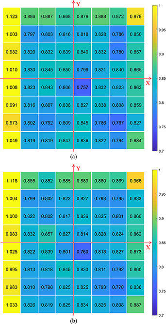
Figure 5. Uncertainty propagation ratio of each point along the (a) X-axis and the (b) Y-axis calculated using the Monte Carlo method (MCM).
Download figure:
Standard image High-resolution imageThe uncertainty propagation ratios calculated according to the MCM and presented in figure 5 are very similar to those obtained using the GUM and presented in figure 3. The root mean square of the difference between the uncertainty propagation ratios using GUM and MCM in figures 3 and 5 are 0.0103 and 0.0109 for the X-axis and Y-axis, respectively. Aside from some values in the leftmost column, most of the ratios are less than 1, indicating the favourable noise suppression capability of the model.
3.3. Joint verification of the GUM and MCM
Compared with the GUM method, which is mainly applicable to linear models, the MCM has a wider range of applications. When a model is extremely complex, the MCM forgoes the cumbersome process of derivation under the GUM method; thus, it is more convenient to use. In this study, the least squares-based 2D self-calibration had the advantage of being able to analyse the uncertainty using the GUM method relative to other self-calibrations. Both the GUM method and MCM were used simultaneously to compare the uncertainty propagation ratios of each point. The GUM was used to verify the uncertainties computed by the MCM, enabling a comprehensive evaluation of the applicability and accuracy of the uncertainty analysis method.
A comparison of the results shown in figures 3 and 5 reveals that the uncertainty propagation ratios are similar. To jointly verify the GUM and MCM, the uncertainty propagation ratios obtained under both methods are presented in one figure. The uncertainty propagation ratio equal to the diagonal elements of the matrix  is determined by the relationship matrix A, which in turn is influenced by the position of the grid plate. Figure 6 presents the uncertainty propagation ratios obtained using a grid plate with an arrangement of 64 (8 × 8) points under the GUM and MCM. The sample size under the MCM was set to 3000.

Figure 6. Uncertainty propagation ratio of each point, obtained using the GUM and MCM for different position schemes: (a) 0 + R90 + TR, (b) 0 + R90 + R90TR, (c) 0 + R90 + R180 + TR, and (d) 0 + R90 + R180 + R180TR.
Download figure:
Standard image High-resolution imageFor brevity, the positions are expressed as abbreviations. Moreover, R180 indicates a counterclockwise rotation of 180° around the origin, whereas R180TR indicates a hybrid position involving a combination of a 180° rotation and a translation of the pitch in the positive direction along the X-axis.
In the figure, the marker points are reshaped and numbered from left to right and then from top to bottom. The red and blue lines represent the uncertainty propagation ratios of each point obtained using the GUM and MCM, respectively. In all the panels, the two lines almost entirely overlap, indicating that the uncertainty propagation ratios obtained under these two methods are almost equal, regardless of the position scheme. Through the comparison, the accuracies of the uncertainty propagation ratios as calculated by the GUM method and MCM are confirmed. The two methods mutually support the premise that the ability of the model to suppress noise is demonstrated by uncertainty propagation ratios of <1 obtained through least squares-based 2D self-calibration.
The uncertainty propagation ratios were compared based on a combination of positions. A comparison of parts (a) and (b) with parts (c) and (d) of figure 6 reveals that the uncertainty propagation ratios corresponding to the four positions are considerably smaller than those corresponding to the three positions. After examining additional position schemes, we concluded that as the number of positions increases, the uncertainty propagation ratio of each point decreases. The greater the number of positions that are selected, the smaller the uncertainty propagation ratio and the stronger the suppression of noise.
The effect of hybrid positions on the uncertainty propagation ratios can be understood by comparing part (a) of figure 6 with part (b), or by comparing part (c) with part (d). The difference between the results obtained with and without the use of hybrid position schemes is not significant. The uncertainty propagation ratio of each point differs only slightly. The difference between the means of the uncertainty propagation ratios obtained with and without the use of hybrid positions is on the order of 10−8. In short, the hybrid positions do not strongly affect the theoretical uncertainty propagation ratio.
The uncertainty propagation ratios obtained using grid plates with other point arrangements were similar to those obtained using the 8 × 8 grid plate. Although the mean of the uncertainty propagation ratios increased slightly as the number of points increased, it did not exceed 1.
As mentioned, the similarity in the uncertainty propagation ratios obtained using the GUM and MCM allowed for the mutual verification of the two approaches. The patterns of variation in the uncertainty propagation ratio with respect to the different position schemes with or without the hybrid position of the grid plate, and to the number of marker points, were investigated. The smaller the uncertainty propagation ratio, the better the suppression of noise. This finding provides a theoretical basis for determining the optimal scheme for the grid plate positions.
4. Experiments
Experiments were conducted to verify the accuracy of the model-calculated uncertainty propagation ratio. A vision measuring machine (Optiv Reference 763 Dual Z) was used to measure the grid plate to enable the completion of its self-calibration. As shown in figure 7, a grid plate with evenly arranged points was placed on a device consisting of a rotation device and translation device. These two devices were controlled by a computer to transform the position of the grid plate with high precision. The vision measurement system imaged a point on the grid plate as a circle, the centre of which was the coordinate of the point. All point coordinates were measured, and the data were stored for subsequent processing under 2D self-calibration.

Figure 7. Schematic of the experimental system.
Download figure:
Standard image High-resolution imageThe pixel size of the camera of the Optiv machine is 1.70 μm/pixel when the optical magnification of the lens is 5×. The field of view is 1.3 mm × 1.0 mm, and the magnification on a 22 inch LCD is 346×. The grid plate used in this study was a quartz optical calibration plate with a production accuracy of ±0.001 mm, i.e. the range of plate errors. The pattern on the plate measured 20 mm × 20 mm and featured a 7 × 7 array of circles with diameters of 1.25 mm. The distance between the centres of the circles was 2.5 mm. The positioning accuracy and repeatability of the translation device were 50 μm and 40 μm, respectively. The positioning accuracy and repeatability of the rotation device were 0.01° and 0.005°, respectively. The vision measuring machine had a high repeatability of 0.15 μm, and was thus suitable for application in 2D self-calibration. The experiment was conducted in a stable environment with a temperature of 20 ± 1 °C and relative humidity of 50 ± 10%.
The centre of the grid plate was adjusted such that it overlapped with the centre of the rotation device. The direction of the point arrangement was adjusted such that it coincided with the translation direction of the device. The adjustments ensured that the marker points on the plate coincided with the corresponding reference points of the stage in the calibration area. The post-adjustment position was the initial position of the grid plate. The plate was rotated or translated relative to the initial position to obtain measurements at the other positions. In general, regarding simple positions, the plate must return to its initial position before it can undergo the next position change. This requirement does not apply to hybrid positions. For example, if the 0 + R90 + R90TR position scheme with a hybrid position is selected, the third position, R90TR, can be obtained by operating on position R90. Compared with the 0 + R90 + TR position scheme, the grid plate in the second position, R90, can undergo a direct translation to the hybrid position, R90TR, without having to rotate back to the initial position and then translate to obtain the position TR. Hybrid positions are more varied than simple positions, and save time by reducing the number of operations. As shown in figure 6, the uncertainty propagation ratio corresponding to the combination involving a hybrid position is clearly close to that involving only simple non-hybrid positions. The noise suppression capability is comparable under the hybrid and simple position schemes, but the operation of the hybrid position schemes was simpler. Consequently, in the determination of the position schemes of the grid plate for 2D self-calibration, hybrid position schemes are preferred.
The experimental results from the 2D self-calibration for the 0 + R90 + R90TR position scheme (figure 8) were analysed to assess the effects of hybrid positions, considering that studies on hybrid positions are relatively rare. The difference between the measurements and ideal grid is presented at 2500× magnification for clarity. The grid plates were back-translated or back-rotated to the initial position, after which the variability among the nodes in the same locations was examined. Under ideal conditions (i.e. no errors), the nodes in the same location should overlap perfectly after the plate returns to its initial position. The red, blue, and green grids in figure 8 indicate the initial position, translation of the grid distance along the positive X-axis, and 90° counterclockwise rotation around the origin returning to the same initial position. The degree of difference between the grids of different colours represents the magnitude of the errors. Because the measurements are influenced by the main factors of the plate errors Px and Py , stage errors Sx and Sy , and environmental noise before self-calibration, the nodes are spaced widely apart. After self-calibration, the stage errors Sx and Sy are successfully separated, such that the grids overlap more closely. In short, the least squares-based 2D self-calibration using hybrid positions is effective for the separation of stage errors.

Figure 8. Effect of hybrid positions on 2D self-calibration.
Download figure:
Standard image High-resolution image
The overlay, quantified as the standard deviation of the distances among the nodes in the same location, indicates the degree of variation among the grids. The overlay after self-calibration represents the effects of self-calibration. The overlay in the bottom panel of figure 8 clearly demonstrates the effects of self-calibration. A comparison of the overlay involving the hybrid position scheme 0 + R90 + R90TR with that involving the simple position scheme 0 + R90 + R90 reveals similar values; in other words, the effects of the two schemes on self-calibration are similar. The results demonstrate that operations can be simplified through the use of the hybrid position scheme, and can be transformed on the basis of the previous position without necessitating a return to the initial position and another transformation.
5. Conclusion
In this study, a 2D self-calibration model involving an equation set comprising measurement error functions corresponding to various grid plate positions was established, considering the associated properties. To expand and explore the model, a hybrid position scheme involving a combination of rotation and translation was introduced. Using the least squares method, the stage errors in the self-calibration model were separated from the measurements. The solutions were analytically expressed to facilitate an uncertainty analysis of the model using the GUM. Except for a small number of points on the edge of the plate, the uncertainty propagation ratios of the points were less than 1, demonstrating that noise suppression was achieved during the self-calibration process. A simulation verification confirmed the successful separation of the stage errors by least squares-based 2D self-calibration in a noisy environment. The MCM was employed to obtain the uncertainty propagation ratios, and was verified using the GUM method. The uncertainty propagation ratios computed under the GUM and MCM were similar for the hybrid and simple position schemes. A hybrid position was obtained through direct operation from the previous position, bypassing a return to the initial position and subsequent translation or rotation. This reduced the number of operations by one without compromising the effects of self-calibration. The experiments confirmed that 2D self-calibration performed using a hybrid position scheme enables the separation of stage errors more conveniently than that conducted using a simple position scheme.
Acknowledgment
This work was supported by the National Key Research and Development Program of China under Grant No. 2019YFF0216401.
Data availability statement
All data that support the findings of this study are included within the article (and any supplementary files).