


Abstract
Quasi-spherical cell size measurement plays an important role in medical test. The development of the lensless imaging system based lab-on-a-chip technology makes it possible to achieve the quasi-spherical cell size measurement for point-of-care test. Microfluidics based point-of-care test provide powerful platforms for biological cell detection. If you want to achieve the quasi-spherical cell size measurement in a microfluidic chip based on a lensless imaging system, the distance from the quasi-spherical cell to the imaging plane is a key parameter. In this paper, a Z-axis displacement measurement model of quasi-spherical cells based on microfluidics in the lensless imaging system is given. First, the relevant theoretical basis is introduced. Next, the Z-axis displacement measurement model is constructed based on the Fresnel diffraction at a straight edge. Then, the influence of diffraction superposition on the Z-axis displacement measurement model is explained. At last, the effectiveness and robustness of the Z-axis displacement measurement model are verified through experiments. The maximum standard deviation of the Z-axis displacement measurement is 5.86 μm.
Export citation and abstract BibTeX RIS
1. Introduction
Point-of-care testing (POCT) is defined as medical diagnostic testing at or near the point of care, that is, at the time and place of patient care [1]. The ideal POCT should be low-cost, portable, user-friendly and as simple as possible, so that even these users without professional knowledge can use it well [2]. How to achieve biological cell detection under POCT conditions has always been a research hotspot [3, 4]. Biological cell detection can be achieved through biological cell morphology measurement in measurement science [5], and it also supports the development of lab-on-a-chip (LOC) technology [6, 7]. Especially, the development of LOC technology based on lensless imaging systems makes it possible to achieve the biological cell detection for POCT [8–10].
Microfluidics has the ability to accurately control the quantity and flow rate of samples and reagents, so as to separate and detect analytes with high precision and sensitivity [11–13]. Microfluidics based POCT provide powerful platforms for biological cell detection due to many advantages such as ease-of-fabrication, low reagent use, low response time and the ability to continuously monitor and analyze.
Quasi-spherical cell size measurement plays an important role in medical test [14]. Many biological cells have a spherical or quasi-spherical shape, such as red blood cells (RBCs), white blood cells (WBCs), egg cells, cancer cells, etc. The detection of quasi-spherical cell size is of great significance in medical diagnosis. For example, circulating tumor cells (CTCs), a research hotspot in recent years, can be used to survey primary and metastatic cancer lesions through minimally-invasive peripheral blood draws, and these CTCs can be identified by the cell size [15–18].
The development of the lensless imaging system based LOC technology makes it possible to achieve the quasi-spherical cell size measurement for POCT [3, 19–24]. The conceptual structure of a typical lensless imaging system based on microfluidics is shown in figure 1. It includes three parts: a light source, a CMOS image sensor (CIS) and a microfluidic chip. The microfluidic chip containing the cells is placed directly on the CIS, and the shadows of these cells are formed on the CIS. For there is no lens between these cells and the CIS, the image of the cells cannot be truly formed on the CIS, and only the diffraction fringes of the cells are formed on the CIS [8]. How to use the lensless imaging system to obtain the information about these detected cells is a key technology and a research hotspot in recent years. The existing lensless imaging technologies for the cell detection mainly include two types: one is the lensless microscope technology based on holographic reconstruction [3, 19, 20]; the other is the cytometry technology based on diffraction fringes to obtain cell characteristics [21–25]. These two types of technologies have technical difficulties when facing the lensless imaging of cells in microfluidics.

Figure 1. Conceptual structure of a typical lensless imaging system based on microfluidics.
Download figure:
Standard image High-resolution imageGenerally, the lensless microscope technology based on holographic reconstruction has high requirements on the coherence of the light source, and needs to use a monochromatic point light source [26–30]. The cytometer technology based on diffraction fringes to acquire cell characteristics only requires a monochromatic light source [22–24]. If a monochromatic parallel light source is used to measure the cell size, one parameter can be reduced and the model can be simplified [21, 25]. Since the imaging system has no lens, the resolution of its image is very low. Therefore, a CIS with a small pixel size is needed [1]. As a carrier of biological samples, microfluidic chips have the ability to accurately control the quantity and flow rate of samples and reagents, which can greatly improve the detection capabilities of lensless imaging cell detection equipment. At the same time, due to the introduction of microfluidic chips, it will also bring some technical difficulties to lensless imaging. In a lensless imaging system, the distance ( ) from the cell to the imaging surface is a key parameter. The microchannel of the microfluidic chip has a height (h). When the cell moves in the microchannel, the cell will shift in the Z-axis direction. The distance (
 ) from the cell to the imaging plane will change, and this change is random. The uncertainty of the distance from the cell to the imaging (
 ) will seriously affect the lensless imaging systems to obtain the information of these detected cells.
In this paper, the relevant theoretical basis is introduced at first. Next, the Z-axis displacement measurement model was constructed based on the Fresnel diffraction at a straight edge. Then, we illustrate the effect of diffraction superposition on the Z-axis displacement measurement model. At last, the effectiveness and robustness of the Z-axis displacement measurement model were verified through experiments.
2. Z -axis displacement measurement model
How to obtain biological cell information through a lensless imaging system is a key technology for the practical application of a lensless imaging technology. Among various lensless imaging technologies, holographic reconstruction can obtain more information about the observed objects, and it is now the most mainstream lensless imaging technology. The reconstruction fidelity depends on the imaging resolution and the measurement accuracy and the control accuracy of the lensless imaging system, which will greatly increase the complexity of the lensless imaging system. In particular, in most holographic reconstruction technologies, the image acquisition relies on a multi-frame super-resolution algorithm, which is difficult to acquire the images of a moving object. The technique of obtaining cell characteristics based on diffraction fringes can already achieve static cell detection [21–25]. By using compatible devices to measure Z-axis displacement of cells, it can be further realized that this technique is suitable for the cell detection based on microfluidic chips.
2.1. Fresnel diffraction at a straight edge
As shown in figure 1, the CIS has a cover glass and there is a glass substrate between the cells and the imaging plane in a lensless imaging system. As the cells move in the microchannel, there is a random distance from the glass substrate which is less than the height of the microchannel. Therefore, the distance between the cell and the imaging plane is approximately hundreds of microns to millimeters. The wavelength of light source is usually several hundreds of nanometers. According to diffraction theory, the spectral line width of the diffraction pattern of a cell is larger than the diameter of the cell, so the diffraction pattern is the result of the multi-position diffraction superposition [21, 25]. Because the diffraction edge of the quasi-spherical cell is not a perfect circle, there will be different phases when different positions are superimposed. Therefore, the diffraction algorithm for perfect circular edges cannot be used. The single-edge diffraction algorithm is used to describe the quasi-spherical cell diffraction, which has greater flexibility in dealing with diffraction superposition.
Since the system as shown in figure 1 uses a parallel light source, the distance from the light source to the cells can be considered infinite. The distances from the cells to the imaging plane are approximately hundreds of microns to millimeters. The diameter of the quasi-spherical cell is generally several to more than ten microns. The light source generally uses a visible light, and the wavelength of the light is approximately several hundred nanometers. Under these conditions, the Fresnel-Kirchhoff diffraction integral can only be approximated as Fresnel diffraction, but not Fraunhofer diffraction [31].
Fresnel diffraction has been successfully applied to micro-scale measurement in various fields [32, 33]. Experiments have proved that the Fresnel diffraction at a straight edge can well describe the relationship between the position of the diffraction edge and the intensity of the diffraction fringe. If the diffraction occurs on a semi-infinite plane bounded by a sharp straight edge, the light intensity at the imaging plane can be expressed as [31]:
where  is average light intensity,
  and
and  are known as Fresnel's integrals, which can be expressed as:
and  can be expressed as:
where  is the distance to the straight edge.
  and
and  are the distance of light source and imaging plane from the cell, respectively. For a parallel light source is used in the lensless imaging system,
  .
.  can be simplified to:
2.2. Z-axis displacement measurement model
According to Huygens-Fresnel principle, every point of a wave-front may be considered as a center of a secondary disturbance which gives rise to spherical wavelets, and the wave-front at any later instant may be regarded as the envelope of these wavelets. And the secondary wavelets mutually interfere [31]. For every point of a wave-front may be considered as a center of a secondary disturbance which gives rise to spherical wavelets, adopting the straight-edge diffraction theory does not significantly change the secondary wavelets mutually interfere. The diffraction at any point on the cell edge can be regarded as the diffraction on the tangent line of the point, and the Fresnel diffraction at a straight edge can well describe the relative positional relationship between the cell edge and the diffraction fringes.
In order to describe the relationship between the diffraction pattern and the position of the quasi-spherical cell on the Z-axis, we used the position of the first bright ring of the diffraction pattern as the research object.
As shown in figure 2, this is the diffracted light intensity distribution curve, and point P is the position of the maximum light intensity point of the first bright ring. The position of P can be obtained by:

Figure 2. The curve of the diffracted light intensity (λ = 510 nm, s' = 1mm).
Download figure:
Standard image High-resolution imagewhere  is the distance to the center of the diffraction pattern. From (1), we have:
According to (2),  and
and  can be expressed as:
So,
As shown in figure 3, this curve is known as the Cornu spiral, which is useful in discussions of the general properties of the Fresnel diffraction. The point P on the curve of the Cornu spiral represent the positions of the first bright fringe of the Fresnel diffraction. At point P,  . So,
. So,

Figure 3. The Cornu spiral.
Download figure:
Standard image High-resolution imageFor a parallel light source, the distance ( ) can be expressed as:
where  is the radius of the first bright ring of the diffraction pattern. Therefore, the cell displacement in the Z-axis direction in the microchannel can be expressed as:
where  and
and  are the radius of the first bright ring of the diffraction pattern at the start and the end positions, respectively. In general, for the light path passes through a variety of different materials, such as polydimethylsiloxane (PDMS), glass, air, etc. They have different refractive indices, so the light wavelength is not a fixed value. The equivalent refractive index
  is introduced to characterize the influence of different materials on
  .
.
The relationship curve between the radius of the first bright ring of the diffraction pattern and the distance ( ) is shown in figure 4. The relationship curve shows two regularities: (1) As the radius
  increases, the slope of the relationship curve will increase, which will reduce the measurement accuracy; (2) When
  , the relationship curve has good local linearity, as shown in figures 5(a) and (b). Fortunately, for the lensless imaging of quasi-spherical cells, as the radius (
 ) increases, it means a larger diffraction pattern, which makes it easier to improve accuracy. In addition,
  is met during the Z-axis displacement measurement, so the relationship curve has good local linearity, and the measurement model can be further simplified to:

Figure 4. The relationship curve between the radius of the first bright ring of the diffraction pattern and the distance ( ).
).
Download figure:
Standard image High-resolution image
Figure 5. The relationship curve between the radius of the first bright ring of the diffraction pattern and the distance ( ) and they have good local linearity.
Download figure:
Standard image High-resolution imagewhere  can be any value between
  and
and  .
.
2.3. The effect of diffraction superposition
In a general lensless imaging system, the spectral line width of the diffraction pattern of a cell is larger than the diameter of the cell, so the diffraction pattern is the result of the multi-position diffraction superposition [21, 25].
As shown in figure 6, the radius of the quasi-spherical cell is assumed to be  , and the center of the quasi-spherical cell is defined as the coordinate origin. The light intensity of any point in the diffraction pattern is the result of the superposition of the diffracted light intensity generated by the two intersection points of the line passing through the point and the cell center and the edge of the cell. We call the point of intersection that is closer as the near-point, and the point that is farther away as the far-point. If the distance from the diffraction edge to the first bright ring of the diffraction pattern is
  , the distance between the position of the first maximum bright point of the near-point diffraction and the center of the cell is
  , and the distance between the position of the first maximum bright point of the far-point diffraction and the center of the cell is
  . Due to the superposition of light intensity, the real first maximum bright point appears between these two bright points. We define the distance from the real first maximum bright point to the cell center as
  , which is the radius of the first bright ring of the diffraction pattern.
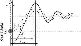
Figure 6. The diffraction intensity curve superposition of a quasi-spherical cell ( 510 nm,
  630 μm).
Download figure:
Standard image High-resolution imageThe relationship between the radius of the quasi-spherical cell and the radius of the first bright ring of the diffraction pattern under different conditions is shown in figure 7. They show that there is a similar relationship curve between the radius of the quasi-spherical cell and the radius of the first bright ring of the diffraction pattern under different conditions, and the superposition of light intensity does not change the displacement rate of the bright light ring. Suppose that the real first bright point appears in the middle of the two first bright points of the near-point diffraction and the far-point diffraction, (12) can be expressed as:
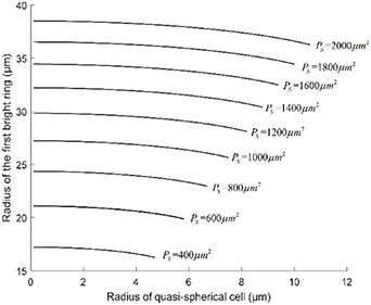
Figure 7. The relationship between the radius of the quasi-spherical cell and the radius of the first bright ring of the diffraction pattern under different conditions.
Download figure:
Standard image High-resolution imagewhere  and
and  are the radius of the first bright ring at the start and end positions of the diffraction pattern that has been considered for superposition, respectively.
  can be any value between
  and
and  .
.
3. Model validation
3.1. Super-resolution algorithms
To realize the measurement of the Z-axis displacement of the quasi-spherical cells in the microfluidic chip, it is necessary to achieve a high-precision measurement of the positions of the diffraction fringes of the quasi-spherical cells. Even using the latest CIS whose pixel size can reach 0.8 μm, the measurement accuracy cannot meet the requirements. Fortunately, there are strong regularities in the radial and circumferential directions of the diffraction pattern of the quasi-spherical cells, which can easily improve the measurement accuracy.
The dual-slope super-resolution algorithm [21] is used to improve the measurement accuracy of the diffraction fringe position. As shown in figure 8, it is the schematic diagram of the core algorithm of the dual-slope super-resolution algorithm. Pf
is the fastest rising point and Pf
is the fastest falling point. The tangent equations of the light intensity curve passing through these two points are  and
and  . The intersection of
  and
and  is point IPK, whose x-axis coordinate is considered to be the position of the maximum light intensity of the first bright ring of the diffraction pattern. Obviously, there is a certain deviation between IPK and the real maximum light intensity point IPK. Since this deviation is systematic, it will not affect this algorithm is used to calculate the Z-axis displacement measurement of a quasi-spherical cell.
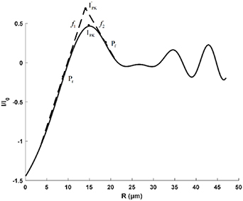
Figure 8. Dual-slope super-resolution algorithm.
Download figure:
Standard image High-resolution image3.2. Experiment system
To achieve the Z-axis displacement measurement model of quasi-spherical cells verification, we built a lensless imaging system based on microfluidics, as shown in figure 9. The system includes four parts [21, 25]:
- (1)Light source. A monochromatic parallel light source is used. As shown in figures 9(a) and (b), figure 9(a) is a dark room to avoid interference of ambient light, and figure 9(b) is a device for obtaining parallel light using a monochromatic point light source and a convex lens. The monochromatic point light source is produced by a 1 W LED with a wavelength of 590 nm and a small hole of 200 µm.
- (2)Imaging system. As shown in figure 9(d), a CIS model MT9P031 is used. The resolution is 1944 * 2592 and the pixel size is 2.2 µm.
- (3)Microfluidic chip. The microfluidic chip used in the experiment is shown in figure 9(e), with three inlets and one outlet. The inlet in the middle is used to input the sample, and the inlets on both sides are used to input the sheath fluid. Figure 9(c) shows the microfluidic chip placed on the CIS in the experiment.
- (4)Image processing system. To have better portability of the system, an embedded computer is used for image processing, as shown in figure 9(f). The embedded computer is composed of an ARM Cortex-A53 eightcore processor, 2 G DDR3 SDRAM, 32GB flash memory and 7-inch LCD screen.

Figure 9. The experiment system.
Download figure:
Standard image High-resolution image3.3. Experimental setup
As shown in figure 10, to quantitatively verify the Z-axis displacement measurement model of quasi-spherical cells model, a tilted microfluidic chip is set on the lensless imaging system. The angle between the microchannel and the imaging plane can be expressed as  . The height of the microchannel is
  . The light source uses a monochromatic parallel light source, and the light wavelength is
  .
.
3.4. Model validation
To achieve this model verification, we used a tilted microfluidic chip as shown in figure 10. We need the microspheres to produce a determinable height difference in the Z-axis direction during the movement, so the randomness of the Z-axis direction must be reduced. To prevent the random displacement of the microspheres in the Z-axis direction, we designed a microfluidic chip with a small height microchannel whose height (h) is approximately 30 μm. H1 is approximately 400 μm and L1 is approximately 19.40 mm. To increase the frame rate of the CIS, we use the region of interest (ROI) function of the CIS. The size of the ROI is 100 × 2544 pixels. The frame rate is 60 Hz. For the CIS pixel size is approximate is 2.2 µm and the lateral displacement is 2544 pixels, the length of the imaging area L2 is approximately 5596.8 µm.

Figure 10. Schematic diagram of the microfluidic system based on the lensless imaging designed to verify the proposed model.
Download figure:
Standard image High-resolution imageTo reduce the interference of other factors, the 6 μm standard size monodisperse polystyrene microspheres instead of the quasi-spherical cells are used in experiments. As shown in figure 11, they are the images formed by the microchannel of the microfluidic chip on the CIS. The image includes the trajectories of four microspheres flowing in the microchannel, and also includes the partial images of these microspheres. Figure 11 shows pictures with a starting frame, an offset of 40 frames, an offset of 70 frames, and an offset of 100 frames. Figure 12 shows the radius of the first bright ring of the diffraction pattern of four microspheres at different lateral positions. It is difficult to directly achieve model verification using the tilted microfluidic system shown in figure 8. We hope to use the tilted microfluidic system to obtain the distance  from each sample to the imaging plane as shown in figure 13(a), but the actual distance we obtain is
  as shown in figure 13(b), and
  .
.
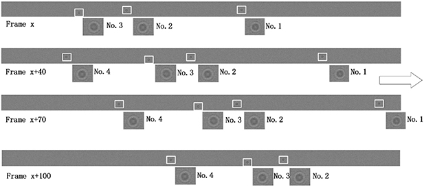
Figure 11. Microsphere imaging in a microfluidic chip.
Download figure:
Standard image High-resolution image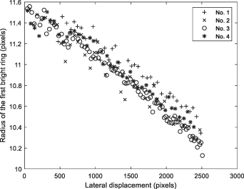
Figure 12. The relationship between the lateral displacement and the radius of the first bright ring.
Download figure:
Standard image High-resolution image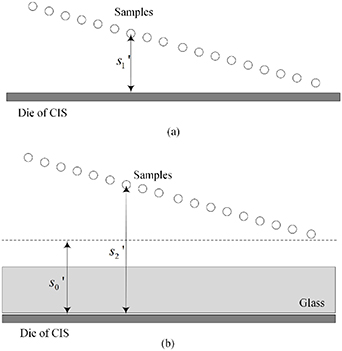
Figure 13. (a) Ideal geometric model of the experimental microfluidic system; (b) Geometric model of microfluidic system for experiment.
Download figure:
Standard image High-resolution imageThe No. 1 microsphere was used to illustrate the model verification process. According to the microfluidic system shown in figure 10, the sample position can be easily converted to Z-axis displacement. The relationship between the Z-axis displacement of the No. 1 microsphere and the first bright ring radius of the diffraction pattern obtained on the CIS is shown in figure 14. According to figure 5, since the relationship curve between the position of the first bright ring of the diffraction pattern and the distance has a very good local linearity, the position information of the first bright ring of the diffraction pattern can be obtained by the slope of the linear fitting curve.

Figure 14. The relationship between the Z-axis displacement of the No. 1 microsphere and the first bright ring radius of the diffraction pattern obtained on the CIS.
Download figure:
Standard image High-resolution imageAccording (12) or (13), we can get:
where  is the slope of the linear fitting curve. According to (10) and diffraction superposition theory, we can obtain the approximate distance from the sample to the imaging plane under ideal conditions, as shown in figure 13(a). Since we are using the slope of the linear fitting curve this time, this distance is an average distance. We can also consider this distance as the distance from the midpoint of the microchannel of the tilted microfluidic system to the imaging plane:
The distance from the sample at the midpoint of the microfluidic channel to the imaging plane is:
where  is the radius of the first bright light ring of the diffraction pattern of the sample at the midpoint of the microfluidic channel, and
  is the distance from the sample at the midpoint of the microfluidic channel to the imaging plane. So,

According figure 13,  and
and  have a good local linear relationship, and
  and
and  have a good local linear relationship, also. Assume that the first bright ring radius of the diffraction pattern of the sample at height
  on the imaging plane is
  . For it is difficult to determine the value of
  in experimental data, the average value of the radius of the first bright ring is used instead of
  , which is expressed as
  . So,
. So,

The Z-axis displacement of the sample at any position can be expressed as:
The key process data of the four samples are listed in table 1. As shown in figure 9, the thickness of the glass substrate and the cover glass are approximately 170 and 525 μm, respectively. The refractive index of them is approximately 1.5. H1 is approximately 400 μm, so the average thickness of the hollow is approximately 200 μm, and its refractive index is approximately 1. Therefore, 1.39 is taken as the weighted average refractive index. In the experiment, we use a yellow source with a wavelength of approximately 590 nm.
Table 1. The key process data in model validation.
| Index | k |
 (μm) (μm) |
 (μm) (μm) |
 (μm) (μm) |
 (μm) (μm) |
 (μm) (μm) |
|---|---|---|---|---|---|---|
| No. 1 | 39.60 | 6.30 | 24.12 | 17.82 | 176.25 | 76.52 |
| No. 2 | 39.77 | 6.33 | 23.94 | 17.61 | 188.59 | 76.95 |
| No. 3 | 37.36 | 5.95 | 23.83 | 17.88 | 187.50 | 64.54 |
| No. 4 | 41.50 | 6.60 | 24.10 | 17.50 | 193.14 | 89.42 |
The relationship between the lateral displacement and the Z-axis displacement of the four samples is shown in figure 15. It shows that the Z-axis displacement data obtained by the proposed model is in good agreement with the actual experimental settings. The deviation analysis is shown in figure 16 and table 2. Among all the Z-axis displacement data of the four samples, data with a deviation of less than 10 μm accounted for 93.87%, and the maximum standard deviation of the four samples is 5.86 μm. This shows that the proposed model is effective and has good robustness.
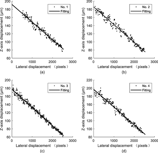
Figure 15. The relationship between the lateral displacement and the Z-axis displacement.
Download figure:
Standard image High-resolution image
Figure 16. The Z-axis displacement deviation distribution.
Download figure:
Standard image High-resolution image
Table 2. Deviation analysis.
| Index | No. 1 (μm) | No. 2 (μm) | No. 3 (μm) | No. 4 (μm) |
|---|---|---|---|---|
| Std-dev | 5.18 | 5.86 | 4.03 | 5.41 |
4. Conclusion
The Z-axis displacement measurement model can use a lensless imaging system to realize the longitudinal position measurement of the quasi-spherical cells in a microfluidic chip. If the existing lensless imaging technology is to be used in the microfluidic chip to realize cell detection, the longitudinal displacement of the cells in the microfluidic chip will bring great difficulties to these technologies. We found that the radius of the first bright ring of the quasi-spherical cell diffraction pattern and the distance from the quasi-spherical cell to the imaging plane have good local linearity. The Z-axis displacement measurement can be easily achieved by using this feature. The quantitative measurement model and method given in this paper prove to be effective and robust. The maximum standard deviation of the Z-axis displacement measurement is 5.86 μm. More importantly, the model only requires very simple experimental conditions and is very suitable for POCT.
In the microfluidic chip, this model can determine the longitudinal displacement of the cell. Combined with the existing cell detection technology based on lensless imaging, cell detection can be realized in a microfluidic chip. It can greatly improve cell throughput, improve detection efficiency and detection effectiveness. Furthermore, if the microfluidic technology can be used to make the cells controllable flip in the microfluidic chip, even the detection of the three-dimensional morphological characteristics of the cells can be realized.
Acknowledgments
This work was supported by The National Natural Science Foundation of China (Grant No. 61771388) and The National Natural Science Foundation of China (Grant No. 61471296).
Data availability statement
The data that support the findings of this study are available upon reasonable request from the authors.