


Abstract
The approach to choose the exposure sequence substantially affects the performance of the multiexposure structured light method when reconstructing the 3D shape of high dynamic range (HDR) targets. Previous researchers have conducted numerous works regarding how to select exposure time automatically, but most of them lack the consideration of the time efficiency of the 3D measurement when selecting the exposure time. In this paper, a novel approach to obtain optimal exposure for HDR targets is proposed. We developed a concept, namely, exposure style, to help us find the optimal exposure sequence. The area-weighted method is proposed as a guide to find the preliminary exposure sequence with the demanded exposure style. By uniform sampling, the preliminary exposure sequence is sampled into several alternate sequences with different lengths. By utilizing the exposure fusion method, the fused images generated by the captured images, which is under the exposures of these alternate sequences, are used to reconstruct the 3D shape of the HDR target. Then, the running time of 3D measurement and the number of generated 3D cloud points are recorded. By evaluating these two indicators comprehensively, the time efficiency of the selected exposure sequence is well-considered, and the sequence with the highest score is selected as the final optimal exposure sequence. Three HDR targets with different grayscale distributions are chosen to testify to the practicability of our method. The auto-HDR method and Zhang's method are introduced for comparison. The experimental results show that the optimal exposure sequence selected by our auto-exposure strategy performs better than other methods and the 3D shape of HDR targets can be reconstructed completely and accurately.
Export citation and abstract BibTeX RIS
1. Introduction
3D vision, as an exciting new technology, plays an irreplaceable role in automated driving, virtual reality, augmented reality, and other fields [1–3]. In the field of 3D vision, optical measurement methods are a hot topic. Structured light (SL) 3D measurement is currently the most commonly used optical measurement method due to its simple hardware configuration, high measurement accuracy, high point density, high speed, and low cost; it has found many extensive applications in industry and scientific research. For example, SL methods offer good performance in the fields of 3D face recognition, 3D reverse engineering, medical plastic surgery, industrial detection, and cultural heritage preservation [4–6].
However, classical SL techniques remain limited to ideal scenes. When the object is changed to a high dynamic range (HDR) target which has a wide surface reflectivity, such as stainless stamping, aluminum products, or other objects with a specular surface, the 3D reconstruction performances of SL techniques are severely degraded. Because the SL pattern codification strategies are mainly based on the intensity of the target surface, 18 the shiny surface has a wide range of surface reflectivity which can easily produce oversaturated and low-contrast areas in captured images. Therefore, many different techniques are proposed to improve the SL techniques to achieve the 3D reconstruction of the HDR target. Four main kinds of techniques are concluded: improving the SL pattern [7–9], changing the optical environment [10–13], utilizing the color invariance [14–16] and optimizing the captured images [17–22]. Among these methods, multi-exposure-based techniques are effective approaches in handling the specular problem. However, in most multi-exposure-based techniques, the multi-exposure sequence is usually determined empirically and is generally preferable to the reconstructed 3D results. In addition, there are many exposure combinations, and the difference between two similar exposure sequences may be small, so it is difficult to find a proper exposure sequence even when human decision is involved.
A number of experts have already conducted a series of studies on this issue. Extensive works and brilliant ideas are provided by these researchers to discover the best way to find the proper exposure sequence. In 2011, Ekstrand and Zhang developed an auto-exposure technique in which the needed exposure times can be estimated automatically based on the surface reflectivity of the measured object: a series of images of the subject at increasing exposure times are used to automatically change the image intensity without sacrificing a good fringe signal-to-noise ratio [23]. The human intervention is minimized in this method, but the single predicted exposure time is not always feasible for HDR targets.
In 2014, Feng et al presented an auto-exposure method by analyzing the surface reflectivity of the target [24]. The measured values of surface reflectivity are sub-divided into several groups based on this histogram distribution, then the optimal exposure time for each group is automatically calculated with the help of the captured intensity in this method. However, the step of dividing the surface reflectivity values into several groups is mainly conducted empirically, which makes it difficult to select the exposure time automatically.
In 2018, Rao and Da proposed an automatic multi-exposure fringe projection profilometry technique for HDR objects [25]. It is mathematically demonstrated that once the intensity modulation of a pixel exceeds a threshold, the phase quality of this pixel can be considered satisfactory. This threshold is applied to guide the computation of the required exposure times, and the intensity modulation value in the shadowing area is regarded as the threshold to terminate the computation process of the exposure time. The fringe images are then captured by automatically adjusting the exposure time of the digital camera. Nevertheless, this technique may fail to realize the 3D measurement for objects with very large surface reflectivity variations with respect to the intensity modulation value of the dark area.
In 2019, to eliminate the human intervention in adjusting the exposure time, an auto-HDR method which can automatically choose the exposure was proposed by Suming Tang and team [26]. By establishing the mathematical model of different initial groups of exposure times, the final exposure time for each group is automatically determined. Good results for the reconstruction were obtained in this work. However, the time efficiency of the final optimal exposure time is not considered in this technique.
In 2020, Zhang et al proposed a method to obtain the optimal exposure for both single and global optimal exposure determination [27]. To automatically achieve high-dynamic-range 3D shape measurement, this method needs to capture the fringe images with one exposure time. However, the numbers of the exposure sequence are not automatically decided. The time factor is not considered, and longer exposure sequences require longer processing time. This technique minimizes human invention and is implemented in the real-time 3D shape measurement system, but the time efficiency of the final optimal exposure time is still not considered.
While the above method represents an important study on how to select the optimal exposure sequence from the reflective properties of the object itself, the time efficiency of exposure time is neglected; in addition, the information of the gray histogram is not fully utilized. In this work, an auto-determined exposure sequence method based on exposure fusion is proposed for the reconstruction of the HDR object. In this method, the factors that influence the intensity on the target surface are analyzed. It is discovered that different objects have different exposure preferences. Therefore, a concept called exposure style is proposed to help us find the optimal exposure as a guide. In addition, the area-weighted method is investigated to select a proper exposure sequence with the demanded expected style. After that, different lengths of exposure sequences with the expected exposure style are obtained by uniform sampling. The time efficiency of the exposure sequence is considered by recording the running time of 3D reconstruction and the number of generated 3D cloud points as indicators, which are used to calculate the scores of the alternate exposure sequence. By ranking their scores, the optimal exposure sequences can ultimately be selected. Three specular surface objects with different exposure preferences are selected as the HDR targets in our experiments. The experiment results show that the proposed area-weighted method is useful for finding the exposure sequence with the desired exposure style, selecting the optimal exposure times, and offering effective final exposure sequence performance with respect to both time and 3D reconstruction results.
The rest of the paper is organized as follows. The introduction and related works are briefly reviewed in section 1. The proposed method is introduced in section 2. The experimental results and analyses are written in section 3. The conclusion and potential future research directions are written in section 4.
2. Proposed method
2.1. Multi-exposure based phase shift method
2.1.1. Phase shift method.
The phase shift method is utilized as the 3D reconstruction method in this work. In general, image acquisition can be divided into three steps [23]: fringe projection, fringe reflection, and fringe acquisition. Mathematically, a typical sinusoidal fringe pattern can be described as:

where A(x, y) is the average value, B(x, y) is the amplitude (or projector modulation), (x, y) represents the pixel coordinates of the projector, φ(x, y) is the phase to be determined, and δk
is the phase shift. The phase of a three-step phase-shifting algorithm with an equal phase shift of 2π/3, i.e.  , can be computed as:
The value of φ(x, y) ranges from −π to π with 2π discontinuities, which is usually called the wrapped phase. The discontinuities can be handled for a continuous phase map by adopting a phase unwrapping algorithm [6]. Once the continuous phase map is retrieved, the 3D shape of the target can be reconstructed from this phase after calibration. The same set of three equations can also generate the surface texture illuminated by the average projected and ambient light:

2.1.2. Exposure fusion.
Exposure fusion is a method that fusing a series of images into a well exposure image. Generally, this method is used in the case that the target has a HDR reflectivity surface when reconstructing its 3D shape. Three main quality measures: the contrast, the saturation, and the well-exposedness of the input images need to be calculated at first. Then all of the input images are captured by the camera. At the end, the fused result can be acquired by collapsing the input images using weighted blending. We have introduced this method in our pervious work, please see [22] for detail. With the fused images generated by exposure fusion, a set of fused images can be adopted for the calculation of phase information.
2.2. Exposure sequence and exposure style
To find the optimal exposure sequence for the HDR objects, a novel auto-exposure selection approach is proposed. Figure 1 shows the architecture of the proposed method. Our main idea for searching the optimal exposure sequence is gradually reducing the possible range by analyzing the grayscale histogram of the target. Therefore, the grayscale histogram of the HDR target is computed to calculate the probability density function. Then, the sequence with the demanded exposure style can be obtained by the area-weighted method, which will be described later. The time efficiency of exposure times is considered by recording the running time of 3D reconstruction and the number of generated 3D cloud points as indicators. By evaluating these two indicators, the sequence with the highest score is selected as the optimal exposure sequence.
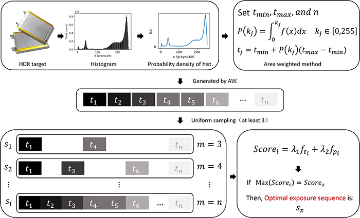
Figure 1. Architecture of the proposed method. The grayscale distribution of the HDR target histogram is quantified to calculate the probability density function of the histogram. Then, the preliminary exposure sequence with the demanded exposure style is generated by the proposed area-weighted method. By uniform sampling, the preliminary exposure sequence is sampled into several sequences with different lengths. These sequences are used to reconstruct the 3D shape of the HDR target by the multiexposure SL method, and the running time and the number of generated 3D points are recorded. By evaluating these two parameters comprehensively, the sequence with the highest score is selected as the optimal exposure sequence.
Download figure:
Standard image High-resolution imageFor a HDR object, the relationship among the pixel intensity on the image, ambient light, and projection light is as illustrated in figure 2 and can be described as:

where Ip
represents the projected light intensity on the surface of the target, β1 represents the ambient light with an intensity of β1 reflected by the object, and α represents the surface reflectivity. β2 represents the ambient light coming directly to the camera sensor with an intensity of β2. ρ represents the camera gain, and when the camera gain is set to 0 dB, ρ = 1. t represents the exposure time. Letting  , x2 = ρt, b1 = α, and
  . The equation (4) can be simplified as:

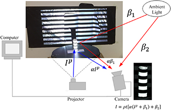
Figure 2. Relationship among the pixel intensity on the image, ambient light and projection light.
Download figure:
Standard image High-resolution imageResearchers in [26] have introduced an approach to determine the parameters in equation (5). To solve this problem, three important procedures are needed to be conducted. The first step is to set the camera gain as 0 dB, i.e. ρ = 1. The second step is to set a certain camera exposure time tc
. The last step is to project five uniform gray level patterns  onto the target surface by the projector, and to capture the images
  by the camera. Based on the captured images
  for each pixel, the parameters b1 and b2 in equation (5) can be estimated with the least square method. By this method, the relationships among exposure time t, the intensity of projection Ip
and the intensity of the image pixel can be uniquely determined. The relationship between the intensity I and exposure time t is mainly analyzed in this work. According to equation (4), the pixel intensity is linearly related to exposure time when the ambient environment is constant. However, it is difficult to find the optimal exposure sequence because there are too many combinations of exposure times. To reduce the search range, the upper and lower bounds of exposure times, as well as the length of the exposure time sequence, are limited in this work. The sequence composed of a group of exposure times from the shortest to the longest exposure time is called the exposure sequence in this work for convenience. For all exposure sequences, the length n, shortest exposure
for each pixel, the parameters b1 and b2 in equation (5) can be estimated with the least square method. By this method, the relationships among exposure time t, the intensity of projection Ip
and the intensity of the image pixel can be uniquely determined. The relationship between the intensity I and exposure time t is mainly analyzed in this work. According to equation (4), the pixel intensity is linearly related to exposure time when the ambient environment is constant. However, it is difficult to find the optimal exposure sequence because there are too many combinations of exposure times. To reduce the search range, the upper and lower bounds of exposure times, as well as the length of the exposure time sequence, are limited in this work. The sequence composed of a group of exposure times from the shortest to the longest exposure time is called the exposure sequence in this work for convenience. For all exposure sequences, the length n, shortest exposure  , and longest exposure
  are the basic elements.
  is defined as the exposure time for which details can be observed clearly in a specular area, and nothing can be seen with reduced exposure time.
  is defined as the exposure time in which the shape of the target is clear in the captured image and there is no under-exposure area on the surface of the target. The length of the preliminary exposure sequence n is usually between 5 and 13. This value will not affect the length of the final optimal exposure sequence. With these constraints, the problem can be transferred to finding an optimal exposure sequence with known
  ,
,  and n.
Three types of objects with different surface grayscale distributions are listed in figure 3. For the first object, the black metal nut as shown in figure 3(a), its grayscale histogram exhibits separate concentrations in the range of 20–80 and the range of 150–180. The second object, the soft package lithium battery as shown in figure 3(c), has a brighter surface than the nut, and its grayscale histogram is mainly concentrated in the range of 170–255. The third object, the stainless stamping as shown in figure 3(e), has the brightest surface, and its grayscale histogram is mainly concentrated in the range of 250–255. We find that when the exposure time tends to be distributed under some specific distribution, these exposure sequences perform well. To describe these unique exposure sequences, the combination of different exposure times with unique distribution is called 'exposure style'. Exposure style is proposed to help us find the optimal exposure sequence as a guide. Once the shortest and the longest exposure time are fixed, the exposure sequence with different exposure style shows its exposure style. It is not difficult to ascertain that the optimal exposure sequence of the three objects must have a complementary exposure style with their surface grayscale distributions in order to help display more surface detail.
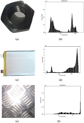
Figure 3. Images of three targets and their grayscale histograms: these images show how significantly the distributions of their grayscale values vary. (a) Image of the black metal nut. (b) The grayscale histogram of the black metal nut. (c) Image of the soft packing lithium battery. (d) The grayscale histogram of the soft packing lithium battery. (e) Image of the stainless stamping plate. (f) The grayscale histogram of the stainless stamping plate.
Download figure:
Standard image High-resolution imageTo make it more normative, a uniformly distributed exposure sequence is defined as a standard exposure sequence that has an even exposure style. Here we introduce the exposure value concept to explain this.
Under the same ISO value and iris aperture, the luminous flux will be doubled when the exposure time increases two-fold. It means that the luminous flux positively correlates with exposure time:

where F refers to the iris aperture, T refers to exposure time, and EV refers to exposure value. When the value of T increases by  times, EV decreases linearly. Then, we obtain an exposure sequence as follows:

where i refers to the number of exposure times in the sequence. Ti
refers to the ith time in the sequence. Larger order numbers correspond to longer exposure times. We define that the exposure sequence that makes EVs vary linearly is the standard exposure sequence. The exposure times in this sequence can be regarded as evenly distributed between  and
and  .
.
According to this definition, the exposure sequence computed by equation (7) is uniformly distributed. The exposure sequence has an even exposure style. This sequence is a geometric series. The reason for this definition is that the dynamic range of the HDR object's luminance is large, and it is necessary to increase the exposure sequence proportionally in order to capture the details of the HDR object's surface better.
According to equation (4), we know that I is linearly related to the exposure time t. Therefore, the subscript of the selected time represents the light intensity level corresponding to that time.
Supposing that the environment is constant, the footnotes at each time in the standard exposure time series can represent the corresponding intensity level.
With the standard exposure sequence generated by equation (7), the exposure sequences with different exposure styles can be obtained by selecting exposure times from this standard exposure sequence. For example, supposing we have generated an exposure sequence with length of 8 and that the sequence is  , t8; the exposure sequence with dark style can be represented by selecting
  , t8; the exposure sequence with even style can be represented by selecting
  , t8; the bright style can be represented by selecting
  , t8.
, t8.
The experiment results support our speculation that the optimal exposure sequence for a target shows a complementary character link with the surface grayscale distribution. To illustrate the validity of this claim, a set of comparison experiments are designed with a soft packing lithium battery as an example. The related experimentation is presented in section 3.
By analyzing the exposure style which the target prefers, the searching field of the optimal exposure sequence is narrowed. The exposure style shows a distribution of exposure times for the optimal exposure sequence. Therefore, finding the exposure sequence with a demanded exposure style is important for automatically seeking the optimal exposure sequence.
2.3. Area-weighted method
To find the exposure sequence with the demanded exposure style of a given target automatically, an area-weighted method is proposed in this work.
In the area-weighted method, the grayscale histogram of the HDR target is divided into n equally divided regions, and the ratio  between the area of each region and the area of all regions is recorded. For each node
  , the final ratio ri
can be calculated by
, the final ratio ri
can be calculated by  . These ratios can also be obtained from the probability accumulation function by integral as follows:
where f(x) is the probability density function of the image (i.e. the percentage of points with a given grayscale value). With these ratios, the exposure sequence with demanded exposure style can be computed as:

where kj ∈[0, 255], j = 1, 2, ..., n for an 8-bit camera image.
Figure 4 shows that the exposure sequence selected by the area-weighted method can generate an exposure sequence with the expected exposure style. As illustrated in figure 4, the area-weighted method finds the preference of the HDR target well and offers a reference for exposure sequence selection.

Figure 4. Area weight curve of a dark surface target and a bright surface target generated by the proposed area-weighted method. The values of the percentage tend to cluster in high-value regions for the dark surface target so that the exposure sequence with a bright exposure style can be generated. The values of the percentage tend to cluster in low-value regions for the light surface target so that the exposure sequence with a dark exposure style can be generated.
Download figure:
Standard image High-resolution image2.4. Auto-exposure strategy
The proposed auto-exposure strategy can be conducted in four steps as following:
Step 1: The camera gain is set as 0 dB, i.e. ρ = 1, then the aperture of the camera lens is adjusted to a proper position where there are as few saturated areas as possible in the captured image while projecting a uniform pattern with the gray value of 250. The shortest exposure time  , the longest exposure time
  and the length of the preliminary exposure sequence
  can be obtained from the definitions in the previous section.
Step 2: After setting  ,
,  , and n, the uniform exposure sequence can be generated by equation (7). Then, finding a proper exposure time in the uniform exposure sequence ensures that there are no saturated areas in the captured image. The probability density function f(x) is then calculated by normalizing the grayscale histogram of the captured image. The preliminary exposure sequence is generated by equation (9).
For example, supposing that the target is the black metal nut as mentioned in figure 3, we set  ms,
ms,  ms and n = 6. As illustrated in figure 5, the histogram is divided into six parts separately indexed as k = 0, 51, 102, 153, 204, and 255. According to equation (8), we obtain a sequence with percentage P(kj
) calculated as 0.0%, 32.0%, 55.0%, 58.0%, 97.0%, 99%, and 100%. As calculated by equation (9), the preliminary exposure sequence is 2, 10.96, 17.4, 18.24, 29.16, and 29.72 ms.
ms and n = 6. As illustrated in figure 5, the histogram is divided into six parts separately indexed as k = 0, 51, 102, 153, 204, and 255. According to equation (8), we obtain a sequence with percentage P(kj
) calculated as 0.0%, 32.0%, 55.0%, 58.0%, 97.0%, 99%, and 100%. As calculated by equation (9), the preliminary exposure sequence is 2, 10.96, 17.4, 18.24, 29.16, and 29.72 ms.

Figure 5. The grayscale histogram and the area weight curve of the black metal nut.
Download figure:
Standard image High-resolution image
Step 3: In order to find the optimal exposure sequence with the desired exposure style. The preliminary exposure sequence is recorded as M, where  . The lengths of the alternate exposure sequences obtained from uniform sampling were taken as n = 3, 4, ... , m, respectively. They are recorded as
  .
.
Step 4: The running time of 3D measurement timej and the number of the 3D cloud points pj are recorded when the alternate exposure sequence Mj is used to reconstruct the 3D shape of the target. At this step, we find the final optimal exposure sequence from the alternate exposure sequence by evaluating timej and pj , as described below:
We set  ,
, 
 ,
,  , and γ
 0.8. The time index
  can be described as
  . The point index can be described as
  . fnorm
represents the normalization function:
. fnorm
represents the normalization function:
The score of the alternate exposure sequence Mj can be calculated as follows:

Generally, the running time index and cloud point index are treated with the same importance. Therefore, we set λ1, λ2 to 0.5.
By ranking the scores, the optimal exposure sequence with the highest score can be found.
3. Experiments
We built a SLS to evaluate our proposed method. The SLS consists of one LCD (XGIMI, 500-899ANSI) with a resolution of 1080 × 1920 pixels as the projector and a camera (Da-Heng, USB3.0, interface, 14 fps) with a resolution of 3840 × 2748 pixels.
3.1. Verification of the exposure style and area-weighted method
As mentioned in section 2, the message we seek to convey is that the optimal exposure sequence for a target must have a complementary exposure style with the surface grayscale distribution. An object with a dark appearance (overall darkness in the grayscale histogram distribution) will not choose an exposure sequence with the same dark style but will choose an exposure sequence with a light style that is complementary to it; similarly, an object with a uniform grayscale distribution will prefer a style with an even exposure time distribution, and an object with a bright grayscale distribution will prefer a style with a dark exposure time distribution.
The soft packing lithium battery and cylindrical lithium battery are selected as the targets. Four kinds of exposure styles are designed for comparison: dark, slightly dark, slightly light, and light, as shown in table 1. The result for the cylindrical lithium battery is shown in table 3. In this experiment, the  ,
,  and n are set as 2 ms, 128 ms and 13, respectively.
Table 1. Four exposure sequences with different exposure styles.
| Exposure style | Exposure sequence |
|---|---|
| Dark |

|
| Slightly dark |

|
| Slightly light |

|
| Light |

|
Table 2. Scores for soft package lithium battery.
| Exposure style | Time (s) | Points | Scores |
|---|---|---|---|
| Dark | 3898.4 | 2379 220 | 0.2408 |
| Slightly dark | 4051.1 | 2493 625 | 0.2493 |
| Slightly light | 3952.0 | 2541 466 | 0.2579 |
| Light | 3969.1 | 2495 804 | 0.2521 |
Note: The bold number means the highest score.
Table 3. Scores for cylindrical lithium battery.
| Exposure style | Time (s) | Points | Scores |
|---|---|---|---|
| Dark | 2222.3 | 407 944 | 0.1777 |
| Slightly dark | 2180.0 | 482 028 | 0.3268 |
| Slightly light | 2143.7 | 482 731 | 0.3303 |
| Light | 2158.3 | 399 748 | 0.1651 |
Note: The bold number means the highest score.
Results in tables 2 and 3 show that for the slightly dark style objects (soft packing battery and cylindrical lithium battery), the slightly light style exposure sequence is more suitable than the others.
From the experimental results, it can be seen that the soft pack battery and the cylindrical lithium battery, both belonging to the slightly dark style, are more suitable for the selection of exposure time in the slightly bright style. The experiment shows that the different exposure styles of the exposure sequence greatly influence the 3D reconstruction results of the same measurement object and that the suitable exposure style can enable a better measurement effect of the selected exposure sequences.
However, finding an exposure sequence with a demanded exposure style requires significant time if we adopt the method mentioned above. Therefore, the area weighted method is used instead of manual selection. To show the value of this method, we design an experiment for comparison.
The area-weighted method is used to select the exposure sequence automatically. The results in tables 4 and 5 show that the exposure sequence generated by area-weighted method can be close to the demanded exposure sequence and have the same exposure style as the expected exposure style and that the proposed area-weighted method can serve as a guide to find the target's exposure preference, i.e. the exposure sequence with the demanded exposure style.
Table 4. Comparison result for the exposure sequences generated by manual and area-weighted methods for the soft packing lithium battery.
| Generated method | Exposure sequence |
|---|---|

| |
| Manually designed | 2.0, 3.0, 23.0, 32.0, 45.0, 64.0, 90.0, 128.0 |
| Area-weighted method | 2.0, 5.2, 17.6, 26.9, 37.8, 47.5, 52.2, 128.0 |
Table 5. Comparison result for the exposure sequences generated by manual and area-weighted methods for the cylindrical lithium battery.
| Generated method | Exposure sequence |
|---|---|

| |
| Manually designed | 2.0, 3.0, 23.0, 32.0, 45.0, 64.0, 90.0, 128.0 |
| Area-weighted method | 2.0, 9.1, 17.3, 25.0, 37.8, 55.5, 77.6, 128.0 |
3.2. Auto-exposure strategy experiments
We verify our auto-exposure method by testing on the soft packing lithium battery, which is a classical HDR target. To reflect the advantages of our method, two representative methods: the auto-HDR [26] method and Zhang [27] method are selected for comparison.
The setup procedure of our method includes setting the camera gain as 0 dB, i.e. ρ = 1, then adjusting the aperture of the camera lens to a proper position where there are as few saturated areas in the captured image as possible.  and
and  can be obtained by the criterion introduced in section 2. For the soft packing lithium battery,
  and
and  are obtained as 2 ms and 128 ms, respectively. The length of the preliminary exposure sequence n is set as 13. With the help of the area-weighted method, the ratio of each exposure time in the demanded sequence is calculated as shown in figure 6, the preliminary exposure sequence M can be obtained by equation (9), and the sequence is shown in table 6.

Figure 6. Grayscale histogram and area weight figure for the soft packing lithium battery.
Download figure:
Standard image High-resolution imageTable 6. Preliminary exposure sequence for the soft packing lithium battery.
| Exposures (ms) | Percentages (%) |
|---|---|
| t1 = 2.0 | 0.02 |
| t2 = 4.6 | 2.07 |
| t3 = 12.4 | 8.27 |
| t4 = 16.4 | 11.46 |
| t5 = 18.9 | 13.39 |
| t6 = 24.0 | 17.44 |
| t7 = 31.4 | 23.32 |
| t8 = 38.9 | 29.26 |
| t9 = 48.6 | 36.95 |
| t10 = 61.2 | 46.94 |
| t11 = 74.1 | 57.25 |
| t12 = 86.5 | 67.08 |
| t13 = 128.0 | 100.00 |
Then, the alternate exposure sequence Mj
, j = 1, 2, ..., 13 with different length is selected by uniform sampling of the preliminary exposure sequence M. The results are shown in table 7. For each alternate sequence Mj
, the running time index  of 3D reconstruction and the points index
  are recorded in table 7. The related parameters (Q, R, p0,
  and the point index
  are calculated in table 7. Scores of the alternate exposure sequence are calculated by equation (11), and the result is shown in table 8.
Table 7. Alternate exposure sequence for the soft packing lithium battery.
| n | Sequences | Exposure sequences |
|---|---|---|
| 3 | s1 |

|
| 4 | s2 |

|
| 5 | s3 |

|
| 6 | s4 |
|
| 7 | s5 |
|
| 8 | s6 |

|
| 10 | s7 |

|
| 12 | s8 |

|
Table 8. Recorded results and scores of the soft packing lithium battery.
| n | Sequences | Time (s) | Points |

|

| Scores |
|---|---|---|---|---|---|---|
| 3 | s1 | 2007.4 | 1461 099 | 0.195 | 0.009 | 0.102 |
| 4 | s2 | 2324.3 | 1750 953 | 0.168 | 0.053 | 0.111 |
| 5 | s3 | 2740.3 | 2306 022 | 0.143 | 0.137 | 0.140 |
| 6 | s4 | 3029.8 | 2286 404 | 0.129 | 0.134 | 0.132 |
| 7 | s5 | 3633.7 | 2511 699 | 0.108 | 0.168 | 0.138 |
| 8 | s6 | 3952.0 | 2541 466 | 0.099 | 0.173 | 0.136 |
| 10 | s7 | 4525.6 | 2483 807 | 0.087 | 0.164 | 0.125 |
| 12 | s8 | 5511.1 | 2458 261 | 0.071 | 0.160 | 0.116 |
Note: The bold number means the highest score.
The results in table 8 show that exposure sequence s3 in table 7 achieved the highest score of 0.140 in the comprehensive evaluation, which means that s3 is the optimal exposure sequence after considering both running time and cloud points. The final exposure sequence for the soft pack lithium battery calculated by our method is 2.0, 16.4, 31.4, 61.2, and 128.0 ms as shown in table 9. The final exposure sequence of the auto-HDR method is 3.5, 6.4, 11.5, 20.7, 37.2, and 67.0 ms. The final exposure sequence of Zhang's method is 2.0, 2.3, 3.2, 6.0, 21.3, and 265.0 ms. The 3D reconstruction results of the three methods are illustrated in figure 7.
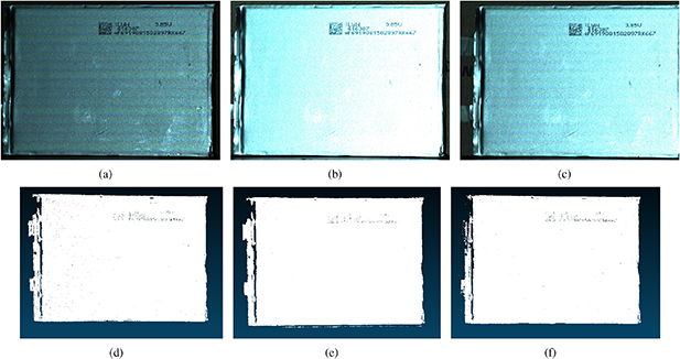
Figure 7. Measurement result of the soft packing lithium battery. (a) Image fused by the exposure sequence generated by auto-HDR method. (b) Image fused by the exposure sequence generated by Zhang's method. (c) Image fused by the optimal exposure sequence generated by our method. (d) 3D result using exposure sequence in (a). (e) 3D result using exposure sequence in (b). (f) 3D result using optimal exposure sequence.
Download figure:
Standard image High-resolution imageTable 9. Final optimal exposure sequence for the soft packing lithium battery.
| Exposures (ms) | Percentages (%) |
|---|---|
| t1 = 2.0 | 0.02 |
| t4 = 16.4 | 11.46 |
| t7 = 31.4 | 23.32 |
| t10 = 61.2 | 46.94 |
| t13 = 128.0 | 100.00 |
The experiment results in table 10 show that our method obtains the highest score of 0.365 when comparing with other methods. To evaluate the precision of the reconstructed results, the objects sprayed with white powder are reconstructed as the ground truth. By comparing the experiment results with the standard model, the average absolute error of different methods are calculated. The average absolute error can be calculated by equation (12). The comparison of the three methods is shown in tables 10, 15 and 20.
Table 10. 3D reconstruction results of the soft packing lithium battery with auto-HDR, Zhang and our method.
| Method | Accuracy (mm) | Time (s) | Points | Scores |
|---|---|---|---|---|
| Auto-HDR [26] | 0.1528 | 2959.7 | 1557 221 | 0.304 |
| Zhang [27] | 0.1606 | 3105.6 | 1626 674 | 0.331 |
| Our method | 0.1408 | 2209.9 | 1578 501 | 0.365 |
where the X represents the 3D coordinates of the measured cloud points and Y represents the 3D coordinates of the standard model. acc is the average absolute error. n is the valid number of cloud points.
The 3D reconstruction result illustrated in figure 7 shows that the 3D shape of the HDR target can be effectively recovered by the proposed auto-exposure method. As illustrated in table 7, the number of 3D points grows slowly when the length of the exposure sequence is larger than 5. At the meanwhile, the processing time keeps on increasing. It means that the advantage of this sequence in generating the 3D cloud points is being replaced by the disadvantage in spending time. By comprehensive evaluation, the sequence with good performance in both time efficiency and 3D reconstruction is selected.
To testify the practicability of our method, another two HDR objects with different grayscale distributions are chosen for the experiments. The first one is a black metal bracket as shown in figure 8. The second one is shown in figure 9: a stainless stamping plate that has a strong reflection property. Similar to the experiment mentioned above, by analyzing the grayscale distribution of these two targets, the preliminary exposure sequence can be calculated with the area-weighted method. Notice that the camera sensitivity is set to 0 dB, the aperture of the camera lens is fixed at the same value as in the first experiment, and the initial parameters are set as  ms,
ms,  ms, n = 8 and
  ms,
ms,  ms, n = 8, respectively. The area weights figures are shown in figures 10 and 11. All of the exposure times and alternate exposure sequences can then be calculated by our auto-exposure strategy, as listed in tables 11, 12, 16 and 17. The recorded results and scores are listed in tables 13 and 18. The final exposure sequences are listed in tables 14 and 19.
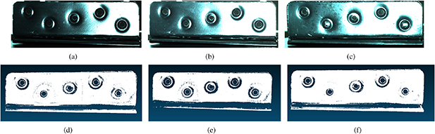
Figure 8. Measurement results of the black metal bracket. (a) Image fused by the exposure sequence generated by auto-HDR method. (b) Image fused by the exposure sequence generated by Zhang's method. (c) Image fused by the optimal exposure sequence generated by our method. (d) 3D result using exposure sequence in (a). (e) 3D result using exposure sequence in (b). (f) 3D result using optimal exposure sequence.
Download figure:
Standard image High-resolution image
Figure 9. Measurement results of the stainless stamping plate. (a) Image fused by the exposure sequence generated by auto-HDR method. (b) Image fused by the exposure sequence generated by Zhang's method. (c) Image fused by the optimal exposure sequence generated by our method. (d) 3D result using exposure sequence in (a). (e) 3D result using exposure sequence in (b). (f) 3D result using optimal exposure sequence.
Download figure:
Standard image High-resolution image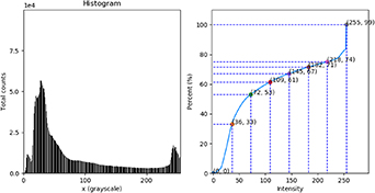
Figure 10. Grayscale histogram and area weight figure for black metal bracket.
Download figure:
Standard image High-resolution image
Figure 11. Grayscale histogram and area weight figure for stainless stamping plate.
Download figure:
Standard image High-resolution image
Table 11. Preliminary exposure sequence of for the black metal bracket.
| Exposures (ms) | Percentages (%) |
|---|---|
| t1 = 3.0 | 0.02 |
| t2 = 68.4 | 37.79 |
| t3 = 107.8 | 56.74 |
| t4 = 124.1 | 64.83 |
| t5 = 135.3 | 70.08 |
| t6 = 143.8 | 73.82 |
| t7 = 150.7 | 76.69 |
| t8 = 200.0 | 100.00 |
Table 12. Alternate exposure sequence for the black metal bracket.
| n | Sequences | Exposure sequences |
|---|---|---|
| 3 | s1 |

|
| 4 | s2 |

|
| 5 | s3 |

|
| 6 | s4 |

|
| 7 | s5 |
|
| 8 | s6 |

|
Table 13. Recorded results and scores for the black metal bracket.
| n | Sequences | Time (s) | Points |

|

| Scores |
|---|---|---|---|---|---|---|
| 3 | s1 | 2075.796 | 1308 549 | 0.245 | 0.092 | 0.168 |
| 4 | s2 | 2471.472 | 1365 256 | 0.205 | 0.112 | 0.159 |
| 5 | s3 | 2867.369 | 1626 068 | 0.177 | 0.204 | 0.190 |
| 6 | s4 | 3405.297 | 1618 628 | 0.149 | 0.201 | 0.175 |
| 7 | s5 | 4236.619 | 1606 001 | 0.120 | 0.197 | 0.158 |
| 8 | s6 | 4871.71 | 1601 511 | 0.104 | 0.195 | 0.150 |
Note: The bold number means the highest score.
Table 14. Final optimal exposure sequence for the black metal bracket.
| Exposures (ms) | Percentages (%) |
|---|---|
| t1 = 3.0 | 0.02 |
| t2 = 68.4 | 37.79 |
| t4 = 124.1 | 64.83 |
| t6 = 143.8 | 73.82 |
| t8 = 200.0 | 100.00 |
Table 15. 3D reconstruction results of the black metal bracket with auto-HDR, Zhang and our method.
| Method | Accuracy (mm) | Time (s) | Points | Scores |
|---|---|---|---|---|
| Auto-HDR [26] | 0.1420 | 4277.8 | 2175 984 | 0.302 |
| Zhang [27] | 0.1389 | 4202.3 | 2162 376 | 0.300 |
| Our | 0.1237 | 3858.4 | 2426 365 | 0.398 |
Table 16. Preliminary exposure sequence for the stainless stamping plate.
| Exposures (ms) | Percentages (%) |
|---|---|
| t1 = 2.0 | 0.01 |
| t2 = 2.0 | 0.02 |
| t3 = 2.4 | 0.79 |
| t4 = 7.5 | 11.50 |
| t5 = 18.0 | 33.20 |
| t6 = 27.5 | 53.10 |
| t7 = 35.0 | 68.80 |
| t8 = 50.0 | 100.00 |
Table 17. Alternate exposure sequence for the stainless stamping plate.
| n | Sequences | Exposure sequences |
|---|---|---|
| 3 | s1 |

|
| 4 | s2 |

|
| 5 | s3 |

|
| 6 | s4 |

|
| 7 | s5 |
|
Table 18. Recorded results and scores for the stainless stamping plate.
| n | Sequences | Time (s) | Points |

|

| Scores |
|---|---|---|---|---|---|---|
| 3 | s1 | 2394.237 | 2254 508 | 0.270 | 0.187 | 0.232 |
| 4 | s2 | 2994.207 | 2270 467 | 0.214 | 0.193 | 0.207 |
| 5 | s3 | 3388.97 | 2324 720 | 0.176 | 0.216 | 0.206 |
| 6 | s4 | 3919.202 | 2296 099 | 0.159 | 0.204 | 0.187 |
| 7 | s5 | 4910.569 | 2289 613 | 0.130 | 0.201 | 0.168 |
Note: The bold number means the highest score.
Table 19. Final optimal exposure sequence for the stainless stamping plate.
| Exposures (ms) | Percentages (%) |
|---|---|
| t1 = 2.0 | 0.01 |
| t5 = 18.0 | 33.2 |
| t8 = 50.0 | 100.00 |
Table 20. 3D reconstruction results of the stainless stamping plate with auto-HDR, Zhang and our method.
| Method | Accuracy (mm) | Time (s) | Points | Scores |
|---|---|---|---|---|
| Auto-HDR [26] | 0.1719 | 3164.1 | 1020 889 | 0.393 |
| Zhang [27] | 0.0991 | 2273.9 | 428 186 | 0.211 |
| Our | 0.1203 | 2081.0 | 853 050 | 0.395 |
With the computed exposure time, the related fringe images for these two targets can be captured automatically. The fused images for these two objects by three methods are shown in figures 8(a)–(c) and 9(a)–(c), respectively. The experiment results in tables 10, 15 and 20 show that our proposed method acquired a higher score than the other two methods. Especially in table 15, the exposure sequence selected by our method takes the least time and generates the most 3D cloud points. In tables 10 and 20, the number of the 3D clouds points generated by the exposure sequence selected by our method decreases about 3% and 16% to the most one. However, the running time of our selected exposure sequence decreases about 25% and 34% when comparing with the longest one. It shows the advantage of our method that the time efficiency and the quality of the 3D reconstruction are considered at the same time. From these images, it can be found that the reconstructed 3D shapes for these two HDR targets are accurate and complete. These experimental results demonstrate that our proposed auto-exposure technique has potential practicability in industrial applications.
4. Conclusion
The way we choose the exposure sequence severely affects the performance of the multi-exposure-based SL method, especially when a human decision intervenes. Therefore, automatically determining the exposure sequence is vitally important for the reconstruction of the HDR target. In this work, a novel approach to obtain optimal exposure for HDR targets is proposed. In this approach, the exposure preference of the target is analyzed by recording the grayscale histogram of the target's image. The area-weighted method is proposed to calculate the preliminary exposure sequence with demanded exposure style. By uniform sampling, alternate exposure sequences with different lengths can be obtained from the preliminary exposure sequence. After utilizing the exposure fusion procedure, the running time of 3D measurement and the number of generated 3D cloud points for each alternate exposure sequence can be respectively recorded. The exposure sequence with the highest scores is selected as the optimal exposure sequence when considering these two indicators. Experiments show that our SLS can accurately reconstruct the 3D shape of the HDR target through several exposures by applying our method. The contribution of the proposed technique is that the time efficiency of the exposure sequence is considered when comparing with other related works. The proposed method can provide better three-dimensional reconstruction and has the highest time efficiency. In addition, the area-weighted method is originally proposed to help us find the exposure sequence with the demanded exposure style. The method also shares some limitations: in the final step, to find the best exposure sequence, the multiple exposure sequence must be tested, which is time-consuming. In the next work, we will focus on how to simplify the process of our proposed method without losing stability.
Acknowledgments
This work was supported in part by the National Natural Science Foundation of China under Grant Nos. U1801263 and U1701262, and by the Intelligent Manufacturing Comprehensive Standardization and New Model Application Project of the Ministry of Industry and Information Technology of the People's Republic of China.
Data availability statement
No new data were created or analysed in this study.