


Abstract
The comprehensive influence of the amplitude and frequency of the modulated magnetic field and the magnitude of the bias magnetic field on the performance of an atomic magnetometer have been investigated. Under different magnetic fields, the combined action of the spin precession signal caused by a high-amplitude magnetic field and the influence of magnetic field on relaxation makes the time domain output signal and the amplitude of the first to fourth harmonics show different characteristics, which cannot be explained by the classical analytical calculation solution. By considering the influence of the magnetic field on the transverse relaxation, a more complete model is constructed to explain the phenomenon with a numerical solution, and the overall fit is 93.26%. Based on the single beam and magnetic field modulation scheme, a compact magnetometer is constructed for verification, with a volume of 56.7 cm3 and a sensitivity of 30 fT/Hz1/2.
Export citation and abstract BibTeX RIS
1. Introduction
Since the realization of the spin-exchange relaxation-free (SERF) regime in 2002 [1], atomic magnetometers can realize ultra-high sensitivity magnetic measurements. In 2010, a SERF-based magnetometer was shown to achieve the highest sensitivity for a measurement with an extremely weak magnetic field [2], and further development is envisaged. By taking full advantage of the integrated micro-optical [3], the magnetometer noise suppression [4], and the microfabricated rubidium vapour cell [5], the magnetic field sensing area is reduced to less than 10 cm2 [6]. Atomic magnetometer arrays show promise for application in the biomedical field, including magnetocardiography [7, 8] and magnetoencephalography [9, 10].
Atomic magnetometers have a variety of configurations based on the optical path, such as the pump–probe beam geometry [11], the two-color pump–probe scheme [12], and nearly parallel pump and probe beams [13]. In order to reduce the volume of the magnetometer, the probe beam is omitted, and the configuration of a single pump beam superimposed with transverse magnetic field modulation is adopted [14]. The transmitted intensity manifests a zero-field resonance, which is a Lorentzian function of the magnetic field components transverse to the laser beam [15]. The influence of the small modulated magnetic field on the magnetometer can be solved analytically by the Bloch equation [16]. The first harmonic component manifests an absolute dispersion function of the bias magnetic field [17]. Using Bessel functions and first-order linear differential equations, a strict formula of the transmitted intensity can be solved [18]. However, the effect of the magnetic field on the relaxation cannot be ignored as it increases. As a result, the output response of the magnetometer is not only the superposition of sinusoidal signals, but also the higher harmonics and spin precession signals [19, 20]. These phenomena cannot be explained by previous analytical solutions. Using numerical software for solving differential equations and substituting the calculation parameters into the initial formula, the approximate solution can be obtained. In this paper, the calculated value is in good agreement with the experimental value, which verifies the correctness of the comprehensive influence of the magnetic field on the magnetometer.
2. Theory
In the atomic magnetometer, the change in polarizability can be described by the Bloch equation:
 is the electron spin polarization vector.
  is the electronic Larmor precession frequency including the direction vector, which is equal to the gyromagnetic ratio of the bare electron γ, considering the slowing-down factor q times the vector magnetic field. q is the nuclear slowing-down factor that accounts for angular momentum storage in the alkali metal nucleus. When the spin of the Rb atom (nuclear spin I = 5/2) is highly polarized, the nuclear slowing-down factor is given by
  . T is the combined effect of relaxation decoherence and pumped positive excitation on the atomic polarization. Under weak pumping beam intensity, the relaxation in the longitudinal lifetime T1 can be derived from the linewidth obtained by scanning the magnetic field perpendicular to the direction of the pump beam. It is dominated by wall collisions
  and spin-destruction collisions
  with other alkali atoms, buffer gas atoms, and quenching gas molecules. A further change in the laser intensity is used to obtain a pumping rate under the corresponding laser intensity. The transverse relaxation T2 additionally includes the dephasing of the magnetic field to the non-quantization axis [21]. The ratio of spin-exchange broadening
  to the magnetic field is related to the effective value of the magnetic field [22].
  is the optical pumping rate for an unpolarized atom, which is related to the absorption cross-section and photon flux.
  is the spin angular momentum of the pumping photons in the propagation direction of the pump. This vector has a magnitude equal to the degree of polarization, and the circularly polarized laser contains one unit of angular momentum. Pumping in the direction of the circularly polarized laser changes the polarizability, reaching transient equilibrium under the combined action of the Larmor precession of atomic spins and the coherence depolarization. The intensity of the pumping beam passing through the cell is proportional to the polarizability [23]. By applying a high-frequency modulated magnetic field along the sensitivity axis so that the resonant atom operates in a near-SERF state, this reduces the attenuation of the signal-to-noise ratio caused by the linewidth increase [17].
The direction of the laser is defined as coinciding with the Z axis. After shielding, the magnetic field around the magnetometer is reduced to pT level and with the assumption that ΩY
= 0 and ΩZ
= 0. The magnetic field applied to the X axis is  . Thus, equation (1) can be expanded as follows:

As the magnetic field increases, the atom undergoes a transition from a SERF state to a non-SERF state. Since  , it is difficult to directly merge
  and
and  into a complex form and use the Bessel functions to convert the trigonometric term in the exponent into a Fourier series [24]. Therefore, numerical solutions are used here instead of analytical solutions to obtain the specific values of
  under different magnetic fields.
K1 to K8 are the simplified parameters used for fitting the calculated and experimental data points. K1, K2, and K3 are the proportional coefficients of the bias field amplitude, the modulated field amplitude, and the modulated field frequency, respectively.  is the coefficient representing the electron relaxation influence on the polarization, including the cell temperature, heating frequency, and cell parameters (and can be refined into cell shape, alkali metal content, atmosphere ratio, and air pressure).
  is the coefficient describing the effect of the pumping rate on the polarization, including laser intensity and frequency. When the magnetometer works stably, the corresponding parameters remain unchanged. Thus, K4 and K5 become constants and it is not necessary to determine them during the curve fitting process. When the laser penetrates the atom cell, the photodiode converts the laser intensity fluctuations into a current signal, which then passes through a transimpedance amplifier, a filter (to eliminate the interference of high-frequency heating), and a demodulator to form the final voltage amplitude curve. The signal conversion and signal loss through the above instrument sequence are combined into the scale factor K9. The numerical solution
  is then multiplied by K9 to compare the overall graph similarity. It should be noted that K5 is normalized to 1. The pumping rate influence on the lifetime is merged into K4 and its influence on the signal strength is merged into K9. As the modulation frequency increases, the influence of the modulated magnetic field on the relaxation attenuates, and the two show an exponential relationship described by the K6 coefficient [25]. K7 and K8 are the second- and first-order coefficients of the magnetic field on the relaxation, respectively.
3. Experimental set-up
A compact magnetometer was constructed and used to verify the correctness of the calculation results. The auxiliary equipment was similar to the general platform optical path [26], but many stabilization mechanisms were removed in order to reduce its volume [27]. The single-beam magnetometer cannot measure the magnetic field in the direction of the pumping beam, so the axial and tangential magnetic fields can be measured simultaneously through two reflections of the optical path instead of the straight-through optical path [28], as shown in figure 1(a). The compact magnetometer, as shown in figure 1(b), contained a cubic cell with an internal side length of 3 mm and a wall thickness of 0.5 mm. The alkali metal 87Rb and nitrogen at 1.5 atm pressure were used. The laser frequency was 795 nm, and the power of the cell-incident was 1 mW. The cell temperature was set to 413 K, while the heating frequency was 300 kHz [29]. Inside three-layer magnetic shields, a calibrated magnetic field of 100 pT rms@20.5 Hz was applied to calculate the normalized power spectral density (PSD) of the output signal (red curve), as shown in figure 1(c). The noise floor was ∼ 30 fT/Hz1/2 (blue line). However the low-frequency range was slightly worse, and the bandwidth could be extended to 120 Hz.

Figure 1. (a) Magnetometer system block diagram. PMF: polarization maintaining fiber; F: fiber port; L: collimating lens; R: reflector; PD: photodetector; TA: transimpedance amplifier; LIA: lock-in amplifier; DAQ: data acquisition. (b) Picture of the magnetometer probe with a size of 3.15 cm × 1.8 cm × 10 cm. (c) The normalized PSD of the output signal (red curve) is used to characterize the sensitivity of the magnetometer. The noise floor was ∼ 30 fT/Hz1/2 (blue line).
Download figure:
Standard image High-resolution image4. Result and discussion
4.1. Function of magnetic field on relaxation
The relationship between the magnetic field and the relaxation can be obtained by the scanning linewidth method, while other influences remain unchanged. With respect to the pumping beam in the Z direction, the influence of the X and Y directions magnetic fields is symmetrical. In the experiment, different bias magnetic fields are applied on the Y axis, and a scanning magnetic field is applied on the X axis to obtain the corresponding Lorentz curve. The fitting error bar was marked with 95% confidence bounds. The half width at half maximum (HWHM) of each curve represents the magnetic field relaxation under the bias magnetic field. As shown in the blue curve in figure 2, the relaxation manifests a quadratic function of the magnetic field, when the bias magnetic field is small. With a fitting function of HWHM = 0.006By2 + 0.12By + 25.23, the fitting is 99.92%. As the bias magnetic field increases, the relationship between HWHM and the magnetic field becomes a linear function, as shown in the green curve in figure 2. With a fitting function of HWHM = 0.82By + 4.15, the fitting is 99.99%. In order to facilitate the fitting calculation, the relationship between relaxation and the magnetic field is simplified as a quadratic function, as shown in equation (5).
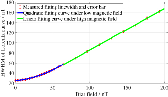
Figure 2. The relationship between the bias magnetic field in the Y direction and the HWHM of the Lorentz curve obtained by scanning the magnetic field in the X direction. The red markings indicate the measurement of HWHM with an error bar under different bias magnetic fields. The blue and green curves represent the fitting curve of the relationship between the bias magnetic field and the HWHM.
Download figure:
Standard image High-resolution image4.2. Time domain graph of output response amplitude under different modulation frequencies, modulation amplitudes, and bias magnetic fields
The simplified analytical solution shows that when the bias magnetic field is zero, the response of the magnetometer to the small modulated magnetic field is the second harmonic [24]. The bias magnetic field can be obtained by demodulating the first harmonic, which is the basic working principle of the modulated magnetometer. When the amplitude of the modulated magnetic field is large, its effect on the magnetometer is similar to a pulsed magnetic field. The spin precession signal caused by a large modulation amplitude magnetic field cannot be ignored, resulting in the time domain waveform no longer being a superposition of standard sine waves. Therefore, in one modulation period, the response of the magnetometer shows two transient response signals, which contain high-order even harmonics. The magnetic field is set at the optimum sensitivity of the magnetometer at the center: modulation amplitude 200 nT, modulation frequency 800 Hz. A comparison of the applied magnetic field parameters and corresponding characteristics is shown in table 1. The time domain response of the magnetometer to different magnetic fields is shown in figure 3.
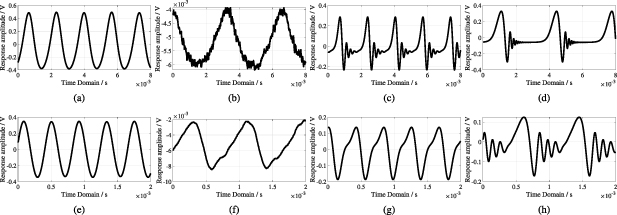
Figure 3. The response of the magnetometer in the time domain under different bias magnetic fields and modulated magnetic field amplitudes and frequencies.
Download figure:
Standard image High-resolution imageTable 1. Comparison of parameter settings and corresponding characteristics from figure 3.
| Number | Modulation amplitude | Modulation frequency | Bias amplitude | Characteristic | Comparison |
|---|---|---|---|---|---|
| a | 127.8 nT | 300 Hz | 0 nT | 2nd harmonic | Higher amplitude |
| b | 766.8 nT | 1st harmonic (close to noise) | |||
| c | 766.8 nT | 0 nT | Even harmonics | ||
| d | 766.8 nT | Even and odd harmonics | |||
| e | 127.8 nT | 1200 Hz | 0 nT | 2nd harmonic | Lower amplitude |
| f | 766.8 nT | 1st harmonic (close to noise) | |||
| g | 766.8 nT | 0 nT | Even harmonics | ||
| h | 766.8 nT | Even and odd harmonics |
4.3. Comparison of calculation and experimental graph of different order harmonics under different magnetic fields
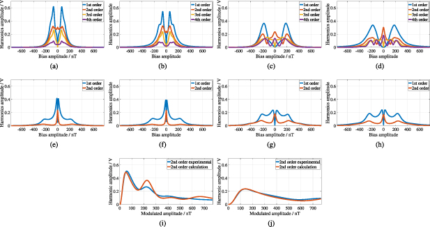
Under different magnetic fields, a lock-in amplifier is used to demodulate the time domain signal under different order harmonics to obtain the corresponding harmonic amplitude. The harmonic curve is scanned with bias magnitude or modulation amplitude as the independent variable (1000 points per curve). The scanning frequency of the experimental curve is very low, about 5 mHz, so the modulation component introduced by the scanning magnetic field can be ignored. The magnetic field parameter settings and the corresponding fit are shown in table 2. The harmonic amplitude curve is shown in figure 4. To maximize the overall fit, we optimize eight fitting parameters (K5 is normalized to 1) and substitute them into equations (2)–(5) for numerical calculation. The coefficient of determination is used to characterize the fit. The fitting parameters  were set to
  , and K9 = 1323. The overall fitting accuracy of 14 000 experimental points and corresponding calculated points in 14 curves is 93.26%. The degree of fit does not reach 100%, which may have secondary reasons such as the magnetic field gradient and uneven heating. In the simplified formula [17], the increase of the unidirectional bias field causes the first harmonic to increase first and then decrease. However, in figures 4(a)–(g), the spin precession signal introduced by a larger bias magnetic field makes the descending process of the first harmonic no longer monotonous, which is consistent with the time domain shown in figure 3. The other high-order harmonics also show a similar law of changes.
Figure 4. Graphs (a)–(h) show the amplitude of the first- to fourth-order harmonics as a function of the bias magnetic field. The amplitude of higher harmonics at high frequencies tends to zero, which is not marked. Graphs (i, j) show the amplitude of the second-order harmonic as a function of the modulation amplitude. All the calculation graphs use the same set of parameters. The overall fitting accuracy of 14 000 experimental points and corresponding calculated points in 14 curves is 93.26%.
Download figure:
Standard image High-resolution image
Table 2. Parameter settings and corresponding fit in figure 4.
| Number | Type | Modulation amplitude | Modulation frequency | Bias amplitude | Harmonic order | Line fit | Overall fit |
|---|---|---|---|---|---|---|---|
| a | Experimental | 127.8 nT | 300 Hz | Independent variable | 1st (blue) | — | |
| 2nd (red) | |||||||
| 3rd (yellow) | |||||||
| 4th (purple) | |||||||
| b | Calculation | Basic amplitude × 1 | Basic frequency × 1 | 1st (blue) | 94.31% | 95.54% | |
| 2nd (red) | 97.01% | ||||||
| 3rd (yellow) | 98.92% | ||||||
| 4th (purple) | 94.06% | ||||||
| c | Experimental | 255.6 nT | 300 Hz | 1st (blue) | — | ||
| 2nd (red) | |||||||
| 3rd (yellow) | |||||||
| 4th (purple) | |||||||
| d | Calculation | Basic amplitude × 2 | Basic frequency × 1 | 1st (blue) | 91.67% | 89.67% | |
| 2nd (red) | 89.76% | ||||||
| 3rd (yellow) | 91.71% | ||||||
| 4th (purple) | 74.32% | ||||||
| e | Experimental | 127.8 nT | 1200 Hz | 1st (blue) | — | ||
| 2nd (red) | |||||||
| f | Calculation | Basic amplitude × 1 | Basic frequency × 4 | 1st (blue) | 97.91% | 98.04% | |
| 2nd (red) | 99.40% | ||||||
| g | Experimental | 255.6 nT | 1200 Hz | 1st (blue) | — | ||
| 2nd (red) | |||||||
| h | Calculation | Basic amplitude × 2 | Basic frequency × 4 | 1st (blue) | 92.85% | 93.34% | |
| 2nd (red) | 95.84% | ||||||
| i | Experimental | Independent variable | 300 Hz | 0nT | 2nd (blue) | — | |
| Calculation | Basic frequency × 1 | 0 | 2nd (red) | 89.48% | 89.48% | ||
| j | Experimental | 1200 Hz | 0nT | 2nd (blue) | — | ||
| Calculation | Basic frequency × 4 | 0 | 2nd (red) | 94.49% | 94.49% | ||
5. Conclusion
Focusing on the magnetic field corresponding to the optimal sensitivity of the magnetometer, the modulation frequency, modulation amplitude, and bias amplitude are appropriately extended, and the comprehensive influence of the magnetic field on an atomic magnetometer is studied. The time domain graphs show the superposition of multiple harmonics of spin precession signals instead of standard sine waves. The harmonic graphs show the coexistence of multiple harmonics, not just low-order harmonics. None of these phenomena can be explained by traditional analytical solutions. By considering the influence of the magnetic field on the transverse relaxation, numerical solutions are used to fit a large number of experimental graphs, and a good degree of fit is obtained. Having a more comprehensive mechanism for the magnetic field in the magnetometer is essential to the improvement of sensitivity.
Acknowledgments
This work was supported by the National Natural Science Foundation of China (NSFC) 61627806, the National Key R&D Program of China 2018YFB2002405, and the Beijing Natural Science Foundation (4191002).